Article

Improved U-Net Remote Sensing Classification Algorithm Fusing Attention and Multiscale Features

1
School of Automation, Guangxi University of Science and Technology, Liuzhou 545006, China
2
National Satellite Meteorological Center, China Meteorological Administration, Beijing 100081, China
*
Author to whom correspondence should be addressed.
Remote Sens. 2022, 14(15), 3591; https://doi.org/10.3390/rs14153591
Submission received: 9 June 2022 / Revised: 23 July 2022 / Accepted: 24 July 2022 / Published: 27 July 2022
(This article belongs to the Special Issue Remote Sensing for Mapping Farmland and Agricultural Infrastructure)

Abstract

:
The selection and representation of classification features in remote sensing image play crucial roles in image classification accuracy. To effectively improve the features classification accuracy, an improved U-Net remote sensing classification algorithm fusing attention and multiscale features is proposed in this paper, called spatial attention-atrous spatial pyramid pooling U-Net (SA-UNet). This framework connects atrous spatial pyramid pooling (ASPP) with the convolutional units of the encoder of the original U-Net in the form of residuals. The ASPP module expands the receptive field, integrates multiscale features in the network, and enhances the ability to express shallow features. Through the fusion residual module, shallow and deep features are deeply fused, and the characteristics of shallow and deep features are further used. The spatial attention mechanism is used to combine spatial with semantic information so that the decoder can recover more spatial information. In this study, the crop distribution in central Guangxi province was analyzed, and experiments were conducted based on Landsat 8 multispectral remote sensing images. The experimental results showed that the improved algorithm increases the classification accuracy, with the accuracy increasing from 93.33% to 96.25%, The segmentation accuracy of sugarcane, rice, and other land increased from 96.42%, 63.37%, and 88.43% to 98.01%, 83.21%, and 95.71%, respectively. The agricultural planting area results obtained by the proposed algorithm can be used as input data for regional ecological models, which is conducive to the development of accurate and real-time crop growth change models.

Graphical Abstract

1. Introduction

Remote sensing technology plays an important role in agricultural monitoring, geological survey, military survey, and target detection [1,2,3,4]. As a use of remote sensing technology, land cover classification is a hot and challenging research topic. Accurate land cover classification is important for agricultural production and grain yield assessment, urban planning and construction, and ecological change monitoring [5,6,7]. Researchers have proposed multiple classifiers to classify land cover using remote sensing images [8], and the classification methods based on optical satellite images can be broadly grouped into spectral-based and spectral–spatial classification methods [9]. The spectrum-based classification methods use the spectral values obtained from remote sensing images as features, and statistical clustering or machine learning classification algorithms, including support vector machines (SVMs) [10], maximum likelihood [11], and random forest [12], to classify pixels. The spectral–spatial-based classification methods combine their own spectral values and construct corresponding auxiliary information from the image neighborhood space as feature vectors to achieve pixel-by-pixel classification of remote sensing images [13].
Although the above classifiers can accurately classify land cover, they still need to be improved for precision agriculture classification. Thus, with the development of deep learning, classification methods based on deep learning have been widely used for land cover classification, such as convolutional neural networks (CNNs) [14,15,16,17,18,19], improved Transformer [20,21], etc. U-Net [22], as an earlier CNN, was initially applied for segmenting medical images because U-Net only needs a small batch of data to produce accurate segmentation results. U-Net has also been applied for land cover classification tasks by many researchers, who have proposed many improved U-Net network structures to improve the semantic segmentation performance [23,24]. The U-Net model consists of an encoder and a decoder. The encoder extracts high-level features through a step-by-step downsampling operation. The decoder gradually upsamples the high-level features, and combines the skip connection to restore the feature map to the original size. U-Net loses large amounts of detailed information during downsampling; therefore, adding ASPP to U-Net helps to retain this detailed information while increasing the perceptual field [19]. Zhang et al. [14] added an ASPP module to the underlying U-Net, enabling the feature maps to be extracted with multiscale contextual information and reducing the confusion between different types of adjacent pixels. To overcome the problem of poor image contour recovery in the decoder process of U-Net, a conditional random field (CRF) was added to U-Net for post-processing [17]. CRF processing can reduce mixing between similar ground object types. The Res-UNet proposed by Cao et al. [15] is an organic combination between ResNet [25] and U-Net [22], where the residual unit of ResNet replaces the convolutional layer of U-Net so that shallow features more easily propagate to deep layers, improving the distinction between features with small differences in spectral signatures.Yan et al. used U-Net to extract features at different levels, input them into SVM classification, and performed a majority voting game on the classification results of features at different levels, fully considering the effects of shallow, mid-level, and deep-level features [16]. Biserka Petrovska et al. [26] used a combination of CNN and SVM with linear and radial basis function (RBF) kernels (RBF SVM), which extracts features by the fine-tuned CNN to put into the RBF SVM for classification. Biserka Petrovska et al. [27] used a variety of mainstream CNNs to extract features from remote sensing images, fused the features extracted by different CNNs, and put them into SVM for classification. The U-Net + SVM approach requires the features extracted from U-Net to be input to SVM training, and SVM training is a time-consuming process. U-Net++, proposed by Chen et al. [28] uses dense skip connections and subnetwork nesting to improve U-Net, but not all skip connections are beneficial for segmentation tasks, so some skip connections negatively affect the results [29]. Remote sensing images contain rich spectral and spatial information, so selecting feature information favors classification is essential [30]. The attention mechanism excels in natural language processing (NLP) and computer vision tasks. The attention mechanism can highlight features with strong representation ability and suppress irrelevant features [31,32,33]. Therefore, the attention mechanism has been introduced into remote sensing image classification by many researchers. The attention mechanisms commonly used in remote sensing images include the channel attention, spatial attention, and self-attention mechanisms [34]. Channel attention focuses on what is input, whereas spatial attention focuses on the location of the information, and spatial attention is complementary to channel attention. Channel attention uses global average pooling and global max pooling to obtain the relationship between feature channels to generate channel attention maps, and spatial attention uses average pooling and max pooling along the channel axis to obtain spatial feature attention maps [32]. Zhu et al. [35] enhanced the bands with strong characterization ability and suppressed irrelevant bands by introducing a spectral attention module that assigns different weights to the bands, improving the spatial attention mechanism that allows the network to assign neighboring pixel weights, and finally combining it with the residual unit to achieve high accuracy on the Indian Pines, University of Pavia, Kennedy (http://www.ehu.eus/ccwintco/index.php?title=Hyperspectral_Remote_Sensing_Scenes accessed on 1 January 2021). Different from directly embedding the attention module in the residual unit, Attention-UNet [18] reduces the redundant features transmitted by the skip connections by adding attention gates to the U-Net skip connections, and highlights the salient features in specific local regions. High-resolution remote sensing images have certain features. Self-attention was originally used for NLP tasks. Due to the excellent performance of Transformer [34], Alexey et al. [36] proposed Vision Transformer (ViT) using the encoder part of Transformer. Although ViT performs well on large datasets such as imageNet, its memory consumption is large, so ViT has high hardware requirements. To improve efficiency, Chen et al. [37] proposed TransUNet, which uses the image blocks from the feature map of CNN for the input sequence of ViT, and then combines it with U-Net. The decoder upsamples the output features of ViT and then combines it with the CNN feature map of the same size to recover the spatial information, which effectively improves the semantic information of the image. Because the Swin Transformer [38], having powerful global modeling capability, has shown superior performance on several large visual datasets, some researchers have combined the Swin Transformer with U-Net to achieve semantic segmentation [20,21,39]. The Swin Transformer used by ST-UNet [20] was paralleled with CNN to improve the accuracy of small-scale target segmentation by combining the global features of the Swin Transformer with the local features of CNN through an aggregation module.
The algorithms described above, having different improved optimization approaches for different classification tasks, provided the reference ideas for the study described in this paper. To further improve the classification accuracy of remote sensing images, the deepening of the network was experimentally found to lead to the reduction in spatial resolution and the divergence in spatial information. Therefore, in this paper, an improved U-Net remote sensing classification algorithm that integrates attention and multiscale features is proposed. First, the algorithm uses dilated convolutions of different scales to expand the receptive field so that the network effectively integrates multiscale features and enhances shallow features. Second, through the fusion residual module, the shallow and deep features are deeply fused, and the characteristics of shallow and deep features are effectively used. Third, to integrate more spatial information into the upsampling feature maps, a spatial attention module (SAM) is used to fuse the feature maps obtained from skip connections with the upsampling feature maps to enhance the combination of spatial and semantic information.
In this paper, U-Net is combined with ASPP and SAM to improve and optimize it for land cover classification from Landsat 8 remote sensing images. The main contributions include (1) exploring the effect of different hierarchical features of U-Net on the ground cover classification of 30 m resolution Landsat 8 images; (2) introducing the ASPP module to perform residual connections with the original U-Net, which not only increases the fusion of multiscale features but also enhanced the expression of shallow information; (3) introducing SAM to obtain the spatial weight matrix for the feature maps with richer spatial information, so that the spatial weight matrix acts on the corresponding semantic feature maps to obtain the feature maps combining spatial and semantic information; and (4) conducting dynamic change analysis of land use in the study area, focusing on the dynamic change in the crop planting area.
The rest of the paper is structured as follows: Section 2 introduces the experimental data, the data processing methods, and the effects of different level features on Landsat 8 image ground cover classification. The proposed improved U-Net model is also described. Section 3 outlines the experimental results in detail. Section 4 provides a discussion based on the experimental results, and conclusions are drawn in Section 5.

2. Materials and Methods

2.1. Study Area Overview

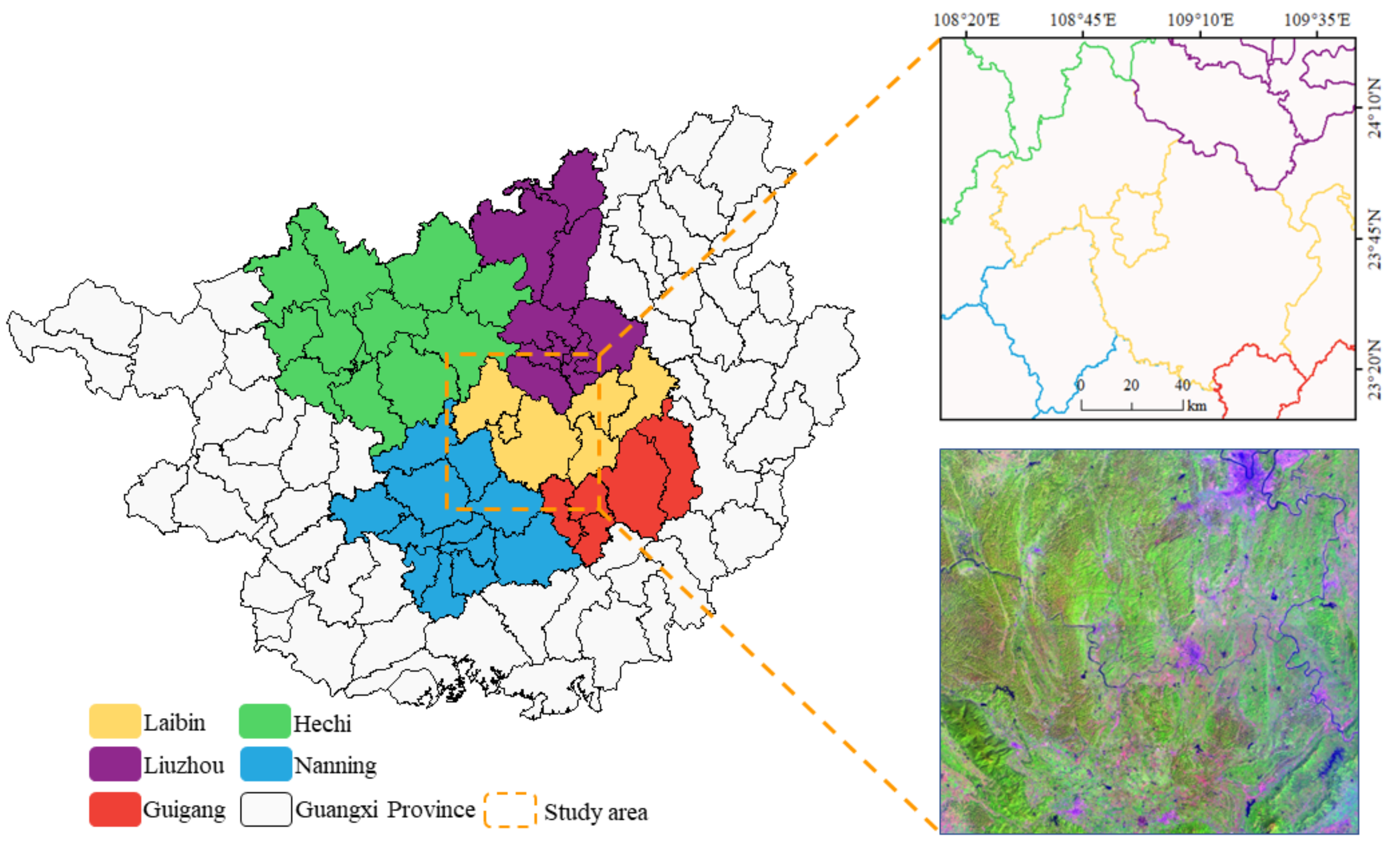
Guangxi Province is located in South China; Guangxi has a subtropical monsoon climate with a tropical monsoon season and warm climate, abundant rainfall and sunshine. Guangxi has some of the most abundant precipitation in China, so the province is suitable for fruit and crop cultivation, including citrus, mango, banana, lychee, sugarcane, rice, and so on. The landscape is generally composed of six categories: mountains, hills, terraces, plains, rocky hills, and water surface. The area selected for this study is located in the central part of Guangxi Zhuang Autonomous Region, mainly including Xingbin District, Heshan District and Xincheng County of Laibin City, Liujiang District of Liuzhou City, and Shanglin County of Nanning City. The study area is located 108°19′9″E–109°47′26″E and 23°3′29″N–24°23′54″N (Figure 1). Its unique climatic and geographical factors make sugarcane and rice the main crops in Guangxi, where sugarcane and rice have two seasons per year. Sugarcane and spring sowing are from January to March and harvest occurs from May to August; autumn sowing is from August to September and harvest is in December. The first rice season ranges from sowing in April to harvesting in July, and the second season is July to October. The area under sugarcane accounts for about 60% of the total sugarcane cultivation area in China. The sugarcane planting area in the study area is mostly continuous, exceeding 64% of the total agricultural land. As such, accurately and effectively determining the planting area of sugarcane is important for local agricultural development, accurate management, and yield estimation.

2.2. Field Sampling and Remote Sensing Image Preprocessing

To determine the distribution of the actual types of ground objects in the study area, field sampling was performed during the period when crops were growing in October, and samples of different ground object types were obtained through field data collection and field observation. During the process of collecting sugarcane and rice samples in the field, contiguous planting areas of more than 900 m 2 were preferentially selected, and the obtained data were used for accumulating prior knowledge and accuracy verification.
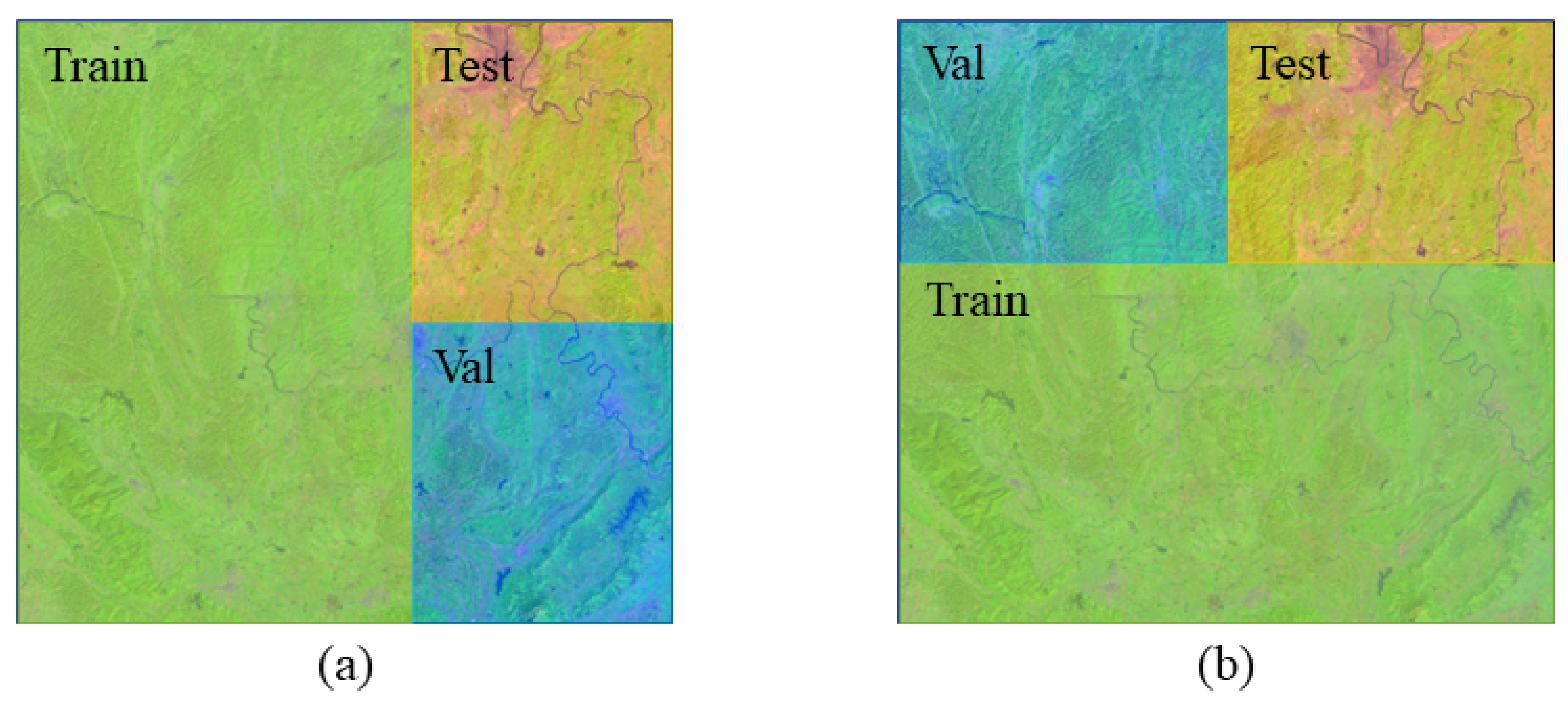
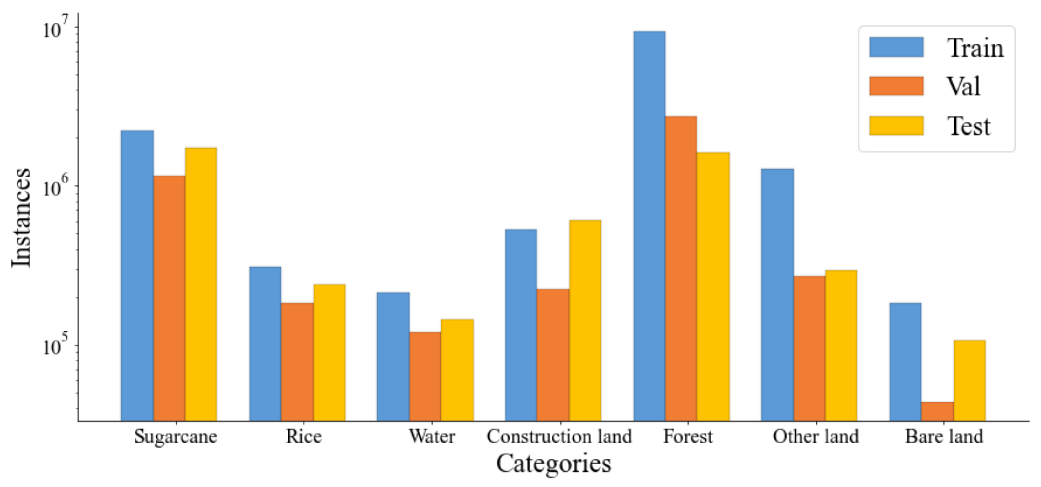
In this study, a multispectral image covering the study area taken by the Landsat 8 satellite on 2 October 2019, with a resolution of 30 m, containing 11 bands, was used as the data source. Landsat 8 carries the Operational Land Imager and Thermal Infrared Sensor. The Operational Land Imager includes nine bands with a spatial resolution of 30 m, including a 15 m panchromatic band, where the imaging width is 185 × 185 km. The Thermal Infrared Sensor includes two separate thermal infrared bands with a resolution of 100 m. To obtain more effective image information, the images were preprocessed with ENVI software for geolocation, radiometric calibration, atmospheric correction, mosaicking, and cropping. After that, the sample library data were obtained by a combination of indoor supervised classification and field validation, which involved 22,868,430 samples. The dataset was divided as shown in Figure 2; dataset I was used for all experiments and dataset II was used to further verify the validity of SA-UNet. As shown in Figure 3, 60% of the samples were used for training, 20% for validation, and 20% for testing. To ensure each slice did not contain background, a small range of intersection areas was included in the training, validation, and test sets, which did not affect the results. To increase the diversity of training samples, a sliding window method was used to crop the images into 256 × 256 blocks, with the window sliding 32 pixels each time to ensure 224 overlapping pixels between blocks of images with close boundaries. The training set was cropped to 3060, 256 × 256 samples, the validation set was cropped to 72, 256 × 256 samples, and the test set was cropped to 72, 256 × 256 samples.

2.3. Analysis of the Influence of Different Level Features on the Land Cover Classification of Landsat 8 Images

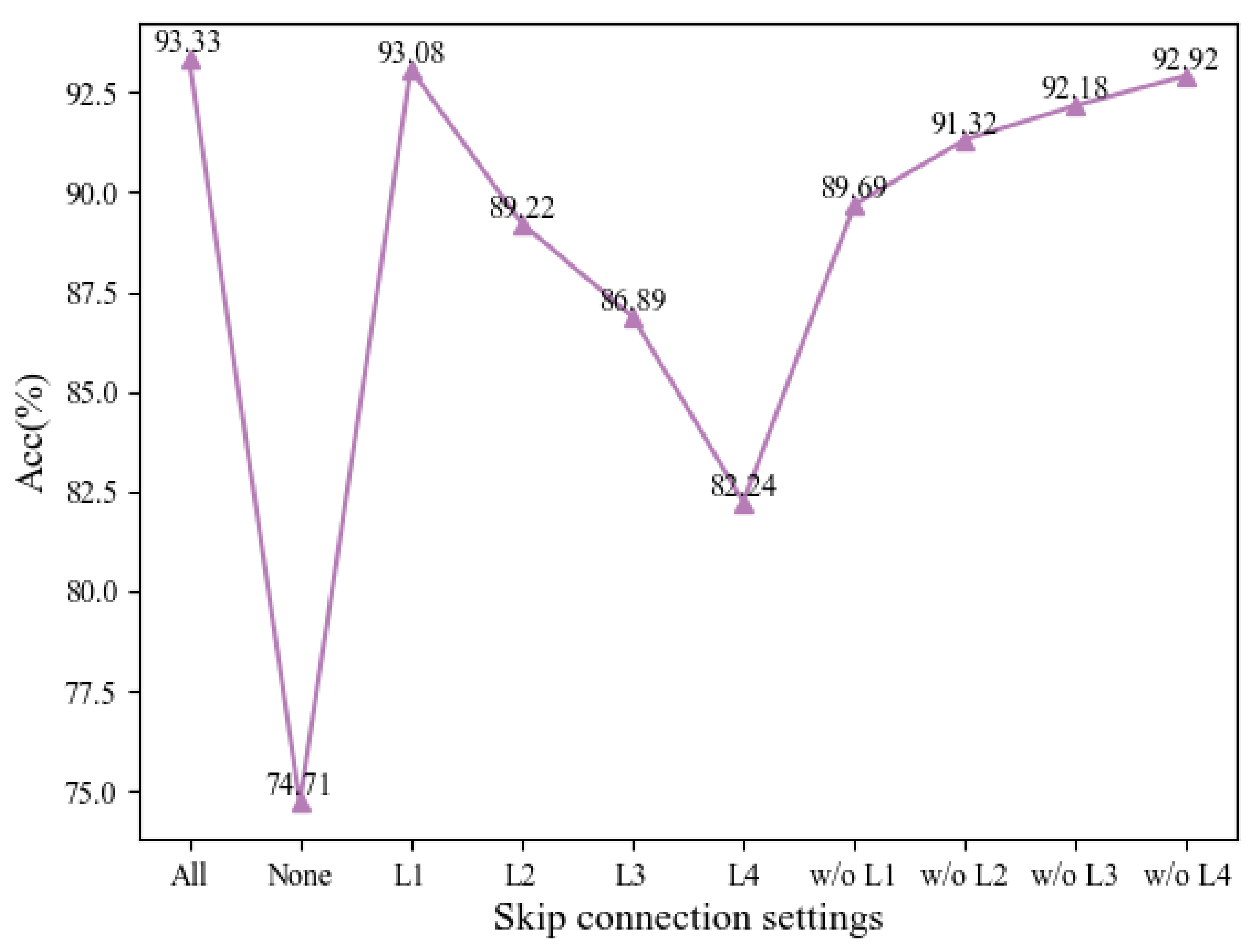
U-Net (Figure 4) fuses features from different levels through skip connections so that the features of the encoder and decoder complement each other and recover more detailed information from the image [40]. U-Net++ [28] and U-Net3+ [41] use dense skip connections to achieve a full-scale U-Net. However, for Landsat 8 remote sensing images, denser skip connections do not necessarily lead to higher-accuracy classification results of ground objects: some skip connections may even have a negative impact. Therefore, the data from the study area were used to deeply analyze the impact of U-Net on the classification results of Landsat 8 images using different feature levels. The results are shown in Figure 5. (1) The U-Net without skip connections performed the worst, and the overall accuracy is 18.62% lower than the original U-Net. The decoder of ‘U-Net-None’ is not combined with the information of the encoder, only upsampling the feature map to restore the input size, and the information is significantly lost. (2) The different levels of features provided different contributions to the classification results: the accuracy of U-Net was 93.33%, the accuracy of U-Net-L1 was 93.08%, and the accuracy of U-Net-w/o L1 was 89.69%. Compared with L2, L3, and L4, L1 contributed the most to U-Net. Therefore, shallow features play an important role in the classification results. (3) U-Net-w/o L1 was 3.39% less accurate than U-Net-L1: only the first-level skip connections positively affected U-Net. When removing the second-, third-, and fourth-level skip connections alone, the accuracy did not drop, but instead increased, especially when the fourth-level skip connections were moved. The reason for this finding may be that the high-level features were not suitable for feature fusion. Therefore, features at different levels provided different contributions to the results. So, the expressive power of features with large contributions should be enhanced, and that of features with negative effects should be reduced. These results demonstrate the importance of enhancing shallow feature representation as well as improving semantic information.

2.4. SA-UNet

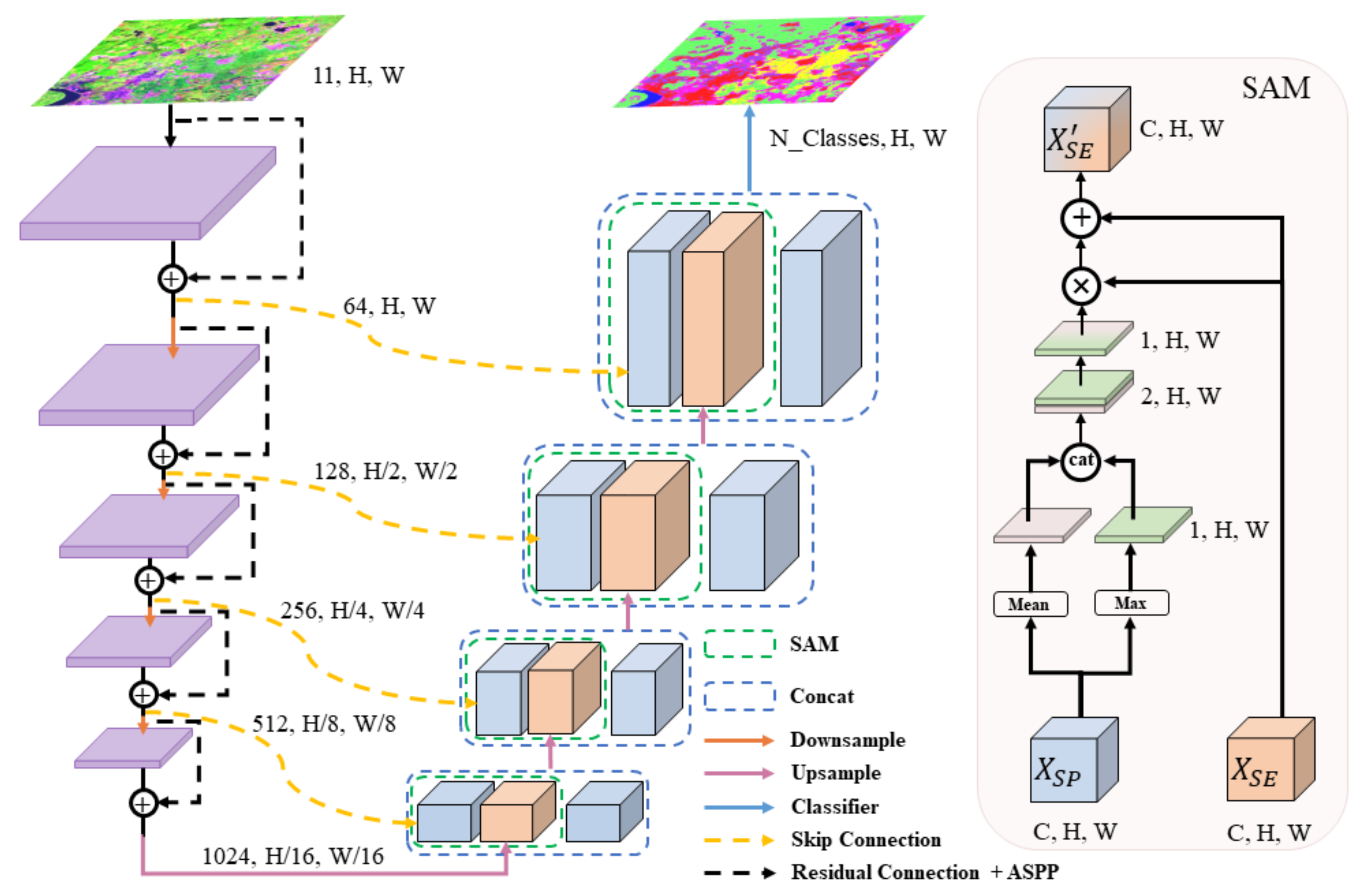
In response to the problems identified in Section 2.3, the SA-UNet network structure was designed. The overall structure of SA-UNet is shown in Figure 6. SA-UNet includes two parts, an encoder and a decoder, which are combined through a y skip connection. The overall structure includes five residual modules, five ASPP modules, and four SAMs. Each convolutional layer of the backbone network is accompanied by a batch normalization layer and a ReLU layer. In the ASPP module, the null convolution is accompanied by a ReLU layer with a pooling size of 2 × 2, a convolutional kernel size of 2 × 2, and a step size of 2 × 2 for the transposition convolution.

2.4.1. ASPP

The ASPP module is shown in Figure 7, having a total of five branches in parallel. The 1st branch is a 1 × 1 ordinary convolutional layer; the 2nd, 3rd, and 4th branches use 3 × 3 dilated convolutions with dilation coefficients of 6, 12, and 18, respectively. The 5th branch adopts global average pooling, outputs (batchsize, in_channel, 1, 1), then changes the number of channels through 1 × 1 convolution, and finally uses bilinear interpolation to restore the feature map to the input size. The features obtained from the five branches are superimposed in dimension. There are five times as many output channels as input channels. The number of channels is changed by a 1 × 1 convolution to obtain the final output. The ASPP module uses an inflated convolution that adds voids to the normal convolution to expand the perceptual field, which alleviates the problem of decreases in spatial resolution due to the maximum pooling layer [42]. Therefore, through the receptive field and integrating multiscale features, the expressive ability of shallow features is enhanced. In addition, by fusing the residual structure and combining the ASPP module with the backbone network, the shallow and deep features are deeply fused, and the characteristics of the shallow and deep features are more effectively used.

2.4.2. SAM

The spatial attention mechanism focuses on where the information is located in the current task. In remote sensing images, the types of ground objects are diverse and their distributions are complex, and the use of SAM to aggregate semantic information and spatial information is a way to improve the distinction of ground objects. SAM draws on the idea of CBAM [31], where SAM first uses the feature map of spatial information path ( X S P ) to obtain the spatial feature weight map W S , and then multiplies the semantic information path feature map ( X S E ) by the corresponding spatial location to obtain representative features, and then sums them with X S E at the corresponding spatial location to obtain X S E .
To learn the spatial weights, first obtain two channel information feature descriptors, X S P a v g S R 1 × H × W and X S P m a x S R 1 × H × W , by using average pooling and max pooling on the channel axis of the feature map. Then X S P a v g S and X S P m a x S are concatenated, and a 7 × 7 convolution is used to generate the spatial attention map. Finally, the spatial attention map is scaled to 0~1 using the sigmoid function to obtain the spatial feature weight map W S . The spatial attention is calculated as follows:
X S E = σ f 7 × 7 AvgPool X S P ; MaxPool X S P × X S E + X S E = σ f 7 × 7 X S P a v g S , X S P m a x S × X S E + X S E = W S × X S E + X S E
where ( X S E ) and ( X S P ) represent the semantic and spatial information path feature maps, respectively; σ represents the sigmoid function; f 7 × 7 represents the convolutional operation with a convolution size of 7 × 7 ; AvgPool represents the average pooling of each pixel along the channel axis; and MaxPool represents the max pooling of each pixel along the channel axis.

2.4.3. Loss Function

Due to the superior performance of the cross-entropy loss function, for multiclassification tasks, the cross-entropy loss function is usually chosen as the loss function. The cross-entropy loss function compares the predicted class with the target class for each pixel, and is expressed as follows:
L = 1 N i c = 1 M y i c log p i c
where M represents the number of classes; y i c is the sign function (0 or 1): when the true class of sample i is equal to c, y i c takes a value of 1, and otherwise, it takes 0. p i c is the predicted probability that the observed sample i belongs to class c.

2.5. Evaluation Metrics

To evaluate the semantic segmentation of remote sensing images, four evaluation metrics based on the confusion matrix were used: Accuracy, which is the ratio of the number of correct predictions to the number of all predictions; Precision, which is the ratio of correct predictions to positive classes to all predictions to positive classes; mean intersection over union (mIoU), which averages the intersection over union (IoU) of each class, so as to more accurately reflect the overall prediction performance of the model compared to IoU; and the Kappa coefficient, which is an indicator of the consistency of two variables. The formulas for these quantitative assessment metrics are as follows:
A c c u r a c y = T P + T N T P + F N + F P + T N
P r e c i s i o n = T P T P + F P
m I o U = 1 n i = 1 n a i i j = 1 n a i j + j = 1 n a j i a i i
K a p p a = p o p e 1 p e
where TP is the positive category that is classified accurately, FP is the negative category that is misclassified as positive, TN is the negative category that is classified accurately, FN is the positive category that is misclassified as negative, p o is the overall precision, and p e is the number of the misclassified samples divided by the total number of samples.

2.6. Experimental Environment

In the experiments, ENVI software was used to obtain sample points from the outdoor sampling and the learned prior knowledge to label the regions of interest. A supervised classification method was used to obtain the label maps needed for the experiments. In the training phase, the cross-entropy loss function was selected, the batchsize was set to 8, the maximum epoch was 20, and Adam was selected as the optimizer. The Adam optimizer uses a gradient descent algorithm, which has an adaptive learning rate, and the momentum gradient descent algorithm, which can alleviate the effects of the gradient oscillation problem. The initial learning rate was 0.01, and the learning rate decayed to 0.1 times the original rate every five iterations. All experimental code was implemented by Python 3.9 in pytorch 1.10.2, and the model was trained in win10+i5-8500CPU+NVIDIA GeForce RTX 3060 12 G GPU.

3. Results

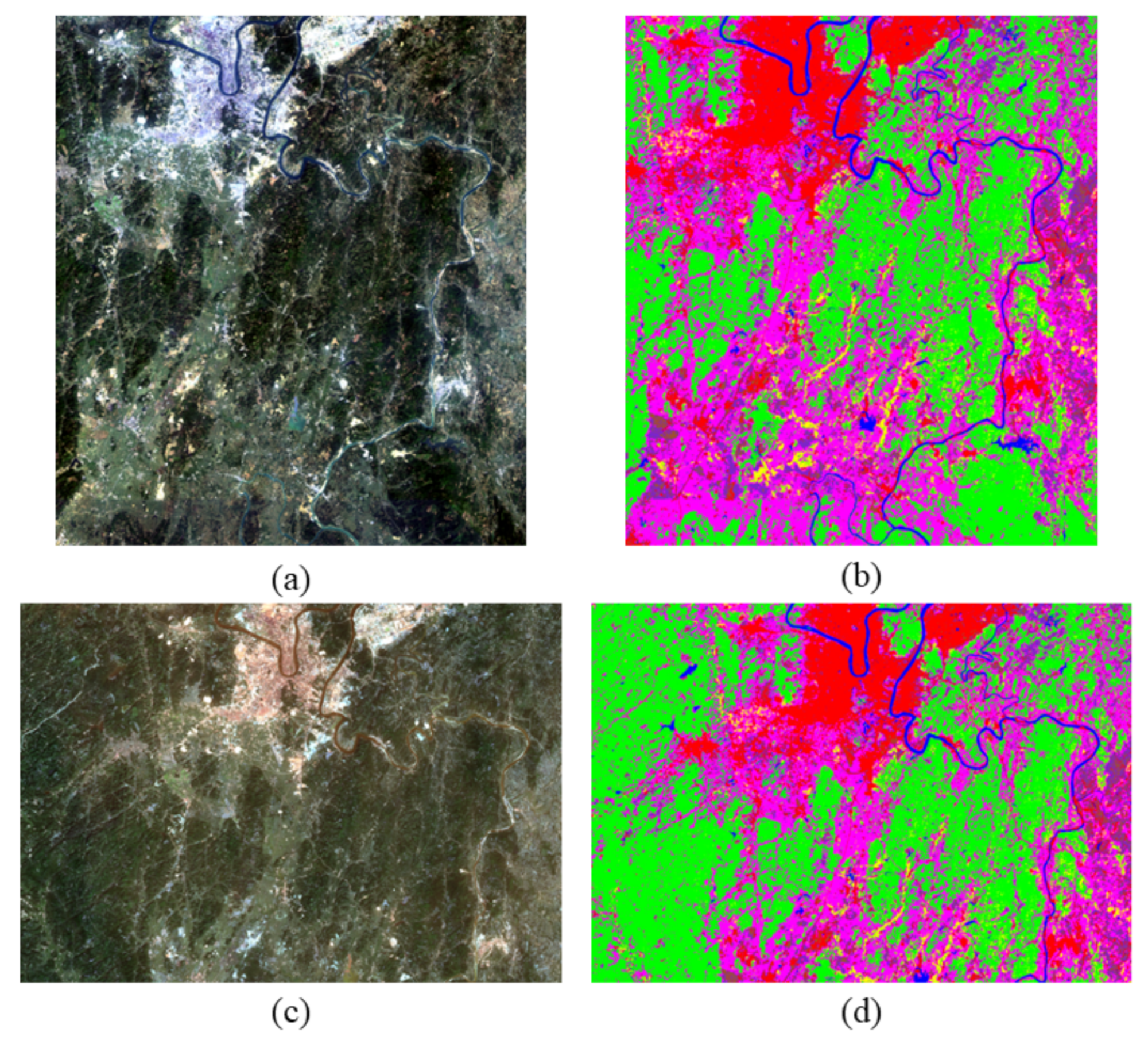
The details of the sample pool in the study area are shown in Table 1 and Table 2, where 60% was used for training, 20% for validation, and 20% for testing. The following experiments were conducted using the sample pool data in Table 1 and Table 2. Due to space limitations, construction land, other land, and bare land are abbreviated as CL, OL, and BL, respectively. The test set true-color images and labeled maps are shown in Figure 8.
In order to select a suitable learning rate, the proposed model was experimented in this paper with learning rates set to 0.1, 0.01 and 0.001, respectively, and the experimental results are shown in Table 3, where the values of Acc, mIoU, and Kappa were maximal for the learning rate = 0.01.

3.1. Ablation Study

To evaluate the proposed network structure and the performance of two important modules, ablation experiments were performed on the dataset I in the study area using U-Net as the base network.
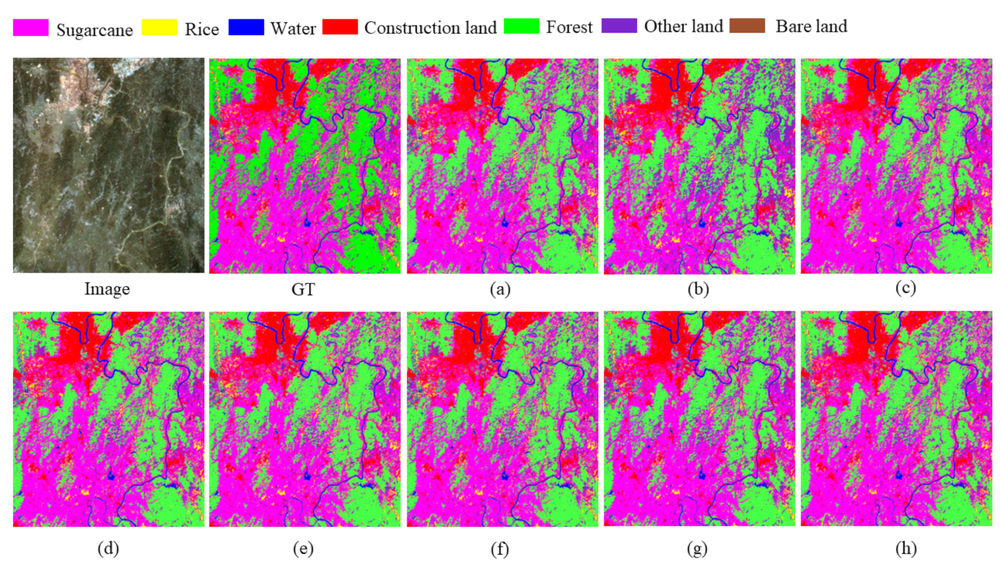
(1) Effect of ASPP: The results are shown in Table 4. The ASPP module was introduced into U-Net in the form of residuals to segment the test set images. The overall accuracy increased by 2.92%, the mIoU increased by 7.35%, and the Kappa coefficient increased by 4.06%. In particular, the recognition accuracy of rice (+17.03%), other land (+5.57%), and bare land (+6.53%) considerably improved. The recognition accuracy rates of sugarcane (+1.63%), water (+3.48%), construction land (+1.6%), and forest (+1.89%) also improved. This verified the effectiveness of integrating the ASPP module into U-Net in the form of residuals. As shown in the first row in Figure 9, the bridges in the construction land were segmented after U-Net was added to ASPP, whereas U-Net was not implemented. The second row in Figure 9 shows that the U-Net+ASPP segmentation of rice was more accurate than that of U-Net, and sugarcane, rice, and forest were more easily and accurately segmented. The results showed that combining ASPP with residual units enables the network to focus not only on global information, but also on detailed information.
(2) Effect of SAM: The results are shown in Table 4 for the combination of SAM with U-Net for the test set images. The accuracy increased by 2.2%, the mIoU increased by 4.68%, and the Kappa coefficient improved by 3.07%. SAM combined spatial with semantic information and increased the network recognition rate of different category differences for sugarcane (+0.77%), rice (+14.75%), water (+2.75%), construction land (+0.75%), forest (+1.8%), other land (+5.15%), and bare land (+2.13%). The detection accuracies of sugarcane and rice decreased by 1.4% and 10.16%, respectively. The mixing matrix showed that the number of misclassified samples within the groups of sugarcane, rice, and forest decreased, and the number of misclassified samples between the groups decreased. Comparing the data in Table 4 shows that SAM had the most obvious effect on forest recognition accuracy. With the addition of SAM, the network more easily distinguished between categories with large between-group differences, but less easily distinguished between categories with small within-group differences. The first row of Figure 9 shows that the inclusion of SAM facilitated distinguishing construction land from water; the second row of Figure 9 shows that SAM was more effective than U-Net for the segmentation of concentrated rice planting areas, but did not improve the recognition of areas where rice planting distribution was scattered, compared with U-Net. The results showed that SAM enhanced the intergroup differences and improved the segmentation between features with large differences.
(3) Effect of ASPP+SAM: Table 4 shows that ASPP, SAM, and U-Net set not only reduced the misclassification within the group, but also reduced the misclassification between groups. Sugarcane (+1.59%), rice (+19.84%), water (+3.45%), construction land (+1.59%), other land (+7.28%), and bare land (+6.68%) recognition accuracies increased, showing the most impact on rice and other land recognition. As shown in the third row, the contour of the other land segmented by U-Net+ASPP+SAM was more accurate, as was the extraction of small-area rice. Therefore, SA-UNet can focus on information at different scales to increase the accuracy of the classification results of ground objects. Although the accuracy of UNet+ASPP+SAM is the same as that of UNet+ASPP, the corresponding mIoU and Kappa coefficients are a bit higher for the former.

3.2. Comparison of Multiple Methods

To evaluate the performance of SA-UNet in feature coverage classification, comparative experiments and analyses were conducted with U-Net [22], U-Net++ [28], SAR-UNet [42], Res-UNet++ [24], Attention-UNet [18], UCTransNet [29], and Swin-UNet [39]. U-Net++ provides an improvement in full-scale feature fusion based on U-Net, SAR-UNet, and Res-UNet++. In Attention-UNet, an attention mechanism is added on the basis of U-Net. UCTransNet is a channel-wise cross-fusion transformer that functions on the basis of joining U-Net. Swin-UNet is a U-shaped network composed of pure Swin-transformer. The proposed algorithm SA-UNet incorporates ASPP into U-Net in the form of residuals, and combines semantic and spatial information through a spatial attention mechanism in the decoder process. None of the above methods were pretrained.
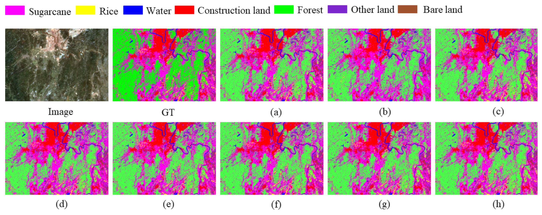
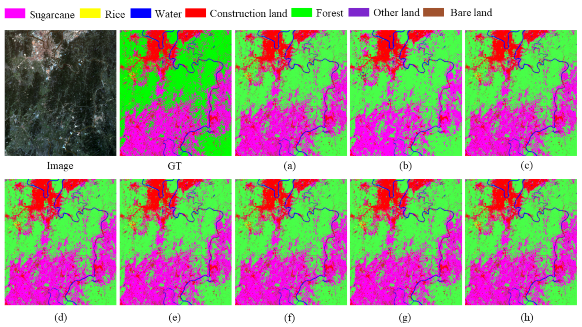
The segmentation results of the different algorithms on the test set from the dataset I are shown in Table 5. For three evaluation metrics (Acc, mIoU and Kappa), the proposed SA-UNet outperformed the other algorithms in the three metrics of Acc (96.25%), mIoU (89.33%) and Kappa (94.84%). The segmentation accuracy of SA-UNet for rice (83.21%), water (97.46%), construction land (97.02%), other land (95.71%) and bare land (88.45%) is also the highest compared with the other algorithms mentioned above. U-Net++ used a full-scale fusion approach, but the generalization ability of UNet++ became worse compared to U-Net. SAR-UNet achieved the highest segmentation accuracy for sugarcane, at 98.74%, but its segmentation results for rice (−7.13%), construction land (−5.67%) and other land (−8.79%) were inferior to those of U-Net. Res-UNet++ only slightly improved the accuracy of the segmentation of sugarcane (+1.27%), water (+0.58%) and forest (0.14%) compared with U-Net, although Res-UNet++ had slightly higher Acc and Kappa than U-Net, but a lower mIoU value.Attention-UNet has similar performance compared to U-Net. UCTransNet slightly improves the segmentation of Water (0.43%), and Construction land (0.48%), Other land (1.95%) and bare land (0.77%) compared to UNet, but unsatisfactory results for the rice. Swin-UNet received a lower Acc (−0.09%), mIoU (−4.7%), and Kappa (−1.24%) than U-Net. SA-UNet performed the best overall, producing the improvement in sugarcane (+1.59%), rice (+19.84%),water (+3.45%), forest (+1.21%), other land (+7.28%), and bare land (+6.68%) segmentation, indicating that SA-UNet provides advantages in the land cover classification of Landsat 8 remote sensing images. Table 6 shows the segmentation results of different methods for the test set of dataset II. Acc (96.62), mIoU (89.20) and Kappa (95.16) of SA-UNet are still the highest compared with other methods.
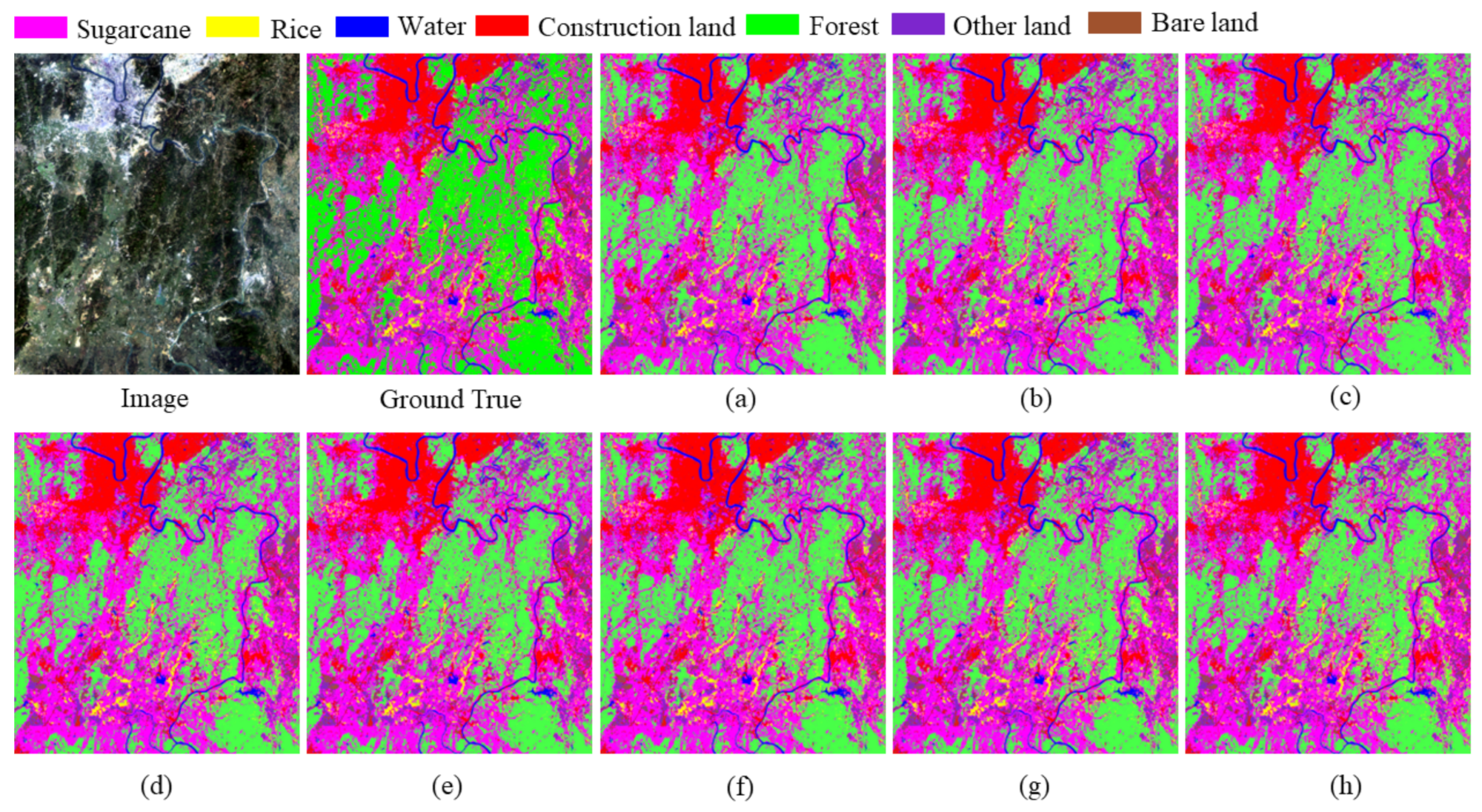
Figure 10 shows the segmentation results of the remote sensing images from the test set in the study area by different methods. Generally, the image segmentation results of each algorithm were almost the same. The proportions of construction land, forest, and sugarcane in the test set were relatively large; the planting of sugarcane and rice was more concentrated; and the proportions of other land types were smaller. The segmentation result graph of the test set is shown in Figure 11, and the effectiveness of SA-UNet can be reflected by combining Table 6 with Figure 11 (for the following experiments, except for Figure 11 and Table 6, all of experiments are with dataset I).
Comparing Figure 10 with Figure 12 shows that the differences between the algorithms are mainly reflected in the local area. From local observations, rice distribution was more scattered in this image, indicated by the yellow and red boxes; for this scattered rice distribution, only the proposed algorithm produced results most similar to the ground truth. The other algorithms all produced visible errors. SAR-UNet poorly segmented rice and mixed rice with forest. As seen from the colored baskets, some networks experienced some difficulty in identifying bridges over rivers: U-Net, UNet++, and UCTransNet failed to segment the bridges from the water. SAR-UNet, Res-UNet++, Attention-UNet, and Swin-UNet were also unsatisfactory, and only SA-UNet showed some minor differences from ground truth. As seen from the black box, U-Net, U-Net++, SAR-UNet, and UCTransNet were unable to distinguish sugarcane from forest in detail, easily misclassifying sugarcane as forest. Swin-UNet and SA-UNet were more accurately able to distinguish sugarcane and forest.

3.3. Land Use Change in Study Area

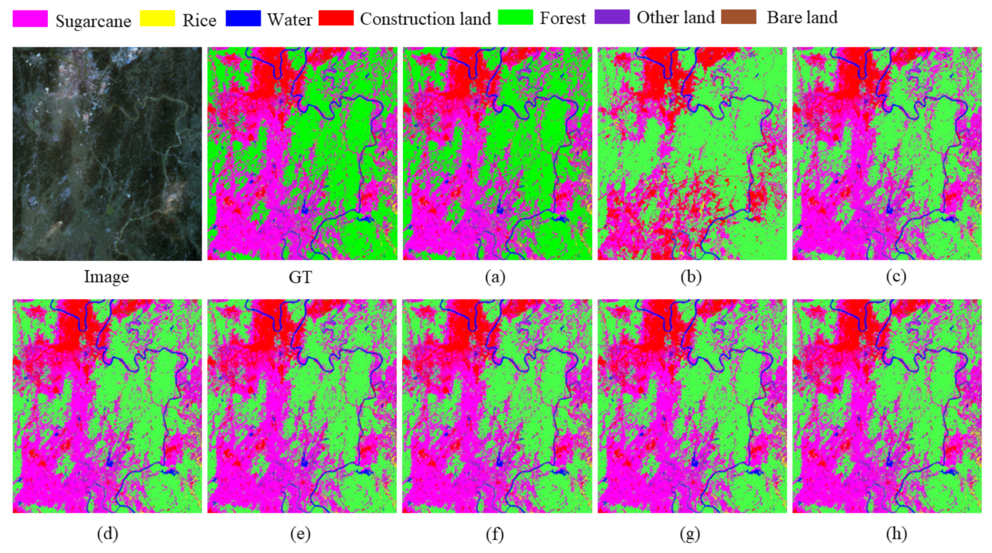
In this study, four issues of Landsat 8 series remote sensing images dated 13 October 2015, 28 October 2017, 2 October 2019 and 13 October 2021 were downloaded from the USGS website (https://earthexplorer.usgs.gov/ accessed on 1 January 2021) to classify the land cover of the study area. Higher-resolution imagery, field collection data, and a priori knowledge were used for supervised classification to obtain the 2015, 2017, 2019, and 2021 sample base data for the study area. The method of Table 5 and the dataset I were used to analyze the four phases of images. Finally, the proposed algorithm was used to classify and evaluate the four phases of images in turn for land cover classification. The results of the multiple methods segmentation of the test sets for 2015, 2017, 2019 and 2021 are shown in Figure 10 and Figure 13, Figure 14 and Figure 15, respectively. As shown by the evaluation metrics in Table 5 and Table 7, Table 8 and Table 9, the Acc, mIoU, and Kappa values of the four-phase images met the needs of the study.
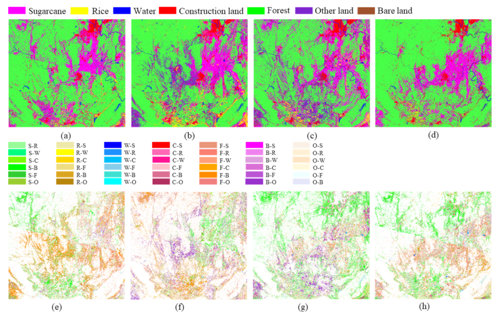
The spatial distributions of land use and land use changes are shown in Figure 16. From the spatial analysis of land use distribution, the study area was mostly covered by forest, the planting areas of sugarcane and rice were relatively concentrated, sugarcane was the most widely planted among crops, the main rivers ran through the whole study area, large cities were mainly distributed on both sides of the main rivers, and lakes and reservoirs were randomly distributed throughout the whole study area. From the analysis of land use changes, the conversions of sugarcane plantation areas into other land, forest plantation areas into other land, and bare land into other land were more common.
The land use and land use change rate for the seven-year period are shown in Table 10. Combining the results in Table 10 with those of Figure 16, the proportion of forested land cover area in the study area was found to be the largest among the four images, followed by sugarcane and construction land. From the analysis of land use change, the areas of two major crops, sugarcane and rice, changed the most every year. The area of bare land increased each year because, first, distinguishing bare land from freshly planted fruit trees and crops in Landsat 8 remote sensing images is difficult and, second, human activities. In 2019–2021, the water area changed by −60.2%, indicating that a drought occurred during the period, causing the reservoir as well as some tributaries to dry up. The overall change in construction land was small, with basically no change in large cities and sporadic changes in villages, various factories, and concrete floors. In 2019–2021, other arable land (−79.99%) and sugarcane (−28.16%) mainly transformed into forest (+19.74%), increasing the forest area to that observed in 2015, proving that green ecological awareness is increasing.

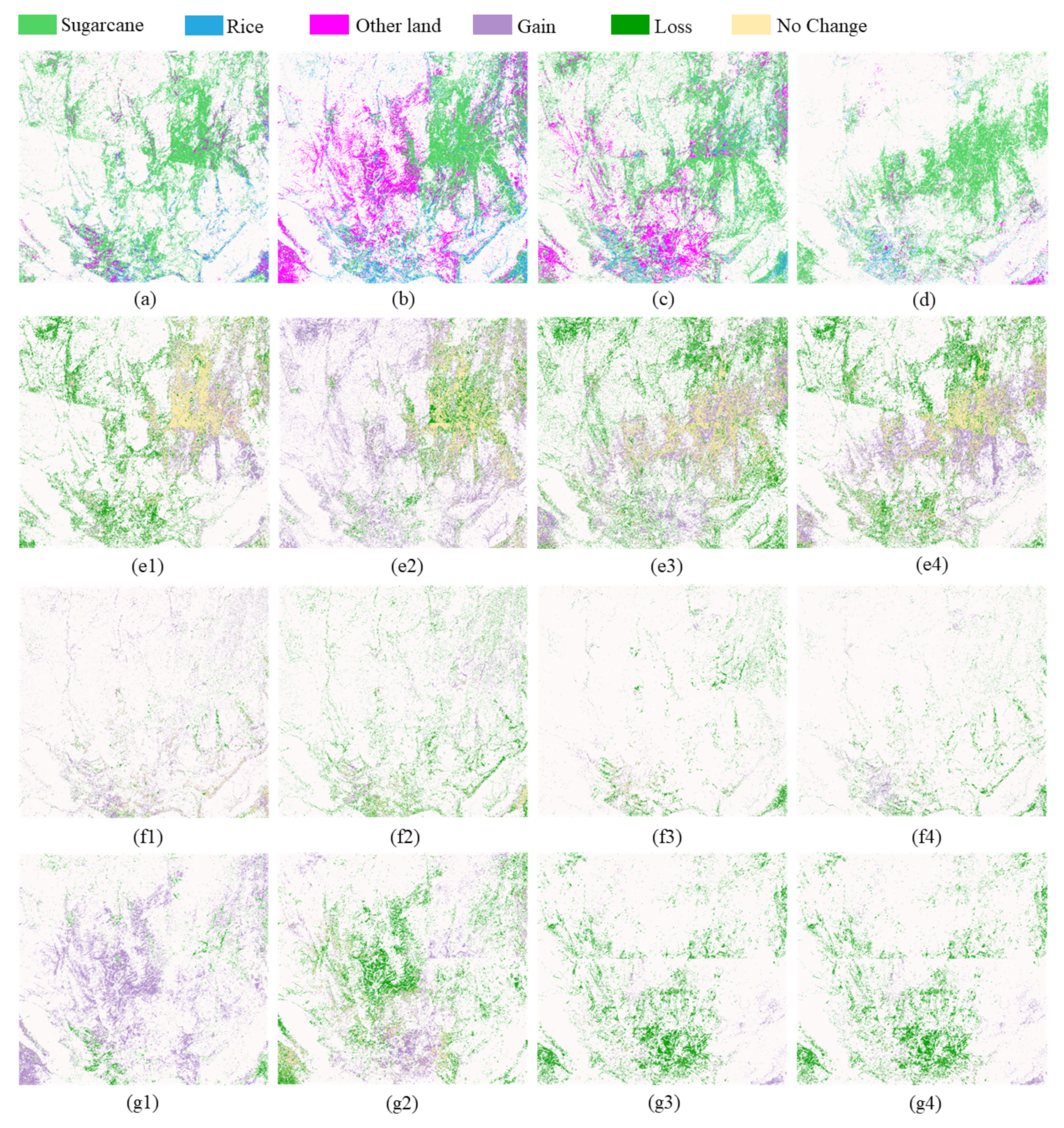
3.4. Crop Land Use Change

The classification results of remote sensing images in 2015, 2017, 2019 and 2021 show that the proposed algorithm increases the classification accuracy of sugarcane, rice, and other land. Therefore, the proposed algorithm was used to monitor the dynamic changes in crops over a seven-year period. The crop acreage in the four periods in the study area was analyzed and compared, and the classification results and the dynamic changes in crops are shown in Figure 17. The statistics of the results of monitoring the area for regional changes in crop cultivation are shown in Table 10, which show that the area under sugarcane cultivation was 3725.88 km 2 in 2015, 2780.16 km 2 in 2017, 4491 km 2 in 2019, and 3504.14 km 2 in 2021. The area planted with sugarcane decreased by 25.38% in 2015–2017, increased by 61.54% in 2017–2019, decreased by 28.16% in 2019–2021, and decreased by 5.95% in 2015–2021. The area under sugarcane cultivation mainly transformed into forest, rice, and other land. Rice cultivation area was 596.19 km 2 in 2015, 1384.95 km 2 in 2017, 633.17 km 2 in 2019, and 295.3 km 2 in 2021, increasing 132.3% in 2015–2017, decreasing 54.28% in 2017–2019, decreasing 60.2% in 2019–2021, and decreasing 50.49% in 2015–2021. A general trend of decreasing rice growing area was observed; usually, rice fields were converted to sugarcane along with other land. Because the number of farmers cultivating the land is gradually decreasing, the land is being leased to contractors who convert the rice fields to grow fruit, sugarcane, or other crops. The area under other crops was 491.38 km 2 in 2015, 2405.03 km 2 in 2017, 1581.84 km 2 in 2019, and 316.55 km 2 in 2021. The area under other crops increased by 382.57% in 2015–2017, decreased by 34.22% in 2017–2019, decreased by 79.99% in 2019–2021, and decreased by 36.48% in 2015–2021. The area for other crops gradually transformed into sugarcane and forest land.

4. Discussion

In Landsat 8 remote sensing image feature classification, U-Net is more accurate than U-Net++. Section 2.3 shows that not all skip connections are beneficial to the classification result, so the strategy of full-scale fusion adopted by U-Net++ has a negative effect on the overall feature coverage classification accuracy. However, full-scale fusion has a better effect on improving intergroup differences, so when the differences in feature types are small, ablation experiments must be conducted on skip connections to select the most appropriate scale features for fusion. When the differences in feature type are large, full-scale fusion is beneficial for increasing intergroup differences. The channel attention mechanism increases the SAR-UNet attention to sugarcane, which leads to a sugarcane segmentation accuracy of 98.74%. Although SAR-UNet includes ASPP modules in the transition layer of the network to increase semantic information, Section 2.3 shows that increasing the expressiveness of shallow features is more beneficial in the classification of Landsat 8 remote sensing images. Res-UNet++ has a similar structure to SAR-UNet, except that Res-UNet++ has a spatial attention mechanism in the decoder part to enable focus on the key regions of the feature maps. Unlike the spatial attention mechanism module used in this study, Res-UNet++ combines two feature maps of different sizes to generate spatial attention weights and obtain new semantic information. This is consistent with the idea of Attention-UNet, but Attention-UNet reduces the redundant features of hopping connection transmission and highlights the salient features of specific local regions. The analysis of the results shows that Res-UNet++ is slightly more accurate than Attention-UNet. The structures of SAR-UNet, Res-UNet++, and Attention-UNet and the results show that adding channel attention to the encoder and then adding spatial attention to the decoder little impacts the classification results. UCTransNet uses the CTrans module instead of traditional skip connections. CTrans uses transformer to cross-fertilize multiscale information on the features of the four different levels of U-Net, which reduces the negative effects produced by some skip connections. CTrans works best for the segmentation of two types of features with the most obvious characteristics, namely forest and construction land, and may produce accurate results if used for road segmentation. Swin-UNet improves Swin-Transformer by using a U-shaped structure to achieve semantic segmentation. Because the continuous attentional layer structure of Swin-Transformer can substantially improve the expression of the model, the segmentation results for forest of Swin-UNet were better than those of the other comparison methods. In the 30 m high-resolution remote sensing image land cover classification task, the shallow features strongly influenced the experimental results, but as the network deepened, the spatial resolution was reduced and spatial information was dispersed. Therefore, the proposed SA-UNet uses different scales of cavity convolution to expand the perceptual field, and enables the multiscale fusion of features to increase the ability to express shallow features. In addition, SA-UNet fuses shallow with deep features by fusing residual modules to effectively use the characteristics of both shallow and deep features. To integrate more spatial information into the upsampling feature map, the feature map obtained by jump connection is fused with the upsampling feature map using the spatial attention module to enhance the combination of spatial and semantic information. Compared with UNet, SA-UNet improved the classification accuracy of all ground objects. As rice is a major food crop, accurately extracting rice growing areas from remote sensing images is important, but the rice segmentation accuracy of the proposed method is still insufficient and needs further improvement.

5. Conclusions

In this study, the main focus was improving the ability to express shallow features in remote sensing images, enhancing the effective combination of spatial and semantic information, to obtain global contextual information and improve the segmentation effect of ground objects. In this study, U-Net and an ASPP module were fused by means of residuals. This fusion not only expands the perceptual field through the convolution of cavities of different sizes, promotes the fusion of multiscale features, and enhances the expression ability of shallow features, but also enables the deep fusion of shallow and semantic features, which mitigates the effects of the problem where local complex feature types interfere with each other. In addition, a spatial attention module was used to fuse the feature maps obtained from jump connections with the upsampled feature maps, which alleviates the problem caused by the inadequate use of spatial information in the upsampling process. The results showed that the proposed SA-UNet produced relatively more accurate feature classification results from Landsat 8 remote sensing images in the study area compared with U-Net, U-Net++, SAR-UNet, Res-UNet++, Attention-UNet, UCTransNet, and Swin-UNet with an accuracy rate of 96.25%. For future work, the features of jump connections should be further optimized so that the model can enhance both inter and intragroup differences.

Author Contributions

Conceptualization, X.F. and C.Y.; methodology, C.Y. and X.F.; software, C.Y., X.F. and J.F.; validation, C.Y., X.F. and J.F.; formal analysis, C.Y., X.F. and J.F.; investigation, C.Y. and X.F.; resources, X.F. and J.F.; data curation, C.Y. and N.W.; writing—original draft preparation, C.Y.; writing—review and editing, C.Y., X.F., J.F. and N.W. All authors have read and agreed to the published version of the manuscript.

Funding

This research was funded by the National Natural Science Foundation of China under Grant (62001129) and the Guangxi Natural Science Foundation under Grant (2021GXNSFBA075029).

Data Availability Statement

The SA-UNet and 2019 data set in the study area will be available at https://github.com/Yancccccc/SA-UNet accessed on 9 June 2022.

Conflicts of Interest

The authors declare no conflict of interest.

Abbreviations

ASPPAtrous spatial pyramid pooling
SVMSupport vector machine
CNNConvolutional neural network
NLPNatural language processing
ViTVision Transformer
SAMSpatial attention module
CRFConditional random fields
mIoUMean intersection over union
CLConstruction land
OLOther land
BLBare land

References

  1. Hu, Q.; Yin, H.; Friedl, M.A.; You, L.; Li, Z.; Tang, H.; Wu, W. Integrating coarse-resolution images and agricultural statistics to generate sub-pixel crop type maps and reconciled area estimates. Remote Sens. Environ. 2021, 258, 112365. [Google Scholar] [CrossRef]
  2. Lorenz, S.; Ghamisi, P.; Kirsch, M.; Jackisch, R.; Rasti, B.; Gloaguen, R. Feature extraction for hyperspectral mineral domain mapping: A test of conventional and innovative methods. Remote Sens. Environ. 2021, 252, 112129. [Google Scholar] [CrossRef]
  3. Li, B.; Xie, X.; Wei, X.; Tang, W. Ship detection and classification from optical remote sensing images: A survey. Chin. J. Aeronaut. 2021, 34, 145–163. [Google Scholar] [CrossRef]
  4. Bioucas-Dias, J.M.; Plaza, A.; Camps-Valls, G.; Scheunders, P.; Nasrabadi, N.; Chanussot, J. Hyperspectral Remote Sensing Data Analysis and Future Challenges. IEEE Geosci. Remote Sens. Mag. 2013, 1, 6–36. [Google Scholar] [CrossRef] [Green Version]
  5. Tong, X.Y.; Lu, Q.; Xia, G.S.; Zhang, L. Large-Scale Land Cover Classification in Gaofen-2 Satellite Imagery. In Proceedings of the IGARSS 2018—2018 IEEE International Geoscience and Remote Sensing Symposium, Valencia, Spain, 22–27 July 2018; pp. 3599–3602. [Google Scholar] [CrossRef] [Green Version]
  6. Zhang, B.; Wu, Y.; Zhao, B.; Chanussot, J.; Hong, D.; Yao, J.; Gao, L. Progress and Challenges in Intelligent Remote Sensing Satellite Systems. IEEE J. Sel. Top. Appl. Earth Obs. Remote Sens. 2022, 15, 1814–1822. [Google Scholar] [CrossRef]
  7. Crowther, T.W.; Glick, H.B.; Covey, K.R.; Bettigole, C.; Maynard, D.S.; Thomas, S.M.; Smith, J.R.; Hintler, G.; Duguid, M.C.; Amatulli, G.; et al. Mapping tree density at a global scale. Nature 2015, 525, 201–205. [Google Scholar] [CrossRef] [PubMed]
  8. Gao, Q.; Lim, S.; Jia, X. Spectral–Spatial Hyperspectral Image Classification Using a Multiscale Conservative Smoothing Scheme and Adaptive Sparse Representation. IEEE Trans. Geosci. Remote Sens. 2019, 57, 7718–7730. [Google Scholar] [CrossRef]
  9. Zhang, S.; Kang, X.; Duan, P.; Sun, B.; Li, S. Polygon Structure-Guided Hyperspectral Image Classification with Single Sample for Strong Geometric Characteristics Scenes. IEEE Trans. Geosci. Remote Sens. 2022, 60, 1–12. [Google Scholar] [CrossRef]
  10. Melgani, F.; Bruzzone, L. Support vector machines for classification of hyperspectral remote-sensing images. In Proceedings of the IEEE International Geoscience and Remote Sensing Symposium, Toronto, ON, Canada, 24–28 June 2002; Volume 1, pp. 506–508. [Google Scholar] [CrossRef]
  11. Jiang, Q.; Dong, Y.; Peng, J.; Yan, M.; Sun, Y. Maximum Likelihood Estimation Based Nonnegative Matrix Factorization for Hyperspectral Unmixing. Remote Sens. 2021, 13, 2637. [Google Scholar] [CrossRef]
  12. Feng, T.; Ma, H.; Cheng, X. Greenhouse Extraction from High-Resolution Remote Sensing Imagery with Improved Random Forest. In Proceedings of the IGARSS 2020—2020 IEEE International Geoscience and Remote Sensing Symposium, Waikoloa, HI, USA, 26 September–2 October 2020; pp. 553–556. [Google Scholar] [CrossRef]
  13. Baassou, B.; Mingyi, H.; Farid, M.I.; Shaohui, M. Hyperspectral image classification based on iterative Support Vector Machine by integrating spatial-spectral information. In Proceedings of the 2013 IEEE International Geoscience and Remote Sensing Symposium—IGARSS, Melbourne, Australia, 21–26 July 2013; pp. 1023–1026. [Google Scholar] [CrossRef]
  14. Zhang, P.; Ke, Y.; Zhang, Z.; Wang, M.; Li, P.; Zhang, S. Urban Land Use and Land Cover Classification Using Novel Deep Learning Models Based on High Spatial Resolution Satellite Imagery. Sensors 2018, 18, 3717. [Google Scholar] [CrossRef] [PubMed] [Green Version]
  15. Cao, K.; Zhang, X. An improved res-unet model for tree species classification using airborne high-resolution images. Remote Sens. 2020, 12, 1128. [Google Scholar] [CrossRef] [Green Version]
  16. Yan, C.; Fan, X.; Fan, J.; Wang, N. Improved U-Net Remote Sensing Classification Algorithm Based on Multi-Feature Fusion Perception. Remote Sens. 2022, 14, 1118. [Google Scholar] [CrossRef]
  17. Alam, F.I.; Zhou, J.; Liew, A.W.C.; Jia, X.; Chanussot, J.; Gao, Y. Conditional Random Field and Deep Feature Learning for Hyperspectral Image Classification. IEEE Trans. Geosci. Remote Sens. 2019, 57, 1612–1628. [Google Scholar] [CrossRef] [Green Version]
  18. John, D.; Zhang, C. An attention-based U-Net for detecting deforestation within satellite sensor imagery. Int. J. Appl. Earth Obs. Geoinf. 2022, 107, 102685. [Google Scholar] [CrossRef]
  19. Chen, L.C.; Zhu, Y.; Papandreou, G.; Schroff, F.; Adam, H. Encoder-decoder with atrous separable convolution for semantic image segmentation. In Proceedings of the European Conference on Computer Vision (ECCV), Munich, Germany, 8–14 September 2018; pp. 801–818. [Google Scholar]
  20. He, X.; Zhou, Y.; Zhao, J.; Zhang, D.; Yao, R.; Xue, Y. Swin Transformer Embedding UNet for Remote Sensing Image Semantic Segmentation. IEEE Trans. Geosci. Remote Sens. 2022, 60, 1–15. [Google Scholar] [CrossRef]
  21. Panboonyuen, T.; Jitkajornwanich, K.; Lawawirojwong, S.; Srestasathiern, P.; Vateekul, P. Transformer-Based Decoder Designs for Semantic Segmentation on Remotely Sensed Images. Remote Sens. 2021, 13, 5100. [Google Scholar] [CrossRef]
  22. Ronneberger, O.; Fischer, P.; Brox, T. U-net: Convolutional networks for biomedical image segmentation. In Proceedings of the International Conference on Medical Image Computing and Computer-Assisted Intervention, Munich, Germany, 5–9 October 2015; Springer: Berlin/Heidelberg, Germany, 2015; pp. 234–241. [Google Scholar]
  23. Lu, Y.; Shao, W.; Sun, J. Extraction of Offshore Aquaculture Areas from Medium-Resolution Remote Sensing Images Based on Deep Learning. Remote Sens. 2021, 13, 3854. [Google Scholar] [CrossRef]
  24. Jha, D.; Smedsrud, P.H.; Riegler, M.A.; Johansen, D.; Lange, T.D.; Halvorsen, P.; Johansen, H.D. ResUNet++: An Advanced Architecture for Medical Image Segmentation. In Proceedings of the 2019 IEEE International Symposium on Multimedia (ISM), San Diego, CA, USA, 9–11 December 2019; pp. 225–2255. [Google Scholar] [CrossRef] [Green Version]
  25. He, K.; Zhang, X.; Ren, S.; Sun, J. Deep residual learning for image recognition. In Proceedings of the IEEE Conference on Computer Vision and Pattern Recognition, Las Vegas, NV, USA, 27–30 June 2016; pp. 770–778. [Google Scholar]
  26. Petrovska, B.; Atanasova-Pacemska, T.; Corizzo, R.; Mignone, P.; Lameski, P.; Zdravevski, E. Aerial scene classification through fine-tuning with adaptive learning rates and label smoothing. Appl. Sci. 2020, 10, 5792. [Google Scholar] [CrossRef]
  27. Petrovska, B.; Zdravevski, E.; Lameski, P.; Corizzo, R.; Štajduhar, I.; Lerga, J. Deep learning for feature extraction in remote sensing: A case-study of aerial scene classification. Sensors 2020, 20, 3906. [Google Scholar] [CrossRef]
  28. Chen, C.; Fan, L. Scene segmentation of remotely sensed images with data augmentation using U-net++. In Proceedings of the 2021 IEEE International Conference on Computer Engineering and Artificial Intelligence (ICCEAI), Shanghai, China, 27–29 August 2021; pp. 201–205. [Google Scholar]
  29. Wang, H.; Cao, P.; Wang, J.; Zaiane, O.R. UCTransNet: Rethinking the skip connections in U-Net from a channel-wise perspective with transformer. arXiv 2021, arXiv:2109.04335. [Google Scholar] [CrossRef]
  30. Haut, J.M.; Paoletti, M.E.; Plaza, J.; Plaza, A.; Li, J. Visual Attention-Driven Hyperspectral Image Classification. IEEE Trans. Geosci. Remote Sens. 2019, 57, 8065–8080. [Google Scholar] [CrossRef]
  31. Woo, S.; Park, J.; Lee, J.Y.; Kweon, I.S. Cbam: Convolutional block attention module. In Proceedings of the European Conference on Computer Vision (ECCV), Munich, Germany, 8–14 September 2018; pp. 3–19. [Google Scholar]
  32. Li, N.; Wang, Z. Spatial Attention Guided Residual Attention Network for Hyperspectral Image Classification. IEEE Access 2022, 10, 9830–9847. [Google Scholar] [CrossRef]
  33. Han, L.; Zhao, Y.; Lv, H.; Zhang, Y.; Liu, H.; Bi, G. Remote Sensing Image Denoising Based on Deep and Shallow Feature Fusion and Attention Mechanism. Remote Sens. 2022, 14, 1243. [Google Scholar] [CrossRef]
  34. Vaswani, A.; Shazeer, N.; Parmar, N.; Uszkoreit, J.; Jones, L.; Gomez, A.N.; Kaiser, L.U.; Polosukhin, I. Attention is All you Need. In Advances in Neural Information Processing Systems; Guyon, I., Luxburg, U.V., Bengio, S., Wallach, H., Fergus, R., Vishwanathan, S., Garnett, R., Eds.; Curran Associates, Inc.: San Jose, CA, USA, 2017; Volume 30. [Google Scholar]
  35. Zhu, M.; Jiao, L.; Liu, F.; Yang, S.; Wang, J. Residual Spectral–Spatial Attention Network for Hyperspectral Image Classification. IEEE Trans. Geosci. Remote Sens. 2021, 59, 449–462. [Google Scholar] [CrossRef]
  36. Dosovitskiy, A.; Beyer, L.; Kolesnikov, A.; Weissenborn, D.; Zhai, X.; Unterthiner, T.; Dehghani, M.; Minderer, M.; Heigold, G.; Gelly, S.; et al. An Image is Worth 16 × 16 Words: Transformers for Image Recognition at Scale. arXiv 2021, arXiv:2010.11929. [Google Scholar]
  37. Chen, J.; Lu, Y.; Yu, Q.; Luo, X.; Adeli, E.; Wang, Y.; Lu, L.; Yuille, A.L.; Zhou, Y. TransUNet: Transformers Make Strong Encoders for Medical Image Segmentation. arXiv 2021, arXiv:2102.04306. [Google Scholar]
  38. Liu, Z.; Lin, Y.; Cao, Y.; Hu, H.; Wei, Y.; Zhang, Z.; Lin, S.; Guo, B. Swin Transformer: Hierarchical Vision Transformer Using Shifted Windows. In Proceedings of the IEEE/CVF International Conference on Computer Vision (ICCV), Montreal, BC, Canada, 11–17 October 2021; pp. 10012–10022. [Google Scholar]
  39. Cao, H.; Wang, Y.; Chen, J.; Jiang, D.; Zhang, X.; Tian, Q.; Wang, M. Swin-unet: Unet-like pure transformer for medical image segmentation. arXiv 2021, arXiv:2105.05537. [Google Scholar]
  40. Huang, G.; Liu, Z.; Van Der Maaten, L.; Weinberger, K.Q. Densely connected convolutional networks. In Proceedings of the IEEE Conference on Computer Vision and Pattern Recognition, Honolulu, HI, USA, 21–26 July 2017; pp. 4700–4708. [Google Scholar]
  41. Huang, H.; Lin, L.; Tong, R.; Hu, H.; Zhang, Q.; Iwamoto, Y.; Han, X.; Chen, Y.W.; Wu, J. Unet 3+: A full-scale connected unet for medical image segmentation. In Proceedings of the ICASSP 2020—2020 IEEE International Conference on Acoustics, Speech and Signal Processing (ICASSP), Barcelona, Spain, 4–8 May 2020; pp. 1055–1059. [Google Scholar]
  42. Wang, J.; Lv, P.; Wang, H.; Shi, C. SAR-U-Net: Squeeze-and-excitation block and atrous spatial pyramid pooling based residual U-Net for automatic liver segmentation in Computed Tomography. Comput. Methods Prog. Biomed. 2021, 208, 106268. [Google Scholar] [CrossRef]
Figure 1. Schematic diagram of the study area.
Remotesensing 14 03591 g001
Figure 2. Dataset partitioning: (a) dataset I and (b) dataset II.
Remotesensing 14 03591 g002
Figure 3. Class-label instances for study area dataset I. Note: The y-axis is logarithmic to account for the disparity in the number of labels.
Remotesensing 14 03591 g003
Figure 4. U-Net structure.
Remotesensing 14 03591 g004
Figure 5. Analysis of different levels of U-Net fusion features. All, original U-Net; None, no skip connection; L1, only the first-level skip connection was included; w/oL1, only first-level skip connection was removed.
Remotesensing 14 03591 g005
Figure 6. SA-UNet structure.
Remotesensing 14 03591 g006
Figure 7. ASPP module.
Remotesensing 14 03591 g007
Figure 8. Test set images: (a) dataset I true-color, (b) dataset I ground-truth maps, (c) dataset II true-color and (d) dataset II ground-truth maps.
Remotesensing 14 03591 g008
Figure 9. Comparison of segmentation results before and after using ASPP and SAM in U-Net framework.
Remotesensing 14 03591 g009
Figure 10. Semantic segmentation results on the test set in the dataset I produced by: (a) U-Net, (b) U-Net++, (c) SAR-UNet, (d) Res-UNet++, (e) Attention-UNet, (f) UCTransNet, (g) Swin-UNet, and (h) SA-UNet.
Remotesensing 14 03591 g010
Figure 11. Semantic segmentation results on the test set in the dataset II produced by (a) U-Net, (b) U-Net++, (c) SAR-UNet, (d) Res-UNet++, (e) Attention-UNet, (f) UCTransNet, (g) Swin-UNet, and (h) SA-UNet.
Remotesensing 14 03591 g011
Figure 12. Results of local semantic segmentation on the test set from the dataset I by: (a) U-Net, (b) U-Net++, (c) SAR-UNet, (d) Res-UNet++, (e) Attention-UNet, (f) UCTransNet, (g) Swin-UNet, and (h) SA-UNet.
Remotesensing 14 03591 g012
Figure 13. Semantic segmentation results on the test set in the 2021 dataset I produced by (a) U-Net, (b) U-Net++, (c) SAR-UNet, (d) Res-UNet++, (e) Attention-UNet, (f) UCTransNet, (g) Swin-UNet, and (h) SA-UNet.
Remotesensing 14 03591 g013
Figure 14. Semantic segmentation results on the test set in the 2017 dataset I produced by: (a) U-Net, (b) U-Net++, (c) SAR-UNet, (d) Res-UNet++, (e) Attention-UNet, (f) UCTransNet, (g) Swin-UNet, and (h) SA-UNet.
Remotesensing 14 03591 g014
Figure 15. Semantic segmentation results on the test set in the 2021 dataset I produced by: (a) U-Net, (b) U-Net++, (c) SAR-UNet, (d) Res-UNet++, (e) Attention-UNet, (f) UCTransNet, (g) Swin-UNet, and (h) SA-UNet.
Remotesensing 14 03591 g015
Figure 16. Spatial and temporal distribution of land use in 2015 (a), 2017 (b), 2019 (c), and 2021 (d); land use change in 2015–2017 (e), 2017–2019 (f), 2019–2021 (g), and 2015–2021 (h).
Remotesensing 14 03591 g016
Figure 17. Distribution of crop areas in 2015 (a), 2017 (b), 2019 (c), and 2021 (d); dynamics of sugarcane in 2015–2017 (e1), 2017–2019 (e2), 2019–2021 (e3), and 2015–2021 (e4); dynamics of rice in 2015–2017 (f1), 2017–2019 (f2), 2019–2021 (f3), and 2015–2021 (f4); dynamics of other land in 2015–2017 (g1), 2017–2019 (g2), 2019–2021 (g3), and 2015–2021 (g4).
Remotesensing 14 03591 g017
Table 1. Numbers of samples in the dataset I.
No.ColorLand-Cover TypeTrainingValidationTesting
1 Sugarcane2,224,8961,141,1271,726,588
2 Rice307,796181,592240,645
3 Water211,183119,809144,938
4 Construction land532,798224,151602,269
5 Forest9,403,6942,739,3981,603,155
6 Other land1,277,371269,027294,578
7 Bare land184,21743,488106,419
Total14,141,9554,718,5924,718,592
Table 2. Numbers of samples in the dataset II.
No.ColorLand-Cover TypeTrainingValidationTesting
1 Sugarcane2,895,814686,5521,383,568
2 Rice491,99030,557194,226
3 Water297,99343,889122,769
4 Construction land656,55367,065572,594
5 Forest8,077,3983,577,3581,998,644
6 Other land1,359,918153,518226,533
7 Bare land204,59028,58189,186
Total13,984,2564,587,5204,587,520
Table 3. Learning rate selection.
LRPrecision (%)Evaluation Metrics
SugarcaneRiceWaterCLForestOLBLAcc (%)mIoU (%)Kappa (%)
0.196.6070.5195.1198.0098.6692.9678.5695.4786.3793.72
0.0198.0183.2197.4697.0296.5495.7188.4596.2589.3394.84
0.00197.3381.6296.2696.6196.3694.9388.2295.7287.7394.11
Table 4. Ablation experiment of the proposed modules on the dataset I.
Model NameModulesPrecision (%)Evaluation Metrics
ASPPSAMSugarcaneRiceWaterCLForestOLBLAcc (%)mIoU (%)Kappa (%)
U-Net 96.4263.3794.0195.4395.3388.4381.7793.3381.8090.77
U-Net+ASPP 98.0580.497.4997.0397.229488.396.2589.1594.83
U-Net+SAM 97.1978.1296.7696.1897.1393.5883.995.5386.4893.84
U-Net+ASPP+SAM98.0183.2197.4697.0296.5495.7188.4596.2589.3394.84
Table 5. Comparison of segmentation results of test sets in dataset I by different methods.
ModelPrecision (%)Evaluation MetricsTime
(min)
SugarcaneRiceWaterCLForestOLBLAcc (%)mIoU (%)Kappa (%)
U-Net [22]96.4263.3794.0195.4395.3388.4381.7793.3381.8090.7747
U-Net++ [28]90.6813.4493.9789.7688.4944.1915.0991.3750.1473.80154
SAR-UNet [42]98.7456.2494.6389.1895.5879.6483.1192.1764.3788.7781
Res-UNet++ [24]97.6970.3295.2893.8295.4781.3078.2693.5181.2791.0086
Attention-UNet [18]97.1567.8996.8494.3696.3376.3579.9093.3381.1190.7366
UCTransNet [29]94.6859.7996.2495.9194.2390.3882.5492.4180.0189.5377
Swin-UNet [39]95.7354.7294.4491.5896.5585.7878.6792.3477.1089.3833
SA-UNet98.0183.2197.4697.0296.5495.7188.4596.2589.3394.84126
Table 6. Comparison of segmentation results of test sets in the dataset II by different methods.
ModelPrecision (%)Evaluation MetricsTime
(min)
SugarcaneRiceWaterCLForestOLBLAcc (%)mIoU (%)Kappa (%)
U-Net [22]94.9868.7393.9196.2696.2685.0380.2893.7881.4791.0747
U-Net++ [26]91.952.6682.5386.2592.1859.695.6184.0451.2876.52154
SAR-UNet [40]96.0877.7395.3394.1896.3190.3582.7394.6083.5692.2781
Res-UNet++ [25]96.4263.3492.4895.8490.5991.1583.8491.8079.3388.3286
Attention-UNet [18]96.6468.8492.0992.7296.6386.0384.6594.0981.5991.5166
UCTransNet [27]93.4571.8994.5696.6896.7989.0684.2894.0382.1291.4577
Swin-UNet [37]94.9662.9493.2592.5696.8385.1977.9593.2677.9490.3133
SA-UNet98.1682.5296.6897.2697.4593.8687.6296.6289.2095.16126
Table 7. Comparison of segmentation results of test sets in the 2015 dataset I by different methods.
ModelPrecision (%)Evaluation Metrics
SugarcaneRiceWaterCLForestOLBLAcc (%)mIoU (%)Kappa (%)
U-Net [22]96.0767.2496.1895.9898.4577.7359.8395.5780.4893.27
U-Net++ [28]83.4529.2683.8783.1495.3441.761.8985.4651.7777.72
SAR-UNet [42]97.3473.5797.7197.2597.1083.3577.5096.0583.8394.04
Res-UNet++ [24]95.5867.6696.5295.5898.4877.3378.5795.4780.5093.13
Attention-UNet [18]97.4168.1696.1797.1796.4280.3370.3095.4481.0793.10
UCTransNet [29]96.8568.7997.1998.1696.3477.9474.8795.2981.5492.89
Swin-UNet [39]95.7354.7294.4491.5896.5585.7878.6792.3477.1089.38
SA-UNet97.1883.9598.5297.8198.0887.8488.1996.9987.7595.45
Table 8. Comparison of segmentation results of test sets in the 2017 dataset I by different methods.
Model Precision (%)Evaluation Metrics
SugarcaneRiceWaterCLForestOLBLAcc (%)mIoU (%)Kappa (%)
U-Net [22]95.0152.5092.6895.8997.3185.9982.2493.5679.7290.71
U-Net++ [28]65.4642.4288.2286.6496.3886.7410.3178.4154.3071.02
SAR-UNet [42]95.9778.7393.9692.9893.3888.7862.7892.9878.6390.29
Res-UNet++ [24]94.2880.9495.2193.9196.4879.3750.1392.8276.3090.08
Attention-UNet [18]92.9780.8193.7091.9598.3372.6948.2592.0675.6488.99
UCTransNet [29]91.7577.6294.6395.1898.5682.8461.3092.6777.9289.89
Swin-UNet [39]89.5452.9391.0586.6294.4474.7220.2587.0363.2482.01
SA-UNet96.8586.8396.3097.4197.1888.9562.7895.6784.1594.03
Table 9. Comparison of segmentation results of test sets in the 2021 dataset I by different methods.
Model Precision (%)Evaluation Metrics
SugarcaneRiceWaterCLForestOLBLAcc (%)mIoU (%)Kappa (%)
U-Net [22]93.2658.5794.2595.9198.0555.3292.2495.5878.6993.07
U-Net++ [28]77.190.0083.4382.6196.430.0010.5883.0942.5672.45
SAR-UNet [42]92.2068.4398.4796.2799.2460.4490.5895.9381.2293.59
Res-UNet++ [24]94.9749.5794.9796.8496.8344.2388.6395.3575.2092.73
Attention-UNet [18]92.0360.2794.5695.3398.3451.7190.6295.1978.0492.43
UCTransNet [29]91.7049.3194.7292.7298.5944.9190.6794.8775.7391.90
Swin-UNet [39]93.1448.9494.6793.3497.3734.6081.5894.2471.1790.97
SA-UNet96.5978.7098.3398.2198.1972.9695.8897.3984.6695.92
Table 10. Land use type changes in the study area for different periods from 2015 to 2021.
ClassArea (km 2 )Area Change Rate (%)
20152017201920212015–20172017–20192019–20212015–2021
Sugarcane3725.882780.164491.003504.14−25.3861.54−28.16−5.95
rice596.191384.95633.17295.30132.30−54.28−131.98−50.47
Water437.60462.46414.61260.505.68−10.35−60.20−40.47
CL1084.581202.571158.431022.7810.88−3.67−11.71−5.70
Forest14,154.2612,240.8912,022.6214,395.69−13.52−1.7819.741.71
OL498.382405.031581.94316.55382.57−34.22−79.99−36.48
BL84.70105.52279.82786.6224.59165.17181.12828.77
Publisher’s Note: MDPI stays neutral with regard to jurisdictional claims in published maps and institutional affiliations.