Article

An Adaptive Image Segmentation Method with Automatic Selection of Optimal Scale for Extracting Cropland Parcels in Smallholder Farming Systems

1
Macro Agriculture Research Institute, College of Resources and Environment, Huazhong Agricultural University, Wuhan 430070, China
2
Key Laboratory for Geographical Process Analysis & Simulation of Hubei Province/College of Urban and Environmental Sciences, Central China Normal University, Wuhan 430079, China
3
Key Laboratory of Agricultural Remote Sensing (AGRIRS), Ministry of Agriculture and Rural Affairs/Institute of Agricultural Resources and Regional Planning, Chinese Academy of Agricultural Sciences, Beijing 100081, China
4
Faculty of Geosciences and Environmental Engineering, Southwest Jiaotong University, Chengdu 610031, China
5
State Key Laboratory of Remote Sensing Science, Jointly Sponsored by Aerospace Information Research Institute, Chinese Academy of Sciences and Beijing Normal University, Beijing 100101, China
*
Author to whom correspondence should be addressed.
Remote Sens. 2022, 14(13), 3067; https://doi.org/10.3390/rs14133067
Submission received: 20 May 2022 / Revised: 20 June 2022 / Accepted: 22 June 2022 / Published: 26 June 2022
(This article belongs to the Special Issue Remote Sensing for Mapping Farmland and Agricultural Infrastructure)

Abstract

:
Reliable cropland parcel data are vital for agricultural monitoring, yield estimation, and agricultural intensification assessments. However, the inherently high landscape fragmentation and irregularly shaped cropland associated with smallholder farming systems restrict the accuracy of cropland parcels extraction. In this study, we proposed an adaptive image segmentation method with the automated selection of optimal scale (MSAOS) to extract cropland parcels in heterogeneous agricultural landscapes. The MSAOS method includes three major components: (1) coarse segmentation to divide the whole images into homogenous and heterogeneous regions, (2) fine segmentation to determine the optimal segmentation scale based on average local variance function, and (3) region merging to merge and dissolve the over-segmented objects with small area. The potential cropland objects derived from MSAOS were combined with random forest to generate the final cropland parcels. The MSAOS method was evaluated over different agricultural regions in China, and derived results were assessed by benchmark cropland parcels interpreted from high-spatial resolution images. Results showed the texture features of Homogeneity and Entropy are the most important features for MSAOS to extract potential cropland parcels, with the highest separability index of 0.28 and 0.26, respectively. MSAOS-derived cropland parcels had high agreement with the reference dataset over eight tiles in Qichun county, with average F1 scores of 0.839 and 0.779 for the area-based classification evaluation (Fab) and object-based segmentation evaluation (Fob), respectively. The further evaluation of MSAOS on different tiles of four provinces exhibited the similar results (Fab = 0.857 and Fob = 0.775) with that on eight test tiles, suggesting the good transferability of the MSAOS over different agricultural regions. Furthermore, MSAOS outperformed other widely-used approaches in terms of the accuracy and integrity of the extracted cropland parcels. These results indicate the great potential of using MSAOS for image segmentation in conjunction with random forest classification to effectively extract cropland parcels in smallholder farming systems.

Graphical Abstract

1. Introduction

Cropland parcels are the basic unit for agricultural production. The extents and locations of cropland parcels are fundamental datasets for crop type identifications, crop yield estimation, agricultural resources allocation, and economic planning [1,2,3,4]. In addition, due to increasing agricultural mechanization and intensification, cropland parcels have markedly enlarged and expanded [5]. Despite the benefits of improving productivity and economic development, the enlarging cropland parcels may increase the risk of habitat fragmentation and biodiversity loss [6]. Therefore, there was a critical need for accurate and timely maps of cropland parcels so as to meet the needs of agriculture production management and ecological consequences assessment.
Particularly, the cropland parcels in smallholder farming system were generally smaller than 2 hectares (ha), suggested by [7], which may introduce unexpected errors for extracting them accurately. Traditionally, cropland parcels were primarily extracted based on the visual interpretations of high spatial resolution airborne or satellite images [8]. Although this manual method has been widely used in various scientific communities [9], it was limited to small areas due to the considerable labor and time demands. With the advent of satellites with high spatiotemporal resolution observations and rich spectral bands (e.g., Sentinel-2, Planet, and Worldview-3), more and more semi-automated or automated cropland parcel extraction approaches have been developed [8,10,11,12]. In general, extracting cropland parcels mainly includes two kinds of methods: deep learning and geographical object-based image analysis (GeOBIA). The former was mainly based on neural networks to explore comprehensive features by automated learning from training datasets, which have been widely used in various research fields [13,14,15,16,17,18]. Nevertheless, the performances of this deep learning-based method highly depend on the quantity and quality of training samples, restricting the efficiency of large-scale cropland parcels extraction in settings where these reference data are absent. GeOBIA method merges spatially neighborhood pixels with similar spectral features into a single object by image segmentation and then identifies targeted cropland objects using classification algorithms, such as support vector machine (SVM), multi-layer perceptron (MLP), or random forest (RF)… [19] algorithms. Due to the high computational efficiency and low requirements for training dataset [20,21], GeOBIA has been demonstrated to be a prominent method to extract cropland parcels from high-resolution images [22,23,24,25].
The performance of GeOBIA was largely determined by the image segmentation that was used to generate the basic mapping units [26]. Edge- and region-based image segmentation methods are two popular algorithms used to extract object polygons from high-resolution images. Specifically, edge-based approaches extract the possible existence of perceivable edges among objects via edge detection operators, such as Sobel, Prewitt, and Canny [10,11]. However, these approaches are easily affected by noise and indistinct boundaries between adjacent fields, introducing undesired errors associated with incomplete or pseudo boundaries. To address the above limitations, region-based algorithms, such as watershed [27,28], and multi-resolution segmentation approaches [29] were proposed and widely used to generate successive regional boundaries based on iteratively merging small and similar objects.
There are various region-based methods (e.g., k-means or region-growing methods), among which the mean shift segmentation method is advantageous because it requires little prior information regarding the number of clusters and is insensitive to parameter initialization [30]. In particular, this method can cope with arbitrary clusters and was suitable for extracting cropland parcels with irregular shapes and different sizes [23,26,31]. Nevertheless, the major challenge for the mean shift segmentation method involves the selection of an optimal scale (i.e., bandwidth) since an inappropriate scale will result in either over- or under-segmentation [20,32]. The optimal segmentation scale essentially reflects the critical point at which spatial dependence exists or does not exist [33]. A few previous studies have explored the automatic selection of the optimal scale based on the semi-variogram and average local variance (ALV) functions [32,33]. However, these methods have been only used in regions with relatively homogeneous landscapes, its potential for extracting cropland parcels over complex landscape regions where spectral variations are considerable [23] has not been explored. Therefore, in the face of the fragmented agricultural landscapes with the small size of cropland parcel, how to develop an efficient image segmentation strategy with automatic optimal scale was critical when using GeOBIA method for mapping cropland parcels in such regions.
In this study, we proposed a mean shift-based adaptive image segmentation method with an automatic optimal scale (MSAOS). The MSAOS method includes three major components, i.e., coarse segmentation, fine segmentation, and region merging, to generate the potential cropland parcels. We take Qichun County in Hubei province, China, where the agriculture landscape was quite heterogeneous and crop planting patterns were complex, as the test area to exploit and test the MSAOS for extracting cropland parcels in smallholder farming systems (i.e., cropland parcels that were smaller than 2 ha) [7]. Moreover, four tiles across China from south to north were employed to evaluate the transferability of the MSAOS. With the potential cropland objects derived from MSAOS, a random forest classifier was used to extract the final cropland parcels for the study area. The performances of generated cropland parcels were assessed, respectively, at area and object level based on benchmark datasets.

2. Study Area and Data

2.1. Study Area

The study area is located in Qichun County (115°12′–115°56′E, 29°59′–30°45′N), Huanggang City, Hubei Province, China (Figure 1). The area of Qichun is approximately 2400 km2, and the county contains hilly areas in the northeast and plains and water areas in the southwest. The terrain of this county is rugged and its elevation ranges from 12 m to 1241 m. This region has a subtropical humid monsoon climate, with an annual average temperature of 16.8 °C and 1342 mm of precipitation and a frost-free period of approximately 249 days. The cropland in Qichun covers approximately 560 km2 and the main crop types are rice, winter wheat, and oilseed rape. The cropland parcels are small, with more than 80% of the parcels smaller than 2 ha (Figure S1 in Supplementary Materials). The fragmented landscapes in Qichun make it suitable to test the performances of the MSAOS method for extracting cropland parcels.
To further test the transferability of the MSAOS over different regions, four evaluation tiles were selected across China from north to south (Figure 1A). The evaluation tiles were located in four provinces of China (i.e., Yunnan, Hubei, Jiangsu, and Liaoning) and characterized by different agricultural landscapes and cropping structures, which are suitable for understanding the performance of the proposed MSAOS method.

2.2. Satellite Data

The satellite data, namely, Planet images, were acquired from Planet company’s “Doves” PlanetScope nanosatellites to extract the cropland parcels. Planet images offer four multispectral bands (blue: 420–530 nm, green: 500–590 nm, red: 610–700 nm, and near-infrared: 780–860 nm), with a spatial resolution of 3 m. We collected six high-quality images (taken on 10 April, 17 June, 29 July, 24 August, 4 September, and 11 October) that covered the crucial growing stages of major crops in this study area in 2018. The raw images were first converted to top of atmosphere (TOA) reflectance using at-sensor radiance and supplied coefficients. Then, the surface reflectance was generated using the 6SV2.1 radiative transfer model and a moderate-resolution imaging spectroradiometer (MODIS) near real-time (NRT) data based on the TOA reflectance. Finally, the geometrical correction was implemented based on ground control points and fine digital elevation maps (DEMs) to generate surface reflectance images with a spatial bias of less than 1 pixel.
Moreover, images from the Chinese Gaofen-2 (GF-2) satellite, launched in August 2014, were employed for transferability evaluation. Two cameras onboard the GF-2 satellite capture panchromatic and multispectral images, respectively. The multispectral images comprise four bands (blue: 450–520 nm, green: 520–590 nm, red: 630–690 nm, near-infrared (NIR): 770–890 nm), whereas the panchromatic images have one band (450–900 nm) and their spatial resolutions are 4 m and 1 m, respectively. The acquisition date of GF-2 for evaluation tiles 1–4 was 28 July 2019, 12 March 2020, 19 February 2021, and 17 September 2021, respectively. Similarly, several sequential procedures were performed in the preprocessing of GF-2 images. First, radiometric calibration and atmospheric correction were applied to derive the surface reflectance data. Then, we used the nearest neighbor diffusion pan-sharpening procedure to fuse the panchromatic images (1 m) and corresponding multispectral images (4 m) to obtain multispectral images with 1 m resolution. Finally, the geometric biases were precisely adjusted based on ground reference points carefully selected from Google Earth.

2.3. Test Tiles and Ground Truth Data

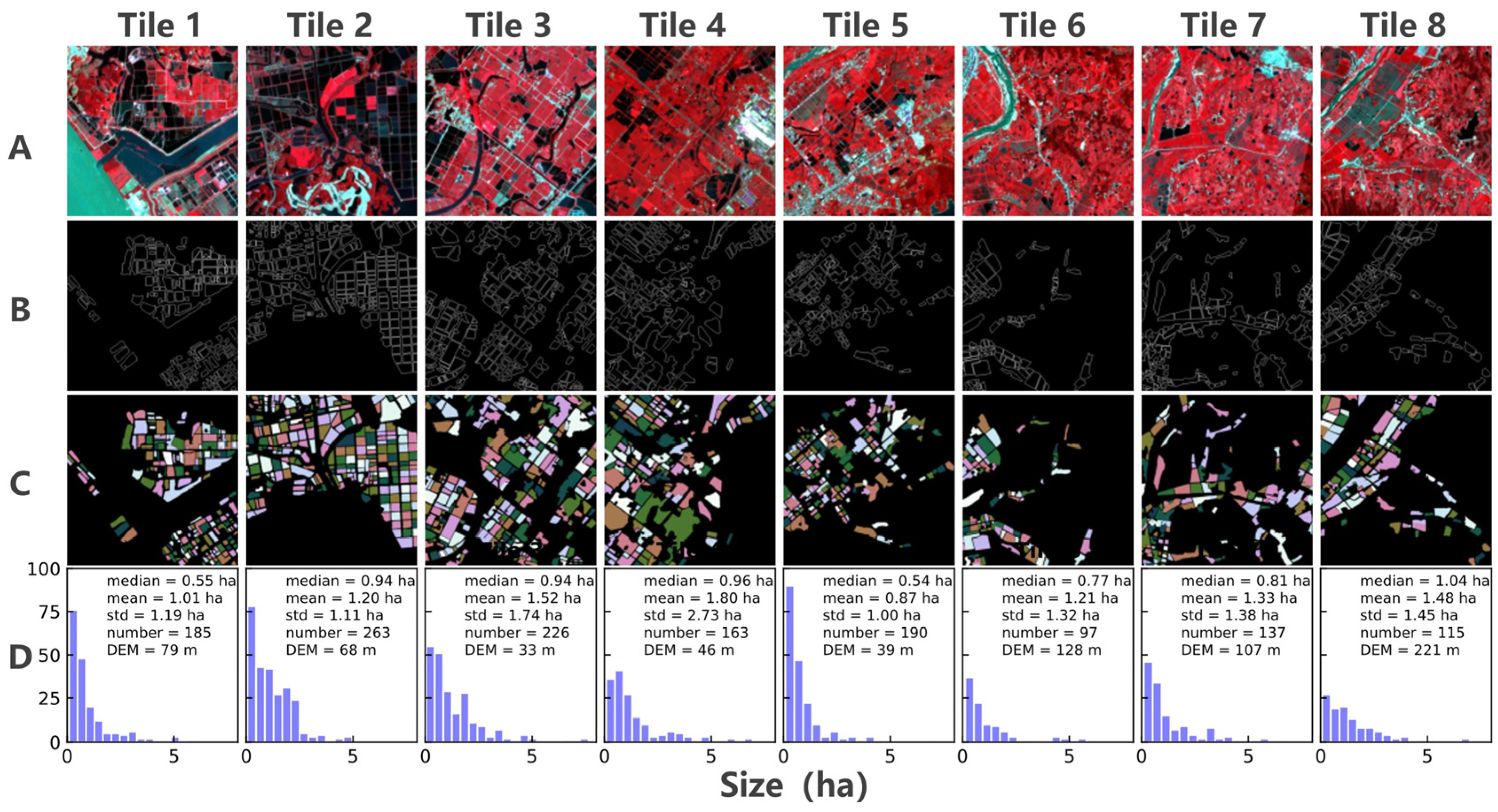
In this study, eight typical test tiles of 3 × 3 km2 areas with different agricultural landscapes were selected, as shown in Figure 1. It can be observed that most cropland parcels were smaller than 2 ha (Figure S1 in Supplementary Materials), suggesting that these tiles can be employed to comprehensively evaluate the performances of cropland parcels derived from MSAOS image segmentation and random forest classification. According to topographic variation and geometric characteristics of cropland parcels (i.e., their sizes and shapes) in Figure 2D, the eight test tiles were grouped into three typical agricultural landscapes, i.e., plain areas with large cropland parcels (PL, i.e., Tiles 2–4), plain areas with small cropland parcels (PS, i.e., Tile 1 and Tile 5), and hilly areas with irregularly shaped cropland parcels (HIS, i.e., Tiles 6–8). Furthermore, cropland parcels in each tile were visually identified by three interpreters using the corresponding Planet images, which were used as the reference cropland parcels to assess the accuracies of extracted cropland parcels.

2.4. Data for Transferability Evaluation

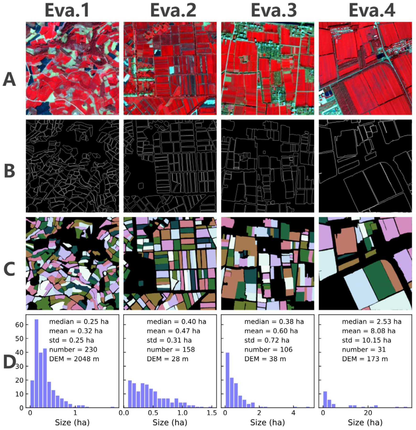
Four typical evaluation tiles (Eva.1–4) of 1 × 1 km2 areas across China from south to north were selected (Figure 1A) to understand the transferability of the MSAOS. Figure 3 demonstrates the shape and size of cropland parcels in these tiles. Eva.1 exhibited the smallest and most irregularly shaped cropland parcels with a median size of 0.25 ha and the largest parcels of smaller than 1.5 ha. Although Eva.2 also displayed the small cropland parcels with a median size of 0.40 ha, it is located on the plain areas and its’ cropland parcels were much more regular. In terms of Eva.3, it showed relatively larger cropland parcels than Eva.2. The largest cropland parcel of Eva.4 was observed due to the high agricultural intensification in the northern China. Overall, the four validation tiles were stratified by the parcel size and included multi landscapes, which could be applied for assessing the MSAOS transferability. Meanwhile, the cropland parcels in each tile were visually interpreted using the corresponding GF-2 images, which were used as the reference data to assess the accuracies of extracted cropland parcels.

3. Methodology

3.1. Calculation of Texture Features

Texture information of high spatial resolution images depicts the correlation between the neighbor pixels, which could reduce the “salt and pepper noise” influence and thus improve the segmentation performance. The gray level cooccurrence matrix (GLCM) method, for which texture information was described via gray-level spatial correlation [34], was used to derive the texture features in this study. The GLCM was calculated with a process window size of 3 × 3 pixels and a cooccurrence shift of (1,1) to extract spatial information from the satellite images (Part 4 in Supplementary Materials). Since there are no guidelines on which texture features are optimal for image segmentation, we calculated candidate texture features from GLCM (Table 1). Then, the optimized texture features for MSAOS were selected by analyzing the separability between cropland and non-cropland in Section 4.1.
Considering the negative impacts of atmospheric scattering on the blue band and the importance of the near-infrared band for vegetation identification, we created an RGB image composition using near-infrared, red, and green bands. Furthermore, to reduce the effect of pseudo boundaries caused by internal color variabilities within the cropland parcels, we used texture information extracted from image luminance instead of chrominance information. Thus, the color space of images was converted from RGB to YUV, in which luminance information was stored in the Y layer and chrominance information was stored in the U and V layers. Subsequently, the candidate texture features were extracted from the Y layer. Finally, we investigated the separability between cropland and non-cropland texture features to select the optimal texture features for obtaining potential cropland objects. Here, we used the separability index to characterize the separability between classes [35], which was calculated using Equation (1):
S I i j = | μ ¯ i μ ¯ j | 1.96 × ( σ i + σ j )
where μ ¯ i ( σ i ) and μ ¯ i ( σ j ) represent the mean (standard deviations) value of class i and class j features, respectively, | μ ¯ i μ ¯ j | denotes the interclass variability, and the ( σ i + σ j ) represents the intraclass variability. Thus, a larger | μ ¯ i μ ¯ j | value and a smaller ( σ i + σ j ) value indicate a higher degree of feature separability between the two classes.

3.2. Image Segmentation by MSAOS

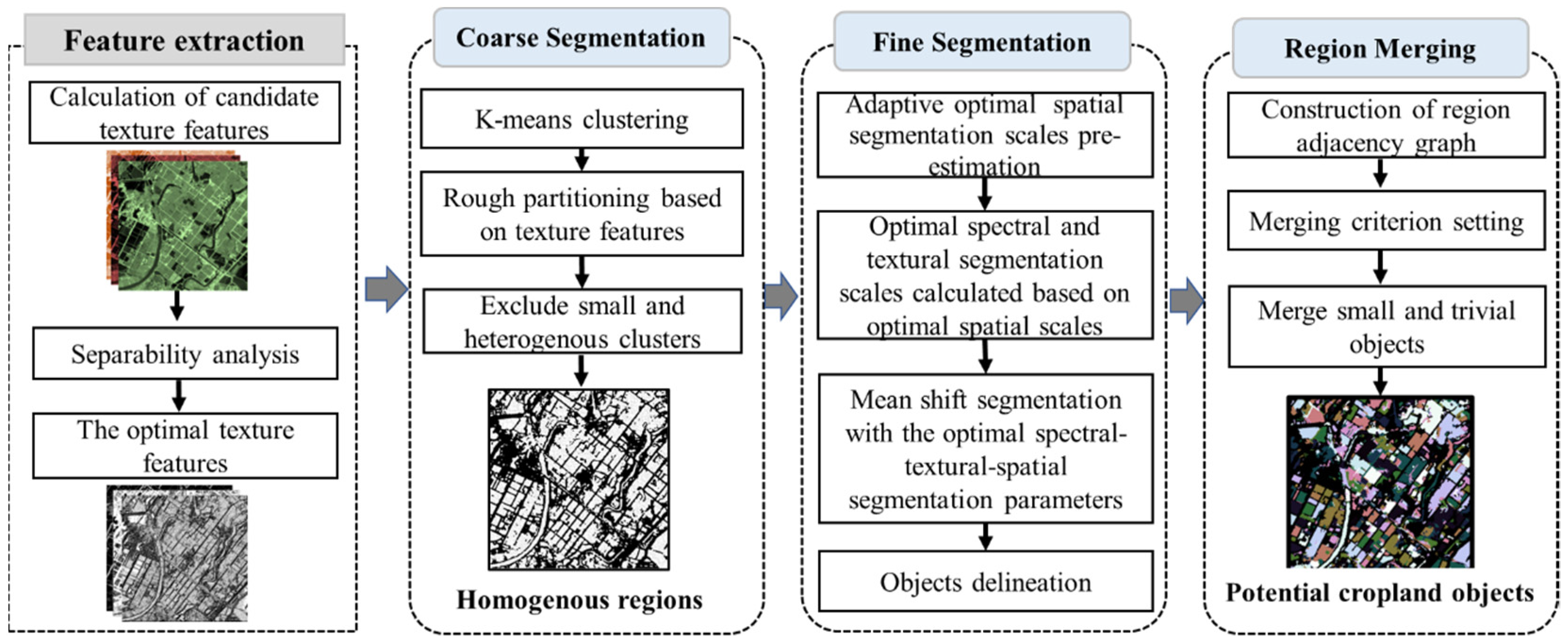
Mean shift is a nonparametric clustering algorithm that uses the Parzen window kernel density estimation to cluster data and has been proven to be effective in image segmentation applications [30,36,37]. The kernel bandwidth (h) is the key parameter for mean shift method, which determines the distance between different clusters in the spatial–spectral–textural domain. This parameter can be further divided into the spatial bandwidth (hs), spectral bandwidth (hr), and texture bandwidth (ht). Specifically, the hs determines the spatial distance between different clusters, while hr and ht limit clusters’ spectral difference and textural difference in the spectral sub-domain and texture sub-domain, respectively. Since an inappropriate h value may result in under- or over-segmentation, this parameter needs to be adaptively adjusted for different landscape types. Here, we developed MSAOS method by extending the traditional mean shift algorithm to automatically select the optimal segmentation scale (Figure 4). Specifically, MSAOS includes three components: (1) First, coarse segmentation was used to divide the whole images into homogenous and heterogeneous regions using k-means clustering based on optimal texture features. (2) Then, for homogenous regions, fine segmentation was conducted to determine the optimal segmentation scale for potential cropland parcels based on average local variance (ALV) functions. (3) Finally, the region-merging algorithm was adopted to merge and dissolve the over-segmented objects with small areas. With the MSAOS method, the potential cropland parcels with their respective optimal cropland boundary were generated.

3.2.1. Coarse Segmentation

The objective of coarse segmentation was to improve the scale estimation of fine segmentation and exclude the heterogeneous objects which were not easily distinguished from croplands by colors. Due to the complexity of landscapes in smallholder farming systems, pre-estimating the optimal kernel bandwidth h for mean shift segmentation based on the whole image information was not necessarily appropriate. This was primarily because the pre-estimated h values obtained for all kinds of objects may ignore the specific characteristics of the targeted objects [23]. For regions with high landscape fragmentation, smaller h values would be more suitable for segmenting small objects, whereas larger h values would be suitable for segmenting larger objects.
To obtain the optimal h for different landscapes, we first divided the whole images into homogenous and heterogeneous regions using the clustering method based on optimal texture features selected in Section 3.1. In this study, the k-means clustering was selected due to its computational efficiency and good performance for segmentation, and the cluster numbers were set as 2, according to the Part 3 in Supplementary Materials. As a result, small objects (e.g., buildings and roads, etc.) or sparse woodlands were characterized by rapidly varying spectra at small spatial scales and thus were assigned to heterogeneous regions. Conversely, larger objects (e.g., cropland parcels, rivers, and large forests) were assigned as homogeneous regions. Thus, the heterogeneous regions were first excluded to reduce the uncertainty in the pre-estimated segmentation scale, and the homogenous regions were retained to pre-estimate the optimal h values for segmenting the cropland parcels.

3.2.2. Fine Segmentation

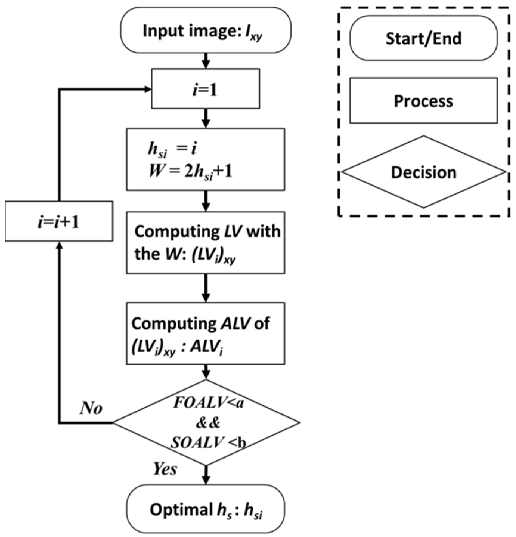
We extended the scale selection method presented by [33] to multilayer images to pre-estimate the optimal h value in the spatial–spectral–textural domain, i.e., hs, hr, and ht, respectively. Figure 5 shows the workflow by which the optimal hs value was pre-estimated.
According to previous studies [32], the relationship between hs and the window size (W) can be expressed as Equation (2):
W = 2 × h s + 1
The optimal hs can be evaluated by iteratively increasing the W values to where the local variance of homogeneous regions converges. First, the local variance (LV) of each pixel was calculated using all pixels within the W × W window size. Particularly, for the LV calculation of border pixels, the symmetric padding method was used to pad the missing pixels outside the region with symmetric pixels along the border. Meanwhile, the ALV of all pixels’ homogeneous regions was calculated. Then, the first-order (FOALV) and the second-order (SOALV) rates of change in ALV were calculated for each iteration, as shown in Equations (3) and (4):
F O A L V i = A L V i A L V i 1 A L V i
S O A L V i = F O A L V i 1 F O A L V i
where i and i − 1 represent the current and previous iteration numbers, respectively; F O A L V i denotes the rate of change in ALV at the i-th iteration; and S O A L V i denotes the change in F O A L V i . Both FOALV and SOALV were employed to assess the dynamics of ALV as the iteration number progresses and their values ranged from 0 to 1. If FOALV and SOALV were both less than the set thresholds of a and b, the current iteration number corresponding hsi was adopted as the optimal hs value. In this study, a and b were set as 0.1 and 0.01, respectively, because these empirically driven thresholds based on the characteristics of study area can maximized the segmentation performance (Part 5 in Supplementary Materials).
Based on the selected hs value, the hr and ht values can be further calculated as the average local standard deviations of the spectral layer and texture layer within the W, respectively, as shown in Equation (5).
h = j = 1 n L V j n
where L V j represent the local variance in the j-th pixel within the W derived by the optimal hs value over the spectral layer or the texture layer. The term n denotes the number of pixels comprised in all homogenous regions.

3.2.3. Region Merging

As a typical bottom-up algorithm, the mean shift method was used to segment the images at pixel level, which could inevitably generate many desired small and trivial segments [38]. For this study, we conducted a region-merging process to address these small segments so as to improve the accuracy of derived cropland parcels. Region merging was a bottom-up process that combines small but similar adjacent regions to obtain a whole large region with certain processing rules. Adjacency judgment and the merging criterion were two prerequisites that need to be carefully addressed in the region-merging process.
In this study, the region adjacency graph (RAG), a data structure widely used to describe the relationship between large-area objects within an image, was employed for the adjacency judgment. The expression of RAG can be defined as G = (V, E), where V was the vertex set that represents regions produced by image segmentation and E was the edge set for the adjacency judgment. In terms of the merging criterion, we used a merging cost function proposed by [38], and this function can be written as Equation (6):
M e r g e ( v i , v j ) = O i × O j ( O i + O j ) × l ( v i , v j ) u i u j 2
where i and j represent the two adjacent regions; O i and O j are the areas of these two regions; u i and u j indicate the feature vectors of regions i and j, respectively; and l ( v i , v j ) denotes the boundary length between two regions. The merging cost function caused the small and trivial segments to be merged with their adjacent regions with larger areas, longer common boundary lengths, and smaller feature differences. Examples of an initial segmentation process, constructed RAG, region-merged RAG, and region-merged segmentation process, are shown in Figure 6. After the initial RAG construction, we conducted a region-merging process based on RAG and merging cost function. Specifically, the merging costs between the target region and its adjacent regions were calculated, and then the target region was merged with one of its adjacent regions by selecting the minimum merge cost. For instance, if region 2 in Figure 6A needed to be merged and the derived M e r g e ( v i , v j ) was minimized based on the calculation of the merge costs between region 2 and its adjacent regions, region 1 and region 2 would be merged to obtain a new region with the label of 1. Then, the RAG was reconstructed subsequently for the next region-merging process until all objects satisfy the region-merging criteria.

3.3. Cropland Identification by Random Forest

We performed a random forest classification to identify cropland parcels from the segmented objects derived by MSAOS. As a typical ensemble learning algorithm, random forest has been demonstrated to be very suited for object-based classification applications in agricultural areas [39]. The random forest classifier used the bagging approach to create a forest consisting of sufficient independent decision trees based on the training set [40]. Each decision tree in the forest makes a determination about the unclassified sample, and each output classification result was obtained as a majority vote of outputs [41]. There were two important parameters for random forest: the number of desired trees (ntree) and the number of features used in each node to make the trees grow (mtry). According to previous classification studies based on random forest [42,43], ntree and mtry were empirically set to 500 and the square root of the total number of input features, respectively.
For our work, three widely-used vegetation indices and seven geometric features were selected as classification features for random forest (Table 2). To adequately characterize the unique phenological characteristics of cropland, these selected spectral and geometric features involving six time points were used as the final features for random forest to identify the croplands parcels.

3.4. Performance Evaluations

We used area- and object-based evaluation methods to fully assess the performances of cropland parcel derived by MSAOS image segmentation and RF classification based on the benchmark cropland dataset. The area-based cropland classification accuracy was assessed using three indicators, i.e., the precision (Pab), recall (Rab), and F1-score (Fab). The Pab measures the proportion of accurately extracted cropland pixels, whereas Rab stands for the proportion of reference cropland pixels that were correctly detected. The F1-score, which combines the precision and recall by calculating the harmonic mean of their values, was used to evaluate the overall accuracy. The three indicators can be calculated as the following Equations (7)–(9):
P ab = T P T P + F P
R ab = T P T P + F N
F ab = 2 × P ab × R ab P ab + R ab
where TP, FP, and FN indicate the number of true positives (pixels correctly identified as cropland), false positives (pixels misclassified as cropland), and false negatives (pixels misclassified as non-cropland), respectively.
In addition, an object-based evaluation method was adopted to understand the source of image segmentation errors, i.e., over- and under-segmentation [44]. The following three indicators, which were implemented based on objects overlapping, can be written as Equations (10)–(12):
P ob = i = 1 n | S i R i m a x | i = 1 n | S i |
R ob = i = 1 m | R i S i m a x | i = 1 m | R i |
F ob = 2 × P ob × R ob P ob + R ob
where S and R represent the segmentation result S with n segments { S 1 , S 2 , S n } and reference results R with m objects { R 1 , R 2 , R m } ; R i m a x and S i m a x were the corresponding reference object and segment with the largest overlapping areas, i.e., S i and R i , respectively; and | R i | denotes the area of Ri. A large precision value (Pob) and a small recall value (Rob) indicate more severe over-segmentation errors, whereas a large Rob and a small Pob denote under-segmentation errors. Fob exhibits the overall segmentation quality by combining Pob and Rob.

4. Results

4.1. The Optimal Texture Features Selected for MSAOS

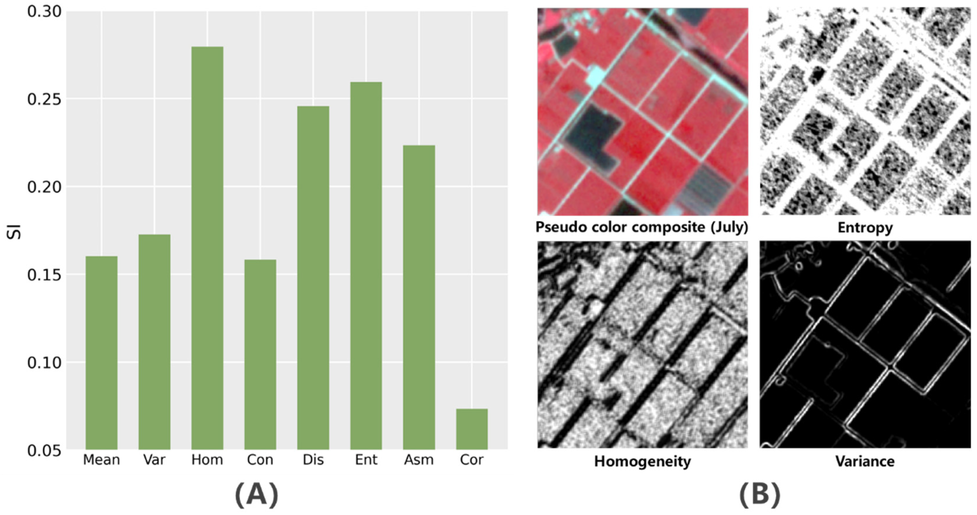
Based on the Planet images in July when crops grow most vigorously in this area, we extracted candidate texture features and analyzed their separability to determine the optimal texture features used for MSAOS. Figure 7A showed the separability index of each candidate texture feature. Features Homogeneity and Entropy exhibited the highest separability between croplands and non-cropland objects, indicating these texture features were most important for obtaining cropland objects. Meanwhile, although Dissimilarity and Angular second moment also showed high separability, they were discarded because of the high correlations with Homogeneity and Entropy (Figure S4 in Supplementary Materials). Features Variance and Contrast also responded to high separability index, which could be because they can reflect the local contrasts within images and helped delineating objects’ boundaries. Since Contrast was easily affected by internal variabilities and pseudo edges, the Variance remained as the input texture feature for MSAOS. An example that shows the maps of optimal texture features was shown in Figure 7B. We found the three features strengthened the edge differentiation between cropland and non-cropland objects. This indicates the usefulness of combining diverse texture features across different observation periods to improve the completeness and precision of cropland parcel extraction in the regions of fragmented agricultural landscapes.

4.2. Maps of Extracted Cropland Parcels

Figure 8 illustrates the cropland parcel extraction results of eight selected tiles at different segmentation steps, including coarse segmentation by k-means clustering, fine segmentation with the optimal segmentation scale and region merging, random forest classification, and the final cropland parcel extraction results. Row B shows that a lot of non-croplands with quite irregular shapes were removed by the coarse segmentation, while a majority of potential cropland objects remained in the coarse segmentation process. However, due to the impacts of inherently high landscape fragmentation, the k-means clustering generated discrete boundaries with under-segmented objects. Based on the coarse segmentation results, fine segmentation was further implemented on the homogenous regions, and individual objects with more precise boundaries were generated (Figure 8C). Moreover, Figure 8C shows cropland objects were more regularly shaped than non-cropland, as expected. Row D displays the object-based classification results, from which we can observe that a variety of cropland parcels in the diverse landscape types were well identified. Since the boundaries among cropland parcels were too narrow to be shown clearly in row D, the boundaries and extents of the individual extracted cropland parcels were further illustrated in rows E and F, respectively.

4.3. Accuracy Assessment of Extracted Cropland Parcels

Table 3 shows the mapping accuracies of cropland parcels for eight test tiles using area- and object-based evaluation methods. Overall, the proposed MSAOS image segmentation combined with random forest classification achieved satisfactory results for cropland parcels, with average Fab and Fob of 0.839 and 0.779, respectively. Specifically, the mapping accuracy was highly related to the landscape fragmentations. The PL group showed the highest accuracy with the average Fab and Fob of 0.872 and 0.829, respectively, followed by the HIS and PS groups. These results indicated that the size of cropland parcels might be the most important factor for the accuracy of cropland parcels extraction, which can be explained by the smallest cropland parcels of PS group in Figure 2D. Nevertheless, the relationship between geometric characteristics and the accuracy of cropland parcels extraction should be further analyzed with the quantitative metrics. Furthermore, it can also be observed that the recall and the precision of the area- (i.e., Rab and Pab) and object-based (i.e., Rob and Pob) evaluations were similar over almost all test tiles, indicating the good capability of the proposed MSAOS method for balancing over- and under-segmentation errors.
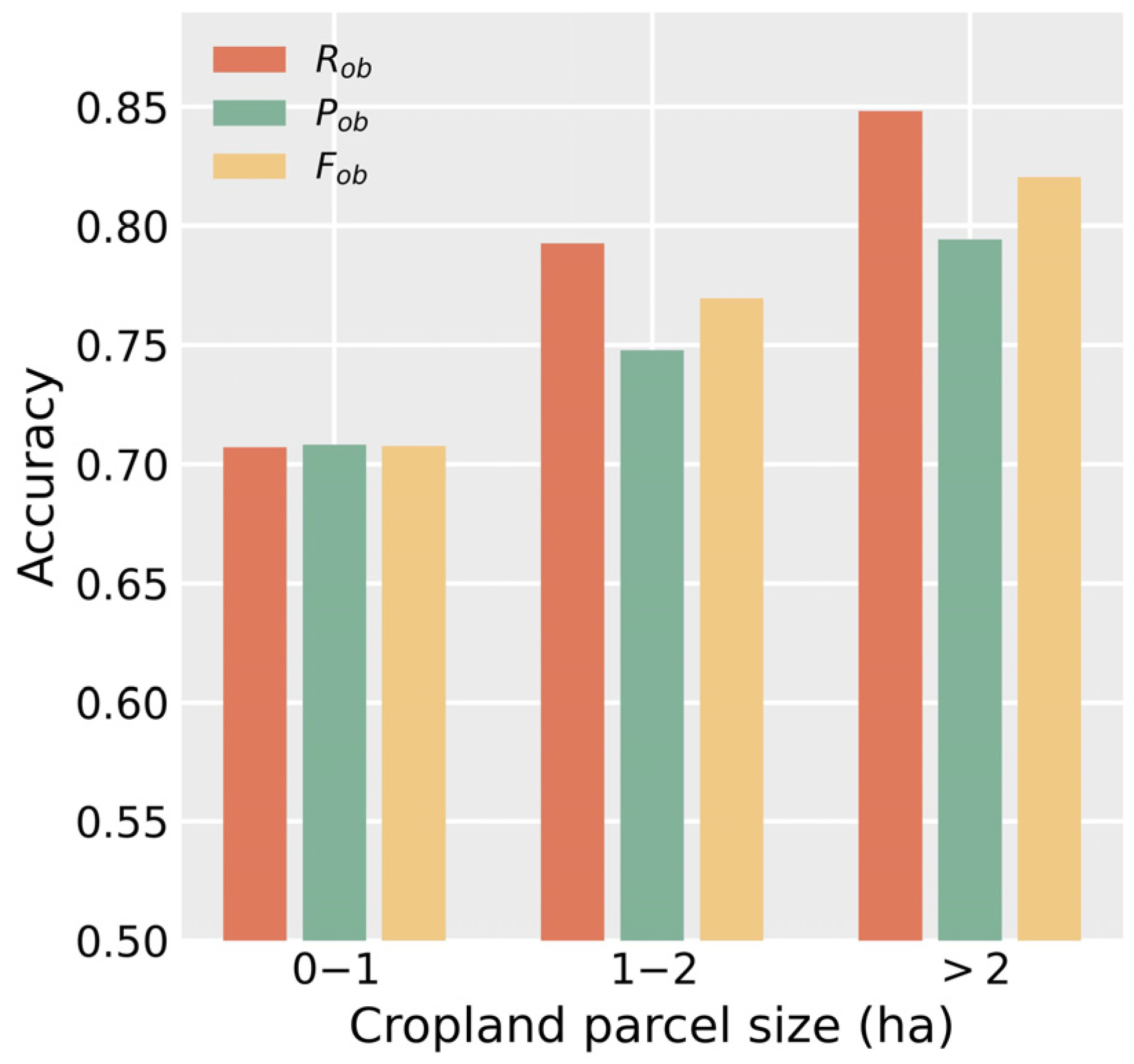
Moreover, the stratified evaluation was implemented to further analyze the performance of the MSAOS in cropland parcels with different sizes (i.e., 0–1 ha, 1–2 ha, and >2 ha) over eight tiles, as shown in Figure 9. Due to the small cropland parcel usually characterized by the narrow and indistinct boundaries, the extraction accuracy of small cropland parcels was lower than that of large cropland parcels as expected. Therefore, the accuracy of smaller cropland parcel (i.e., <1 ha) extraction needs to be further improved in future studies. Overall, these results were consistent with previous studies that indicated the higher landscape fragmentation, and more irregular shaped small cropland parcels could introduce more uncertainties to cropland parcel mapping accuracy.

4.4. Evaluating the Transferability of MSAOS to Other Regions

Table 4 presents the segmentation accuracy for four tiles using the object-based evaluation method. Overall, MSAOS showed similar performance (average Fob of 0.775) to the evaluation results in Section 4.3 (average Fob of 0.779), indicating the good transferability of MSAOS method over different regions. Nevertheless, the MSAOS performance was highly related to cropland parcel size. For regions with large parcels (e.g., Eva.4), MSAOS obtained the highest accuracy with the Fob of 0.878. By contrast, Eva.1–3 with relatively smaller parcels performed worse with the decreasing of Fob by 0.197, 0.127, and 0.090, respectively. Moreover, the better performance of Eva. 2–3 than Eva. 1 also indicated that the cropland with regular shapes can improve the accuracy of cropland parcel extraction.
Additionally, the area-based evaluation method was also implemented to under-stand the commission and omission errors of cropland identification. Overall, the measurement accuracy was consistent with the size and shape of cropland parcels. Eva.4, with the largest regular cropland parcels, obtained the highest Fab of 0.956, whereas Eva.1 derived the worst results due to the small and irregularly shaped cropland parcels. Specifically, the low Fab was mainly caused by the omission error denoted by the low Rab, which can be further explained by the exclusion of heterogeneous regions in coarse segmentation stage. As for regions with small and fragmented agricultural landscapes (e.g., Eva.1), the cropland may be grouped into heterogeneous regions that would be not used in the fine segmentation to extract the cropland parcels. Therefore, the cropland identification in the heterogeneous regions for small and fragmented agricultural landscapes need to be further explored to reduce the misclassification errors.

5. Discussion

5.1. Sensitivity of the Temporal Information Used for Cropland Parcels Extractions

Due to the narrow swath widths and long revisit cycles, high-resolution sensors onboard satellites may have difficulty in obtaining sufficient multi-temporal images over large areas. Thus, it is essential to investigate the sensitivity of temporal information to the performances of cropland identification [20,45,46]. Specifically, we performed two additional classification experiments for MSAOS-derived image objects based on different single-date observations, which were acquired during the growing season (i.e., on 29 July) and nongrowing season (i.e., on 11 October), respectively. The cropland parcel maps obtained for these two single dates and the aforementioned multi-temporal images were assessed by the same validation data.
Table 5 illustrates the cropland parcels extraction results obtained using multi-temporal and single-date images, respectively. The cropland parcels’ accuracy that was assessed by area-based indicators was largely influenced by the crop growth stage. Compared to the classification with single-date information collected in the nongrowing season (SDN), the single-date information collected in the growing season (SDG) provided more useful information for discriminating between croplands and non-croplands, and thus improved the mapping accuracy with average Rab, Pab, and Fab values increased by 0.157, 0.205, and 0.183, respectively. Moreover, the classification based on the multi-temporal images outperformed the two single-date cases, as expected (Rab = 0.833, Pab = 0.846, and Fab = 0.839). Nevertheless, the classification accuracy changed with different agricultural landscapes. For PL regions with large and regular croplands, the SDG-based classification showed a similar accuracy to the multi-temporal-based classification. By contrast, the other two regions (i.e., PS and HIS) that involved multi-temporal information for classification exhibited significant improvement based on three evaluation metrics. In particular, since the cropland parcels were large and crop spectral characteristics in July were different from those of the forest areas within Tile 8, the SDG-based crop identification method also achieved good performance (Fab = 0.854).

5.2. Comparison with Multi-Resolution Segmentation

To further investigate the performance of MSAOS, we compared the cropland parcels derived by MSAOS with that of multi-resolution (MR) segmentation algorithm [20,47]. The reason why we selected the MR segmentation algorithm can be explained from two perspectives. On the one hand, the MR is one of the most popular methods in image segmentation, which has been widely adopted by previous studies [34,48,49]. On the other hand, the MR was also developed based on the bottom-up strategy that is similar to MSAOS method [50]. The scale parameter in the MR algorithm was a prerequisite for achieving good performance for cropland parcel extraction. In this study, five candidate scale parameters (100, 120, 145, 165, and 190) were selected based on the Estimation of Scale Parameter (ESP) tool and visual assessments in eCognition Developer 9.0.2 software [51] so as to obtain the optimal scale parameter value and analyze the relationship between mapping accuracies and segmentation scales (Part 2 in Supplementary Materials). The other segmentation parameters of the MR algorithm, i.e., shape weight and compactness weight, were empirically set as the default values of 0.1 and 0.5, respectively. Similar to MSAOS, a random forest model was used to identify the final cropland parcels from the segmentation results derived using the MR method.
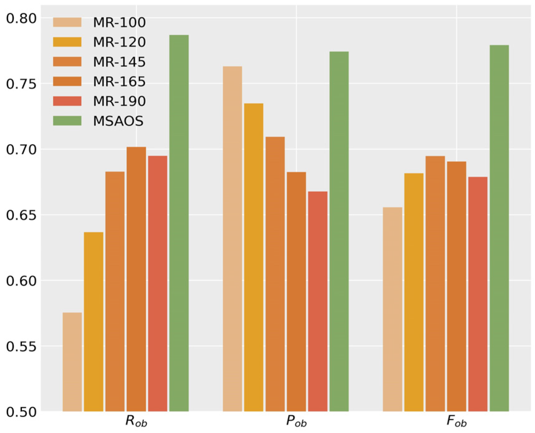
Figure 10 shows the average mapping accuracy of cropland parcels obtained with MSAOS and MR for the eight test tiles, which were both assessed by the segment-based indicators. Overall, the MSAOS method significantly outperformed all MRs with different segmentation scales, showing the highest Rob, Pob, and Fob values among all groups. Although minor changes were observed in the Fob values obtained for MR with different segmentation scales, the major sources of segmentation errors from different MR were distinct. Specifically, the MR algorithm with a segmentation scale of 100 had the highest Pob but the lowest Rob, indicating that more severe over-segmentation errors occurred at a small scale. As the segmentation scale increased, the size of MR-derived segments became bigger, leading to smaller over-segmentation errors (an increased Rob value) but larger under-segmentation errors (a decreased Pob value). Compared with the large variations in MR-derived mapping accuracy, the more stable and better performance of MSAOS indicated that it can provide a good tradeoff between over- and under-segmentation errors.
In detail, Figure 11 displays two representative examples of typical segmentation errors resulting from MR method for Tile 8. For the cropland parcel extraction in example A, MR produced over-segmented results at small scales (e.g., at segmentation scale of 100, 120, and 145) but well-segmented at a larger scale (e.g., segmentation scale of 165 or 190). Furthermore, cropland parcels in example B were well-segmented at small scales (e.g., segmentation scale of 100 and 120) but under-segmented at larger scales (e.g., segmentation scale of 145, 165, and 190). These two examples indicated that the MR method was inferior in obtaining good segmentation results for all cropland parcels at a fixed scale. In contrast, the proposed MSAOS method, which automatically pre-estimated the optimal scale with a two-stage segmentation strategy, could adaptively generate complete and correct cropland parcels, presenting higher robustness for mapping cropland parcels with diverse agriculture landscapes. For instance, the better performance of MSAOS than MR-145, MR-165, and MR-190 for cropland parcel extraction can greatly benefit from the coarse segmentation that assigned the road as heterogeneous region. Thus, the MSAOS was not only helpful for estimating the optimal segmentation scales but also identified the heterogeneous boundaries that cannot be easily recognized by MR methods.

5.3. Strengths and Potential Improvements

High landscape fragmentation with small and irregularly shaped cropland parcels commonly exists in smallholder farming systems, making it challenging for accurate image segmentation based on traditional methods with fixed segmentation scales in such areas. This paper developed an MSAOS method to efficiently extract cropland parcels using high spatial resolution images. Compared to other similar studies [24,34,48], the MSAOS method can automatically pre-estimate the optimal scale to adapt to diverse landscapes with a three-stage segmentation strategy, which significantly improved the accuracy of cropland parcel extraction. Accuracy assessment results indicated that MSAOS provided a good tradeoff between over- and under-segmentation and can largely reduce uncertainties, particularly in regions with fragmented landscapes. Moreover, the experiments of evaluating transferability across spaces (Section 4.4) indicated that the MSAOS can be suitable for extracting cropland parcels in other regions with complex landscapes. Additionally, the computational efficiency of cropland parcel extraction can greatly benefit from the coarse segmentation and the optimal scale selection that were ingested by the MSAOS method (Table S1 in Supplementary Materials).
However, several limitations of MSAOS method should be considered in future studies. First, we performed MSAOS image segmentation using only single-date imagery. As different land surface types might have similar spectral characteristics on a single observation dates, it could result in indistinct boundaries among various land surface types on that specific date and thus add difficulty to cropland parcel segmentation [52]. However, the traditional high-resolution satellites were limited to obtaining VHR images with multiple dates by their narrow swath widths and long revisit cycles [24]. Thus, we only adopted single-date imagery to illustrate the robustness of the MSAOS over different regions. With the rapidly launching high spatial resolution sensors onboard many satellites, the integration of these for obtaining multi-temporal images throughout the crop growing season could be utilized not only for cropland identification (Section 5.1) but also for MSAOS segmentation in the future. Second, although the coarse segmentation was widely implemented using the unsupervised clustering method (i.e., k-means clustering) in which the original images were partitioned based on the differences inherent to the images themselves, this approach might be insufficient for partitioning images containing high landscape fragmentation (e.g., Eva.1 in Section 4.4). In contrast, the application of supervised methods along with training samples may be advantageous to generate more accurate partitions and improve the optimal pre-estimation of the fine segmentation scale [53]. Finally, several studies recently suggested that the combination of edge-based (such as canny operator) and region-based segmentation can detect more accurate boundaries [54], and the proposed MSAOS method could be integrated with edge-based approach to improve the accuracy of delineating cropland parcel boundaries.

6. Conclusions

The irregularly shaped cropland parcels and high landscape fragmentation associated with smallholder farming systems introduce the challenges for extracting cropland parcels in practice. This study developed a new MSAOS method for image segmentation, which was adapted from the mean shift algorithm and implemented the automated selection of the optimal segmentation scale. MSAOS includes three components: (1) First, coarse segmentation was used to divide the whole images into homogenous and heterogeneous regions using k-means clustering based on optimal texture features; (2) then, for homogenous regions, fine segmentation was conducted to determine the optimal segmentation scale for potential croplands parcels based on average local variance (ALV) functions; and (3) finally, the region-merging algorithm was used to merge and dissolve the over-segmented objects with small areas.
Huanggang City of Hubei Province, China, where the agricultural landscape is fragmented and crop planting patterns are complex, was selected as the test area. With MSAOS-derived potential cropland objects, a random forest classification was used to identify the final cropland parcels. The extracted cropland parcels were assessed using digitized benchmark datasets. The results showed that the MSAOS method performed well for extracting cropland parcels, with an average Fab of 0.839 and Fob of 0.779 over eight different landscapes. Compared to the widely used multi-resolution segmentation algorithm, MSAOS provided a better tradeoff between over- and under-segmentation and simultaneously achieved higher average Rob and Pob values of 0.787 and 0.774, respectively. Four evaluation tiles in different provinces were then employed to understand the spatial transferability of the MSAOS method, and the similar results with the average Fab of 0.857 and Fob of 0.775 obtained in transferability evaluation suggested the good performance of the MSAOS over different agricultural regions. Furthermore, texture features Homogeneity and Entropy were the most important features for MSAOS to extract potential cropland parcels, with the highest separability index of 0.286 and 0.272, respectively. Moreover, the use of multi-temporal images was significantly superior to single images in separating cropland and other classes. Overall, the MSAOS method was advantageous for adaptively segmenting cropland parcels of diverse shapes and sizes in complex landscapes, which is promising for mapping cropland parcels in other smallholder farming systems.

Supplementary Materials

The following supporting information can be downloaded at: https://www.mdpi.com/article/10.3390/rs14133067/s1, Figure S1: The distribution of cropland parcel size in 8 test tiles; Figure S2: The candidate scale parameters of multi-resolution segmentation over 8 test tiles using the Estimation of Scale Parameter (ESP) tool; Figure S3: The clustering results of k-means with different clusters numbers; Figure S4: The correlation coefficient between each two texture features; Figure S5: (A) The correlation coefficient between each two co-occurrence shifts, (B) The separability index of Homogeneity feature extracted by different shifts; Figure S6: The relationship between spatial bandwidth and ALV, FOALV and SOALV over the study area; Table S1: The running time of the MSAOS over 8 test tiles.

Author Contributions

Conceptualization, Z.C., Q.H. and B.X.; methodology, Z.C., Q.H., X.Z. and B.X.; software, Z.C.; resources, Q.H. and B.X.; data curation, B.X.; writing—original draft preparation, Z.C.; writing—review and editing, Q.H., X.Z., J.Y., H.W., Z.H., Q.S., G.Y., C.W. and B.X.; visualization, Z.C.; supervision, Q.H. and B.X.; funding acquisition, Q.H. and B.X. All authors have read and agreed to the published version of the manuscript.

Funding

This work was supported by the National Natural Science Foundation of China (42001303, 41901380, 41801371, 41971282), National Key Research and Development Program of China (2019YFE0126700), Young Elite Scientists Sponsorship Program by CAST (2020QNRC001), the Fundamental Research Funds for Central Non-profit Scientific Institution (1610132021010), the Fundamental Research Funds for the Central Universities (2662021JC013, CCNU20QN032), and the Sichuan Science and Technology Program (2021JDJQ0007).

Data Availability Statement

The Planet images and GF-2 images applied in this study can be found at https://www.planet.com/products and http://218.247.138.119:7777/DSSPlatform/productSearch.html, respectively (accessed on 19 June 2022).

Acknowledgments

We sincerely thank the editors and three anonymous reviewers for their detailed and helpful comments which greatly improved this article.

Conflicts of Interest

The authors declare no conflict of interest.

References

  1. Yang, Y.; Huang, Q.; Wu, W.; Luo, J.; Gao, L.; Dong, W.; Wu, T.; Hu, X. Geo-Parcel Based Crop Identification by Integrating High Spatial-Temporal Resolution Imagery from Multi-Source Satellite Data. Remote Sens. 2017, 9, 1298. [Google Scholar] [CrossRef] [Green Version]
  2. Sitokonstantinou, V.; Papoutsis, I.; Kontoes, C.; Arnal, A.; Andrés, A.P.; Zurbano, J.A. Scalable Parcel-Based Crop Identification Scheme Using Sentinel-2 Data Time-Series for the Monitoring of the Common Agricultural Policy. Remote Sens. 2018, 10, 911. [Google Scholar] [CrossRef] [Green Version]
  3. Sun, Y.; Luo, J.; Xia, L.; Wu, T.; Gao, L.; Dong, W.; Hu, X.; Hai, Y. Geo-parcel-based crop classification in very-high-resolution images via hierarchical perception. Int. J. Remote Sens. 2019, 41, 1603–1624. [Google Scholar] [CrossRef]
  4. Dong, W.; Wu, T.; Luo, J.; Sun, Y.; Xia, L. Land parcel-based digital soil mapping of soil nutrient properties in an alluvial-diluvia plain agricultural area in China. Geoderma 2019, 340, 234–248. [Google Scholar] [CrossRef]
  5. Sheng, Y.; Ding, J.; Huang, J. The Relationship between Farm Size and Productivity in Agriculture: Evidence from Maize Production in Northern China. Am. J. Agr. Econ. 2019, 101, 790–806. [Google Scholar] [CrossRef]
  6. Kehoe, L.; Romero-Munoz, A.; Polaina, E.; Estes, L.; Kreft, H.; Kuemmerle, T. Biodiversity at risk under future cropland expansion and intensification. Nat. Ecol. Evol. 2017, 1, 1129–1135. [Google Scholar] [CrossRef]
  7. Rapsomanikis, G. The Economic Lives of Smallholder Farmers: An Analysis Based on Household Data from Nine Countries. Available online: http://www.fao.org/3/a-i5251e.pdf (accessed on 27 January 2022).
  8. Yan, L.; Roy, D.P. Conterminous United States crop field size quantification from multi-temporal Landsat data. Remote Sens. Environ. 2016, 172, 67–86. [Google Scholar] [CrossRef] [Green Version]
  9. Lobell, D.B.; Asner, G.P.; Ortiz-Monasterio, J.I.; Benning, T.L. Remote sensing of regional crop production in the Yaqui Valley, Mexico: Estimates and uncertainties. Agric. Ecosyst. Environ. 2003, 94, 205–220. [Google Scholar] [CrossRef] [Green Version]
  10. Yan, L.; Roy, D.P. Automated crop field extraction from multi-temporal Web Enabled Landsat Data. Remote Sens. Environ. 2014, 144, 42–64. [Google Scholar] [CrossRef] [Green Version]
  11. Graesser, J.; Ramankutty, N. Detection of cropland field parcels from Landsat imagery. Remote Sens. Environ. 2017, 201, 165–180. [Google Scholar] [CrossRef] [Green Version]
  12. Wagner, M.P.; Oppelt, N. Extracting Agricultural Fields from Remote Sensing Imagery Using Graph-Based Growing Contours. Remote Sens. 2020, 12, 1205. [Google Scholar] [CrossRef] [Green Version]
  13. Du, Z.; Yang, J.; Ou, C.; Zhang, T. Smallholder Crop Area Mapped with a Semantic Segmentation Deep Learning Method. Remote Sens. 2019, 11, 888. [Google Scholar] [CrossRef] [Green Version]
  14. Persello, C.; Tolpekin, V.A.; Bergado, J.R.; de By, R.A. Delineation of agricultural fields in smallholder farms from satellite images using fully convolutional networks and combinatorial grouping. Remote Sens. Environ. 2019, 231, 111253. [Google Scholar] [CrossRef] [PubMed]
  15. Zhang, D.; Pan, Y.; Zhang, J.; Hu, T.; Zhao, J.; Li, N.; Chen, Q. A generalized approach based on convolutional neural networks for large area cropland mapping at very high resolution. Remote Sens. Environ. 2020, 247, 111912. [Google Scholar] [CrossRef]
  16. Waldner, F.; Diakogiannis, F.I. Deep learning on edge: Extracting field boundaries from satellite images with a convolutional neural network. Remote Sens. Environ. 2020, 245, 111741. [Google Scholar] [CrossRef]
  17. Wagner, M.P.; Oppelt, N. Deep Learning and Adaptive Graph-Based Growing Contours for Agricultural Field Extraction. Remote Sens. 2020, 12, 1990. [Google Scholar] [CrossRef]
  18. Zhang, H.; Liu, M.; Wang, Y.; Shang, J.; Liu, X.; Li, B.; Song, A.; Li, Q. Automated delineation of agricultural field boundaries from Sentinel-2 images using recurrent residual U-Net. Int. J. Appl. Earth Obs. Geoinf. 2021, 105, 102557. [Google Scholar] [CrossRef]
  19. Ma, L.; Cheng, L.; Li, M.; Liu, Y.; Ma, X. Training set size, scale, and features in Geographic Object-Based Image Analysis of very high resolution unmanned aerial vehicle imagery. ISPRS J. Photogramm. Remote Sens. 2015, 102, 14–27. [Google Scholar] [CrossRef]
  20. Belgiu, M.; Csillik, O. Sentinel-2 cropland mapping using pixel-based and object-based time-weighted dynamic time warping analysis. Remote Sens. Environ. 2018, 204, 509–523. [Google Scholar] [CrossRef]
  21. Johansen, K.; Lopez, O.; Tu, Y.-H.; Li, T.; McCabe, M.F. Center pivot field delineation and mapping: A satellite-driven object-based image analysis approach for national scale accounting. ISPRS J. Photogramm. Remote Sens. 2021, 175, 1–19. [Google Scholar] [CrossRef]
  22. Zhou, W.; Ming, D.; Xu, L.; Bao, H.; Wang, M. Stratified Object-Oriented Image Classification Based on Remote Sensing Image Scene Division. J. Spectrosc. 2018, 2018, 1–11. [Google Scholar] [CrossRef] [Green Version]
  23. Xu, L.; Ming, D.; Zhou, W.; Bao, H.; Chen, Y.; Ling, X. Farmland Extraction from High Spatial Resolution Remote Sensing Images Based on Stratified Scale Pre-Estimation. Remote Sens. 2019, 11, 108. [Google Scholar] [CrossRef] [Green Version]
  24. Cheng, T.; Ji, X.; Yang, G.; Zheng, H.; Ma, J.; Yao, X.; Zhu, Y.; Cao, W. DESTIN: A new method for delineating the boundaries of crop fields by fusing spatial and temporal information from WorldView and Planet satellite imagery. Comput. Electron. Agric. 2020, 178, 105787. [Google Scholar] [CrossRef]
  25. Witharana, C.; Bhuiyan, M.A.E.; Liljedahl, A.K.; Kanevskiy, M.; Jorgenson, T.; Jones, B.M.; Daanen, R.; Epstein, H.E.; Griffin, C.G.; Kent, K.; et al. An Object-Based Approach for Mapping Tundra Ice-Wedge Polygon Troughs from Very High Spatial Resolution Optical Satellite Imagery. Remote Sens. 2021, 13, 558. [Google Scholar] [CrossRef]
  26. Su, T.; Li, H.; Zhang, S.; Li, Y. Image segmentation using mean shift for extracting croplands from high-resolution remote sensing imagery. Remote Sens. Lett. 2015, 6, 952–961. [Google Scholar] [CrossRef]
  27. Li, D.; Zhang, G.; Wu, Z.; Yi, L. An edge embedded marker-based watershed algorithm for high spatial resolution remote sensing image segmentation. IEEE Trans. Image Process. 2010, 19, 2781–2787. [Google Scholar] [CrossRef]
  28. Chen, B.; Qiu, F.; Wu, B.; Du, H.J.R.S. Image segmentation based on constrained spectral variance difference and edge penalty. Remote Sens. 2015, 7, 5980–6004. [Google Scholar] [CrossRef] [Green Version]
  29. Benz, U.C.; Hofmann, P.; Willhauck, G.; Lingenfelder, I.; Heynen, M. Multi-resolution, object-oriented fuzzy analysis of remote sensing data for GIS-ready information. ISPRS J. Photogramm. Remote Sens. 2004, 58, 239–258. [Google Scholar] [CrossRef]
  30. Comaniciu, D.; Meer, P. Mean shift: A robust approach toward feature space analysis. IEEE Trans. Pattern Anal. Mach. Intell. 2002, 24, 603–619. [Google Scholar] [CrossRef] [Green Version]
  31. Huang, X.; Zhang, L. An Adaptive Mean-Shift Analysis Approach for Object Extraction and Classification From Urban Hyperspectral Imagery. IEEE Trans. Geosci. Remote Sens. 2008, 46, 4173–4185. [Google Scholar] [CrossRef]
  32. Ming, D.; Ci, T.; Cai, H.; Li, L.; Qiao, C.; Du, J. Semivariogram-Based Spatial Bandwidth Selection for Remote Sensing Image Segmentation With Mean-Shift Algorithm. IEEE Geosci. Remote Sens. Lett. 2012, 9, 813–817. [Google Scholar] [CrossRef]
  33. Ming, D.; Li, J.; Wang, J.; Zhang, M. Scale parameter selection by spatial statistics for GeOBIA: Using mean-shift based multi-scale segmentation as an example. ISPRS J. Photogramm. Remote Sens. 2015, 106, 28–41. [Google Scholar] [CrossRef]
  34. Lu, H.; Liu, C.; Li, N.; Fu, X.; Li, L. Optimal segmentation scale selection and evaluation of cultivated land objects based on high-resolution remote sensing images with spectral and texture features. Environ. Sci. Pollut. Res. Int. 2021, 28, 27067–27083. [Google Scholar] [CrossRef]
  35. Somers, B.; Asner, G.P. Multi-temporal hyperspectral mixture analysis and feature selection for invasive species mapping in rainforests. Remote Sens. Environ. 2013, 136, 14–27. [Google Scholar] [CrossRef]
  36. Zhou, H.; Li, X.; Schaefer, G.; Celebi, M.E.; Miller, P. Mean shift based gradient vector flow for image segmentation. Comput. Vis. Image Underst. 2013, 117, 1004–1016. [Google Scholar] [CrossRef] [Green Version]
  37. Lang, F.; Yang, J.; Yan, S.; Qin, F. Superpixel Segmentation of Polarimetric Synthetic Aperture Radar (SAR) Images Based on Generalized Mean Shift. Remote Sens. 2018, 10, 1592. [Google Scholar] [CrossRef] [Green Version]
  38. Fu, G.; Zhao, H.; Li, C.; Shi, L. Segmentation for High-Resolution Optical Remote Sensing Imagery Using Improved Quadtree and Region Adjacency Graph Technique. Remote Sens. 2013, 5, 3259–3279. [Google Scholar] [CrossRef] [Green Version]
  39. Li, M.; Ma, L.; Blaschke, T.; Cheng, L.; Tiede, D. A systematic comparison of different object-based classification techniques using high spatial resolution imagery in agricultural environments. Int. J. Appl. Earth Obs. Geoinf. 2016, 49, 87–98. [Google Scholar] [CrossRef]
  40. Immitzer, M.; Vuolo, F.; Atzberger, C. First Experience with Sentinel-2 Data for Crop and Tree Species Classifications in Central Europe. Remote Sens. 2016, 8, 166. [Google Scholar] [CrossRef]
  41. Breiman, L.J.M.l. Random forests. Mach. Learn. 2001, 45, 5–32. [Google Scholar] [CrossRef] [Green Version]
  42. Immitzer, M.; Atzberger, C.; Koukal, T. Tree Species Classification with Random Forest Using Very High Spatial Resolution 8-Band WorldView-2 Satellite Data. Remote Sens. 2012, 4, 2661–2693. [Google Scholar] [CrossRef] [Green Version]
  43. Hu, Q.; Yin, H.; Friedl, M.A.; You, L.; Li, Z.; Tang, H.; Wu, W. Integrating coarse-resolution images and agricultural statistics to generate sub-pixel crop type maps and reconciled area estimates. Remote Sens. Environ. 2021, 258, 112365. [Google Scholar] [CrossRef]
  44. Zhang, X.; Feng, X.; Xiao, P.; He, G.; Zhu, L. Segmentation quality evaluation using region-based precision and recall measures for remote sensing images. ISPRS J. Photogramm. Remote Sens. 2015, 102, 73–84. [Google Scholar] [CrossRef]
  45. Waldner, F.; Canto, G.S.; Defourny, P. Automated annual cropland mapping using knowledge-based temporal features. ISPRS J. Photogramm. Remote Sens. 2015, 110, 1–13. [Google Scholar] [CrossRef]
  46. Xiong, J.; Thenkabail, P.; Tilton, J.; Gumma, M.; Teluguntla, P.; Oliphant, A.; Congalton, R.; Yadav, K.; Gorelick, N. Nominal 30-m Cropland Extent Map of Continental Africa by Integrating Pixel-Based and Object-Based Algorithms Using Sentinel-2 and Landsat-8 Data on Google Earth Engine. Remote Sens. 2017, 9, 1065. [Google Scholar] [CrossRef] [Green Version]
  47. Jozdani, S.E.; Momeni, M.; Johnson, B.A.; Sattari, M. A regression modelling approach for optimizing segmentation scale parameters to extract buildings of different sizes. Int. J. Remote Sens. 2017, 39, 684–703. [Google Scholar] [CrossRef]
  48. Wen, C.; Lu, M.; Bi, Y.; Zhang, S.; Xue, B.; Zhang, M.; Zhou, Q.; Wu, W. An Object-Based Genetic Programming Approach for Cropland Field Extraction. Remote Sens. 2022, 14, 1275. [Google Scholar] [CrossRef]
  49. Shen, Y.; Chen, J.; Xiao, L.; Pan, D. Optimizing multiscale segmentation with local spectral heterogeneity measure for high resolution remote sensing images. ISPRS J. Photogramm. Remote Sens. 2019, 157, 13–25. [Google Scholar] [CrossRef]
  50. Ming, D.; Zhang, X.; Wang, M.; Zhou, W. Cropland Extraction Based on OBIA and Adaptive Scale Pre-estimation. Photogramm. Eng. Remote Sens. 2016, 82, 635–644. [Google Scholar] [CrossRef]
  51. Trimble. eCognition Developer 9.0.1 Reference Book; Trimble Germany GmbH: Munich, Germany, 2014. [Google Scholar]
  52. Watkins, B.; van Niekerk, A. A comparison of object-based image analysis approaches for field boundary delineation using multi-temporal Sentinel-2 imagery. Comput. Electron. Agric. 2019, 158, 294–302. [Google Scholar] [CrossRef]
  53. Xu, L.; Ming, D.; Du, T.; Chen, Y.; Dong, D.; Zhou, C. Delineation of cultivated land parcels based on deep convolutional networks and geographical thematic scene division of remotely sensed images. Comput. Electron. Agric. 2022, 192, 106611. [Google Scholar] [CrossRef]
  54. Watkins, B.; Van Niekerk, A. Automating field boundary delineation with multi-temporal Sentinel-2 imagery. Comput. Electron. Agric. 2019, 167, 106611. [Google Scholar] [CrossRef]
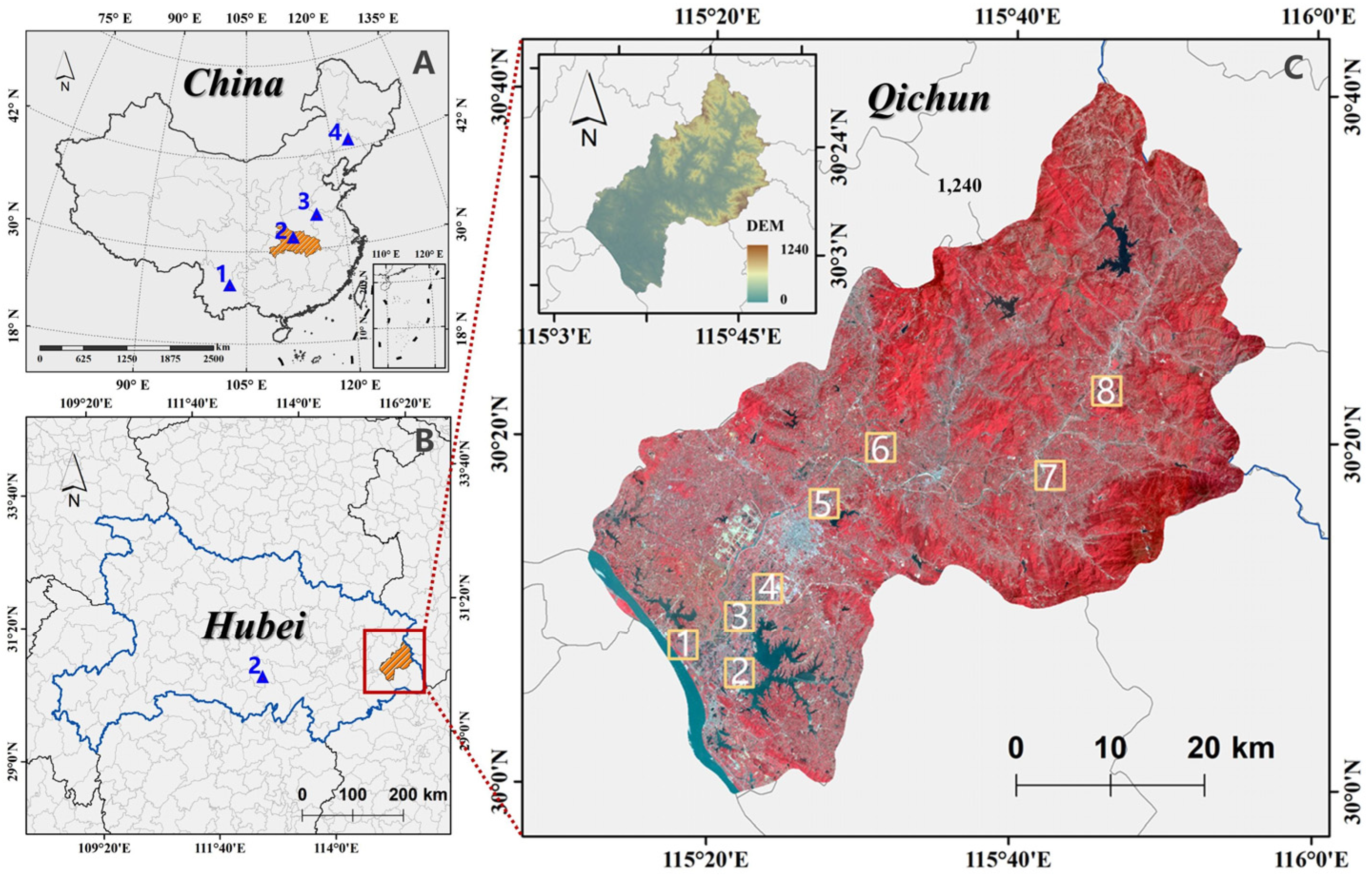
Figure 1. The spatial location of the selected test regions used for the cropland parcel extraction and the other four regions for evaluating the transferability of the MSAOS. (A) is the spatial distribution of the test region (orange area) and the evaluation tiles (four blue triangles); (B) details the geographic location of test region and the evaluation tile in Hubei province; The top-left inset and large pictures in panel (C) refer to a digital elevation map (DEM) and pseudo-color (RGB: near-infrared, red, and green) image of Qichun, respectively. The squares with yellow solid lines in panel (C) are the selected test tiles used to evaluate the MSAOS performance.
Remotesensing 14 03067 g001
Figure 2. The eight typical test tiles and associated reference cropland parcels in this study. (A) The pseudo-color composition image of each tile, (B) boundaries of the reference cropland parcels, (C) individual cropland parcels denoted by random colors, and (D) the cropland parcel size distributions and the topological characteristics over eight typical test tiles.
Remotesensing 14 03067 g002
Figure 3. The four typical evaluation tiles and associated reference cropland parcels in this study. (A) The pseudo-color composition image of each tile, (B) boundaries of the reference cropland parcels, (C) individual cropland parcels denoted by random color, and (D) the cropland parcel size distributions and the topological characteristics over four tiles.
Remotesensing 14 03067 g003
Figure 4. The workflow of extracting potential cropland parcels based on the MSAOS.
Remotesensing 14 03067 g004
Figure 5. The workflow of selecting the optimal hs value for the mean shift algorithm.
Remotesensing 14 03067 g005
Figure 6. Example of the region-merging process: (A) initial segmentation result; (B) RAG of (A); (C) RAG after region merging; (D) region-merging result.
Remotesensing 14 03067 g006
Figure 7. (A) Separability index (SI) values calculated for all texture features; (B) an example of the selected optimal texture features.
Remotesensing 14 03067 g007
Figure 8. Cropland parcel extraction results derived at different processing steps for eight test tiles. (A) Pseudo-color composite imagery of each tile; (B) the coarse segmentation results, with the homogenous regions denoted by the white color; (C) the fine segmentation results, indicated by the use of a random color for each object; (D) the object-based classification results derived using the trained random forest model (the generated croplands are shown with a cyan color); (E) the extracted boundaries (white lines) of the final cropland parcels; and (F) the final cropland parcels denoted by random colors.
Remotesensing 14 03067 g008
Figure 9. Stratified object-based evaluation results based on the size of cropland parcels.
Remotesensing 14 03067 g009
Figure 10. The average Rob, Pob, and Fob values obtained for the eight test tiles using the MSAOS and MR segmentation algorithms with five segmentation scales: 100, 120, 145, 165 and 190.
Remotesensing 14 03067 g010
Figure 11. Detailed comparisons of the cropland parcel extraction results derived by MSAOS and MR methods with different segmentation scales. The numbers (e.g., 100) refer to the segmentation scales of the MR method.
Remotesensing 14 03067 g011
Table 1. Candidate texture features used for image segmentation.
Feature NameEquation
Mean M e a n = 1 L 2 i = 0 L 1 j = 0 L 1 P i j
Variance (Var) V a r = i = 0 L 1 j = 0 L 1 ( i M e a n ) 2 P i j
Homogeneity (Hom) H o m = i = 0 L 1 j = 0 L 1 P i j 1 + ( i j ) 2
Contrast (Con) C o n = i = 0 L 1 j = 0 L 1 ( i j ) 2 P i j
Dissimilarity (Dis) D i s = i = 0 L 1 j = 0 L 1 | i j | P i j
Entropy (Ent) E n t = i = 0 L 1 j = 0 L 1 P i j ( lg ( P i j ) )
Angular second moment (ASM) A S M = i = 0 L 1 j = 0 L 1 P i j 2
Correlation (Cor) C o r = i = 0 L 1 j = 0 L 1 ( i M e a n ) ( j M e a n ) P i j 2 V a r
Both i and j represent the pixel gray level, L indicates the grayscale of the image, and P i j denotes each GLCM element.
Table 2. List of the spectral and geometric features used in this study. The term “i” denotes the specific observation date of the remote sensing image.
Feature TypeFeature NameEquation or Explanation
Spectral featuresNDVI N D V I i = N i r i R i N i r i + R i
VIgreen V I g r e e n i = G i R i G i + R i
EVI E V I i = 2.5 × N i r i R i N i r i + 6 R i 7.5 B i + 1
Geometric featuresAreaThe area of the object.
PerimeterThe perimeter of the object.
ShinThe shape index, computed as perimeter/( 4 A r e a ), the closer the shape index value of the object is to 1, the more regular the object is.
ExtentComputed as the area divided by the area of the smallest rectangle containing the object.
Minor axis lengthLength of the minor axis of the ellipse that has the same normalized second central moment as the object.
Major axis lengthLength of the major axis of the ellipse that has the same normalized second central moment as the object.
OrientationAngle between the x-axis and the major axis of the ellipse that has the same second moment as the object.
Table 3. Evaluation of the area- and object-based accuracy of the cropland parcel extraction results. PS, PL, and HIS indicate three different agricultural landscape types, i.e., plain areas with large cropland parcels, plain areas with small cropland parcels, and hilly areas with irregularly shaped cropland parcels, that were described in Section 2.3.
Evaluation MethodsPSPLHISAVG
Tile 1Tile 5Tile 2Tile 3Tile 4Tile 6Tile 7Tile 8
Area-based evaluationRab0.7860.7950.8340.8640.8860.8060.8130.8810.833
Pab0.7980.8170.9350.8880.8290.8440.8060.8510.846
Fab0.7920.8060.8820.8760.8560.8240.8090.8650.839
Object-based evaluationRob0.720 0.745 0.822 0.853 0.867 0.708 0.753 0.827 0.787
Pob0.749 0.746 0.901 0.829 0.720 0.736 0.714 0.799 0.774
Fob0.734 0.745 0.860 0.841 0.786 0.722 0.7370.8130.779
Table 4. Accuracy assessments of tiles in different provinces.
Evaluation MethodsEva.1Eva.2Eva.3Eva.4AVG
Area-based
evaluation
Pab0.9310.9360.9930.9750.959
Rab0.6660.7110.8030.9380.780
Fab0.7770.8080.8880.9560.857
Object-based
evaluation
Pob0.7930.8720.8890.9720.882
Rob0.5960.6600.7070.8010.691
Fob0.6810.7510.7880.8780.775
Table 5. The area-based accuracy evaluation results obtained using object-based classification with multi-temporal (MT) information, single-date observation in the growing season (SDG) information, and single-date observation in the nongrowing season (SDN) information. “AVG” represents the average value of the eight test tiles. The bold numbers in the table denote the accuracy of the classification strategy adopted in this study.
TileRabPabFab
SDNSDGMTSDNSDGMTSDNSDGMT
PSTile 10.514 0.7250.7860.584 0.7660.7980.547 0.7450.792
Tile 50.521 0.7400.7950.450 0.8010.8170.483 0.7690.806
PLTile 20.693 0.8070.8340.715 0.9120.9350.704 0.8560.882
Tile 30.650 0.8440.8640.780 0.9010.8880.709 0.8720.876
Tile 40.741 0.8750.8860.700 0.8340.8290.720 0.8540.856
HISTile 60.532 0.6610.8060.407 0.7970.8440.461 0.7220.824
Tile 70.601 0.7110.8130.642 0.7370.8060.621 0.7240.809
Tile 80.723 0.8720.8810.666 0.8370.8510.693 0.8540.865
AVG0.622 0.7790.8330.618 0.8230.8460.617 0.8000.839
Publisher’s Note: MDPI stays neutral with regard to jurisdictional claims in published maps and institutional affiliations.