Abstract
The Copernicus high-resolution layer imperviousness density (HRL IMD) for 2018 is a 10 m resolution raster showing the degree of soil sealing across Europe. The imperviousness gradation (0–100%) per pixel is determined by semi-automated classification of remote sensing imagery and based on calibrated NDVI. The product was assessed using a within-pixel point sample of ground truth examined on very high-resolution orthophoto for the section of the product covering Norway. The results show a high overall accuracy, due to the large tracts of natural surfaces correctly portrayed as permeable (0% imperviousness). The total sealed area in Norway is underestimated by approximately 33% by HRL IMD. Point sampling within pixels was found to be suitable for verification of remote sensing products where the measurement is a binomial proportion (e.g., soil sealing or canopy coverage) when high-resolution aerial imagery is available as ground truth. The method is, however, vulnerable to inaccuracies due to geometrical inconsistency, sampling errors and mistaken interpretation of the ground truth. Systematic sampling inside each pixel is easy to work with and is known to produce more accurate estimates than a simple random sample when spatial autocorrelation is present, but this improvement goes unnoticed unless the status and location of each sample point inside the pixel is recorded and an appropriate method is applied to estimate the within-pixel sampling accuracy.
1. Introduction
Population growth and economic development are driving forces behind land use change [1]. A growing population customize their surroundings by replacing natural surfaces with a solid covering consisting of concrete surfaces, buildings, paved roads, and other constructions that create an impervious land cover [2]. This process, known as soil sealing, separates the soils from the atmosphere by one or more impermeable layers [3]. The result is, among other effects, a loss of area available for plant production, reduced biodiversity, and an increase in run-off of surface water [4,5,6]. Soil sealing is therefore considered as an example of land degradation [7] and imperviousness is frequently used as an indicator of land take in environmental monitoring [8].
There has been an increasing interest in mapping soil sealing and imperviousness over the last 30 years [9]. Around the turn of the century, USGS derived a measurement of soil sealing from Landsat imagery for the 2001 National Land Cover database for the United States, using the degree of imperviousness as their indicator [10,11]. In Europe, statistics of sealed surfaces over larger zones were first generated using the SPOT VEGETATION imagery from 2001, with a spatial resolution of 1 km [12]. Better spatial resolution was achieved in 2005, by mapping soil sealing using the normalized difference vegetation index (NDVI) calculated from QuickBird imagery [13].
A systematic comparison of different approaches to measure soil sealing using air photo interpretation showed an average overall agreement between existing products at 92% [14]. A comprehensive review of techniques using medium resolution (10–100 m) imagery was published in 2012, describing trends in remote sensing of impervious surfaces [15]. These include pixelwise estimation of imperviousness degree, classification of surface material or and mapping land cover or land use features (e.g., buildings or roads) in order to infer imperviousness from land cover/use. A variety of new attempts to develop automated methods for detecting soil sealing and measure the degree of imperviousness have later been published, employing new and improved remote sensing imagery and classification techniques [16,17,18]. The most recent review of research on soil sealing, land take and impervious surfaces lists eleven different mapping methods currently in use [19].
The European Union’s Earth observation program, Copernicus, conducts projects to monitor land cover and land use in order to serve urban and environmental planning and policy making. One outcome from this program is the high-resolution layer imperviousness density (HRL IMD). This is a service provided through the Copernicus land monitoring service (CLMS, https://land.copernicus.eu/, last accessed on 7 June 2022) implemented by the European Environment Agency (EEA). HRL IMD is a raster product estimating the degree of imperviousness within each pixel.
The environmental indicator mapped by HRL IMD is defined as “human-produced surfaces that are essentially impenetrable by rainfall” [20]. This is a binary phenomenon since a location on a surface is either sealed or not sealed. When used as an indicator, imperviousness is reported as the proportion of the land surface covered by a pixel that is impenetrable to water and therefore creates increased surface runoff [11,21], leading to a gradation on the scale 0–100%. The variable is a binomial proportion reported as a percentage.
The HRL IMD product covers the entire European continent and has so far been produced for the reference years 2006, 2009, 2012, 2015 and 2018. The 2018 product has 10 m resolution, while the older products have 20 m resolution. The first updates relied on a semi-automated approach (mainly due to the limited availability of input data). The level of automation of the production has steadily increased due to the availability of better reference data and improved resolution of remote sensing imagery [22].
Data from the Copernicus land monitoring service are used, or are proposed to be used, in studies and reports from Eurostat and the European Environmental Agency [23,24]. It is also a goal to serve urban and environmental planning and policy making at the national and local level. Detailed knowledge of the content and accuracy of the product is, however, a prerequisite for the broader user-uptake of the service. Users need to understand the content of the product to interpret and use the data correctly. Verification has been carried out in several countries, often using a qualitative “look and feel” approach [25] and a technical validation of the 2015 version of HRL IMD is also available [26].
A study of the accuracy of the US National Land Cover Data for 2006 found that the ideal accuracy assessment of imperviousness data would require estimation of the impervious surface for each sample pixel from reference data, but the cost to obtain the required data was considered prohibitive [27]. New technology and high-resolution aerial photography have changed this situation and detailed information about the content of pixels can now be used as reference data. The cost of a complete inventory of the pixel using analytical photogrammetry is, however, still exorbitant. Instead, we may attempt a sampling approach by obtaining a random sample of points inside each control pixel.
The objective of the current study was to examine the content and accuracy of the HRL IMD product for 2018 using a within-pixel sampling approach. Norway was used as a study area due to the availability of high-resolution and geometrically accurate orthophoto acquired through an established and regular national image acquisition program. The goal was to examine the potential and limitations of the within-pixel sampling approach to verification, but also to improve the interpretation and understanding of the HRL IMD product and thus enhance the value of the product for the end-users.
2. Materials and Methods
The high-resolution layer imperviousness density (HRL IMD) 2018 for Norway was downloaded from the Copernicus land monitoring service (CLMS) web site https://land.copernicus.eu, accessed on 6 January 2021. The tiles covering Norway were combined to create a raster with national coverage. The projection of the map was ETRS89-LAEA89 (EPSG: 3035, https://epsg.io, last accessed on 7 June 2022). The dataset is a 10 m raster where each pixel is coded in the range 0–100, representing the degree of imperviousness in percent.
Two web map services (wms) were used to obtain ground truth: the Norwegian national topographic maps at scales ranging between 1:1000 and 1:5000 provided by the National Mapping Authority and the national orthophoto database (Norge i bilder) provided by the Norwegian Spatial Data Infrastructure Norge digitalt. Data from these sources have national coverage and could be linked directly to the QGIS software used in the study. The imagery and other data that were used as ground truth can be inspected at https://kilden.nibio.no/, last accessed on 7 June 2022.
A two-stage random sample was collected to examine the accuracy of the HRL IMD layer. Stratification was employed in the first stage because most pixels (99.4%) had no reported imperviousness (0%). Only 0.6% of the pixels had imperviousness density in the range 1 to 100%.
The data were divided into twelve strata according to the reported imperviousness (0%, 1–9%, 10–19% {…} 90–99% and 100%, see also Table 1), providing a basis for stratified random sampling. The two strata “0%” and “100%” represent the extremes. “0%” also constitute a very large part of the population and should therefore be given special attention since a relatively large sample is required to detect small anomalies in large strata. The number and size of the ten remaining strata was a compromise between the need for detail (requiring many strata) and available resources.

Table 1.
Imperviousness in Norway as reported by HRL IMD and as estimated by sampling. The total land area (32,380,900 hectares) is divided into strata according to the degree of imperviousness reported by HRL IMD. Mean imperviousness and the corresponding sealed area were calculated for each stratum, as well as for a subtotal of all strata with reported imperviousness (according to HRL IMD) and for the whole country.
The sampling procedure selected (randomly) 1000 points from the stratum where the reported imperviousness was 0% and attempted to select (randomly) 100 points from each of the remaining strata. The stratum with imperviousness in the range 1 to 9% was, however, so rare that we only managed to find 82 sample points in this stratum. The final, stratified random sample consisted of 2082 sample points. This sample size is pragmatic, mainly linked to available funding and acceptable sampling cost. Various aspects of the sampling strategy are discussed in the Section 4 below.
A sampling tool was developed in Python for QGIS. The tool starts from a sample point in the stratified random sample and locates the corresponding 10 m pixel in HRL IMD. A border is drawn around the pixel and a new, systematic random sample of 100 points is placed inside the pixel. The first point is placed 0.5 m north and 0.5 m east of the lower left corner of the pixel. The remaining points are spaced along a regular lattice, one meter apart, throughout the pixel (Figure 1). The observed imperviousness was calculated by counting the number of points (0–100) that fell on impenetrable surfaces as defined in the HRL IMD technical documentation [28].
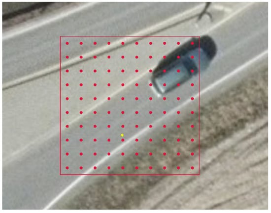
Figure 1.
A 10 m pixel in HRL IMD with 100 sample points (red dots). The yellow dot shows the original random sample point used to detect and include this pixel. Photo obtained during the summer of 2017. Data source: © Norge i bilder/Norge digitalt.
Formally, the population examined using this approach consists of all N pixels in the HRL IMD layer divided into M strata with Ni pixels in each stratum. A simple random sample of ni pixels is drawn from each stratum, resulting in a total sample size of
(where n is 2082). Notice that the sample is not proportional, that is mainly due to the very large number of pixels in the stratum where imperviousness was 0%.
Let xij represent the imperviousness estimated by HRL IMD and yij represent the observed imperviousness of pixel j in stratum i. Provided that yij is an exact measurement, the mean imperviousness of a stratum, a set of strata and the entire sample can be calculated using textbook equations for simple random and stratified sampling [29]. The mean imperviousness of a stratum i is
with variance
and standard error
while the mean imperviousness across all strata is
with
and standard error
Mean difference (xij − yij) between xij and yij in each stratum (di) and for the entire population(d) can be calculated using the same approach.
Unfortunately, yij is an estimate and not an exact measurement. yij is calculated from the proportion of the 100 systematically distributed sample points inside the pixel. Consequently, is in the range {0–2500} and highest when yij is 50%. The result is a standard error for yij itself in the range 0–5% under the assumption that the sample is a simple random sample and the pixelwise population is large compared to the size of the sample inside the pixel.
This is a conservative estimate since the sample inside the pixel is a systematic (and not a simple) random sample, and a systematic sample of this kind is known to provide more accurate estimates than a simple random sample of the same size [30]. An elaboration on this argument is found in the Section 4 below.
With 100 sample points inside a 10 m pixel we acknowledge that the sampling error inside the pixel is present but undetermined. Instead of attempting to estimate this uncertainty, a conservative approach was used for the statistical tests involving the standard error. This was performed by setting the required confidence interval to 99% (instead of the usual 95%).
3. Results
A summary of descriptive statistics based on HRL IMD is found in Table 1. Imperviousness above 0% was found on 0.63% of the pixels in HRL IMD. This is the estimated “built-up land” including a combination of grey and green areas. Weighted with the specific degree of imperviousness for each pixel, the extent of the sealed surfaces (according to HRL IMD) is 101,961 hectares, corresponding to 0.31% of the total land surface. Notice that the term land surface here also includes rivers and lakes (inland water). The mean imperviousness for pixels where imperviousness was present was 50.55% according to HRL IMD.
The areas where HRL IMD reports imperviousness greater than 0% was divided into eleven strata. The mean imperviousness was calculated for each stratum (Table 1). The difference between the reported (HRL IMD) and the observed (from aerial photo) imperviousness is listed in Table 2, together with the standard error and 99% confidence interval of the mean difference in imperviousness (disregarding within-pixel sampling errors). Strata where the difference was statistically significant (different from 0%) at the 99% confidence level are flagged with a double asterisk (**) in the table.
Table 2.
Difference (Diff) between the imperviousness reported by HRL IMD (HRL %) and observed on orthophotos (OBS %) calculated by stratum. SErr is the standard error of the difference, and the 99% CI is the confidence interval for the difference. Sign shows the result of the test of the hypothesis Diff ≠ 0. The null-hypothesis (Diff = 0) is either not rejected (-) or rejected with 99% confidence (**).
The reference data obtained by sampling from aerial photographs showed that imperviousness was present in 0.8% of the pixels classified as non-impervious (0%) by HRL IMD. The corresponding area covered by these pixels is approximately 257,433 hectares built-up land neglected by HRL IMD. The mean imperviousness in these pixels was 26%. This corresponds to 67,576 hectares of sealed land omitted by HRL IMD (Table 1).
The results from the interpretation of aerial photographs in the strata found to be impervious by HRL IMD showed generally lower imperviousness than reported by HRL IMD. Weighted by the degree of imperviousness, HRL IMD estimated the sealed surface in these areas to 101,961 hectares, while the estimate from aerial photographs was 86,229 hectares (Table 1).
The observed imperviousness degree in areas mapped as impervious by HRL IMD was 42.75%. This is lower than the imperviousness degree of 50.55% reported by HRL IMD.
There is a degree of reciprocity in the material. HRL IMD is underestimating imperviousness in some areas and overestimating imperviousness in other areas and the errors are to some extent counterbalanced. This can be seen from the fact that there were impervious pixels in the “0%” stratum and non-impervious pixels in the other strata. During the sampling we also noticed that the difference between the HRL values and the observations could be positive as well as negative. The overall result is, however, an underestimation of the total sealed surface for the whole country (0.31% in HRL IMD against 0.47% based on sampling from orthophoto (Table 1). The corresponding absolute figures are 101,961 hectares sealed land based on HRL IMD against 153,805 hectares sealed land based on the orthophoto. The difference is, however, not statistically significant at the 99% CI (Table 2).
Figure 2 is a graphical representation of Table 2, showing the mean difference between imperviousness reported by IMD and imperviousness observed in orthophoto by stratum. The figure also shows the 99% CI of these mean differences. The imperviousness reported by IMD is on average larger than the imperviousness observed in the orthophoto when the mean difference is positive (above the 0% line). The differences are statistically significant (at the 99% confidence level) when the entire bar is above or below the 0% line, as in the strata 0% and 40–49%, and for all strata where IMD reports more than 60% imperviousness.
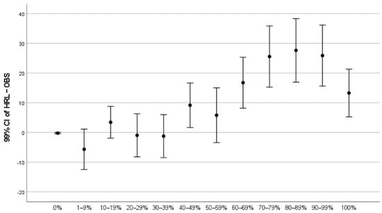
Figure 2.
Mean difference between imperviousness reported by IMD and observed in orthophoto together with the 99% CI of these mean differences.
Figure 2 reveals a small but statistically significant neglect of sealed surfaces in areas where HRL IMD reports no imperviousness. The results show good accuracy for land with imperviousness above 0% and up to 40%. The imperviousness on land where the imperviousness is above 40% is often overestimated in HRL IMD, and the error is increasing as the imperviousness increases. The overestimation is high but stable for land where the imperviousness is in the range 70–99%. The estimate is better again, although still high, for land assessed as 100% impervious by HRL IMD.
4. Discussion
This discussion covers four topics. The first topic is the accuracy assessment of HRL IMD. This is followed by a discussion of the within-pixel sampling approach. The third part of the discussion is concerned with alternatives to the within-pixel sampling approach. The final topic is the applicability of the within-pixel sampling approach to other remote sensing products.
4.1. The Accuracy Assessment of HRL IMD
According to Statistics Norway (https://www.ssb.no/statbank/table/10781/, last accessed on 7 June 2022), the physically sealed areas in Norway in 2018 were 167,818 hectares (54,866 hectare covered with buildings or similar constructions and 112,952 hectares road surface). Our survey estimate is around 10% below the figure provided by Statistics Norway. The figure provided by Statistics Norway and the survey estimate both indicate that the figure given by HRL IMD is too low. The estimate provided by HRL IMD is almost 40% below the figure given by Statistics Norway and 33% below the estimate based on aerial photographs.
The data from Statistics Norway are based on official records and are reliable. The two most important sources are the national building register and the roads register. The building register is a complete inventory of buildings in Norway, including information about the ground area of each building. The register is maintained by municipal authorities. The roads register is maintained by the national roads authority and include information about the length, width, and surface material of all roads except logging roads, but logging roads are not paved. The information from these registers is completed with data from municipal authorities documenting parking lots, sports facilities, and other constructions.
Buildings and paved roads in rural areas were frequently classified as non-impervious (0%). There was no obvious pattern behind the omission of these sealed constructions. Part of a road could be marked as impervious, another part as non-impervious. The buildings on one farm could show up as impervious, while the entire farmstead of the next farm was marked as non-impervious. Neither the width of the roads nor the size or substance covering the roof of buildings could explain this variation.
Impervious surfaces below overhanging trees were occasionally mapped as non-impervious in HRL IMD. Examples are smaller buildings (cabins) inside forests and roads running through densely forested areas. This was also sometimes seen in residential neighborhoods with large gardens, where old trees developed an overhanging canopy partially covering constructions underneath.
The inclusion errors could be grouped into (a) permeable areas wrongly classified as impervious, and (b) situations where the size of the area sealed by constructions was overestimated. The latter situation appeared to be an extrapolation of sealed surfaces due to shadows cast by buildings and roadcuts.
Logged timber is stockpiled next to logging roads, awaiting transport to terminals, sawmills and industrial sites where large amounts of logs are stowed while waiting for further transport or processing. These stacks of lumber are frequently registered as impervious land in HRL IMD.
A similar effect is seen in places producing firewood used for heating houses during the cold season. Many farmers produce large quantities of firewood which is sold to house-owners with no private forest of their own. Production of firewood requires that logs transported from the forest are stockpiled (equivalent to the stacks used in ordinary logging operations, but on a smaller scale). The firewood is stored for drying. The process usually takes a year, and the storage can cover substantial areas which occasionally were mapped as impervious in HRL IMD.
Both natural and artificial gravel surfaces were frequently classified as impervious by HRL IMD. This included areas inside gravel pits and quarries as well as natural gravel, e.g., along riverbeds where gravel and boulders are exposed during the dry part of the summer, and along the edge of reservoirs where bedrock is exposed due to low water level part of the year. Artificial gravel surfaces such as parking spaces, playgrounds and sports fields covered with subbus or pebbles of variable grain size were also occasionally mapped as impervious in HRL IMD.
A particular phenomenon were floating docks found in marinas for yachts and smaller boats. They are hard surfaces and registered as impervious in HRL IMD.
According to the technical documentation of HRL IMD [28] railway tracks associated to other impervious surfaces (i.e., inside built-up areas) are impervious while railway tracks not associated to other impervious surfaces (i.e., outside built-up area) are non-impervious. Railway tracks were often represented as impervious in HRL IMD, irrespective of the surrounding environment. Sleepers do represent a perceptible impervious element along the railway track, and the technical documentation should probably be revised accordingly.
Other permeable features frequently reported as impervious are hydropower dams, road cuts, junkyards, parked cars, and silage balls. Dams and road cuts are examples of exposed rock and gravel erroneously classified as impervious. Junkyards, parked cars, and silage are hard surfaces observed by the satellite imagery but should probably not be counted as impervious areas. Junkyards are found in urban as well as rural areas. It can be abandoned industrial sites or farmyards littered with old cars, containers, and other junk. It is probably impossible to classify these areas correctly using satellite imagery.
Parked cars have the same effect as junk. They are interpreted as impervious surfaces. This is not a problem when the cars are parked on an otherwise sealed surface, but parking lots can also be covered by penetrable materials, e.g., gravel.
The silage produced by farmers when meadows are mowed is packed in large balls and wrapped in plastic. The balls are typically assembled in one part of the field and left there until the fodder is needed. The plastic cover around these balls is impenetrable and stacks of silage balls can be seen as impervious areas in HRL IMD.
A final source of error is the deep and dark shadows between or next to buildings and roadcuts. These are sometimes also interpreted as impervious land and inflates the reported imperviousness degree of built-up land.
These results are largely in agreement with results found in other countries. Two studies of HRL IMD products for Poland found that sealed surfaces were omitted in rural areas while imperviousness was overestimated in built-up areas. The omissions were identified as small buildings, narrow roads, etc., which were treated as natural surfaces. Trodden and ridden areas, on the other hand, could appear as impervious. These studies list industrial areas, dirt-roads or dirt-courtyards and areas covered with bare soil as examples of land wrongly assigned an imperviousness above 0% [31,32].
A similar study of the HRL IMD product for Slovakia describes the overall accuracy as acceptable but found that imperviousness tended to be overestimated in areas where soil sealing was regular and underestimated in areas where soil sealing was sporadic. As a result, the proportion of impervious surfaces could be overestimated in urban areas and underestimated or neglected among rural settlements [33].
The interpretation of errors or mistakes in HRL IMD in the current study is based on observations made during the within-pixel sampling. This is an unsystematic approach with respect to errors but may still provide useful information about the data. Systematic studies of the suspected mistakes can be designed based on these observations.
The two most important findings from the accuracy assessment are the apparently unsystematic omission of sealed land in rural areas and the systematic overestimation of imperviousness degree in the most densely built-up areas. Both observations comply with results from other studies, and both indicate that there are challenges regarding the calibration of the model used in the production of HRL IMD. Dedicated studies are needed to quantify these problems and improve the model.
4.2. The Sampling Methodology
This study employed a two-stage sampling strategy to examine HRL IMD. The first stage was a stratified random sample of pixels. The second stage was a systematic point sample within each of the pixels selected at the first stage. Within-pixel sampling will always require two stages, since pixels must be selected for examination before the within-pixel sample can be established, but a simple random sample will usually be sufficient at the first stage.
The decision to use a stratified approach at the first stage was related to the data distribution. The situation with 99.4% of the pixels having 0% imperviousness required special treatment. This skewed distribution of imperviousness data is not unique for Norway, but has also been reported for other countries, among them Poland [31].
The sample of pixels with 0% imperviousness had to be large enough to detect mistakes inside this group. The sample from the remaining pixels (1–100% imperviousness) had to cover the entire range of values and be large enough to represent variation inside each stratum. Finally, the sampling strategy had to be realistic within the available budget. Stratified sampling met these requirements, but only by using an unbalanced sample.
A stratified sample should preferably be a balanced sample. A balanced sample is a sample where the sample size in each stratum is proportional to the size of the stratum, i.e., ni/n = Ni/N. This was not possible within the constraints of a realistic sample size.
With 99.4% of the pixels in a single stratum, a balanced sample of 2000 pixels implies that 1988 sample points should be drawn from this stratum alone and only twelve sample points from the pixels with imperviousness > 0%. An unbalanced sample was therefore necessary. A balanced sample would have been preferred if the distribution (of imperviousness values) had been more uniform across the entire range from 0% to 100%. Stratified sampling as well as the unbalanced configuration of strata used in this study are choices justified by the properties of the data being examined and should not be interpreted as general recommendations.
Each pixel selected in the first stage was examined using a systematic sample of 100 sample points inside the pixel (Figure 1). The preconditions for this methodology are the availability of high-resolution orthophoto geometrically aligned with the raster and GIS software that allows for efficient and accurate data collection. The approach was efficient and did provide interesting results, but there were also obvious shortcomings and questions that need to be resolved.
The sample size was set to 100 sample points per pixel. The sample size was chosen due to convenience. The 100 sample points allowed the sample points to be placed one meter apart. This appeared to be a dense sample inside a single 10 m pixel. Proportions could also be calculated without effort. Any sample size could have been used, but smaller samples inside each pixel would weaken the statistical support of the analysis.
The number of pixels examined could have been increased by reducing the sample size inside each pixel. The number of pixels could probably have been increased from 2082 to approximately 8000 by cutting the number of sample points inside pixels from 100 down to 25 (points two meters apart). The effect in terms of accuracy has not been examined. This should be performed to provide better advice about the optimum balance between sample sizes in the first and the second sampling stage.
A systematic random sample was used for sampling inside each pixel. A systematic sample is known to provide more accurate estimates than a simple random sample of the same size when spatial autocorrelation is present in the material [30]. Spatial autocorrelation with respect to imperviousness implies that the sealed area tends to be clustered in certain parts of the pixel rather than distributed randomly over the surface of the pixel. The assumption is justified because soil sealing is caused by constructions.
There is, however, no exact method to calculate the statistical accuracy of a systematic sample. The accuracy must be determined by estimation [34]. A conservative estimate of the uncertainty in a systematic sample can be found by treating the sample as a simple random sample, but the result is that the improved accuracy achieved by the systematic approach goes unnoticed. Trials with forestry data has shown that a systematic sample can reduce uncertainty with as much as 30% when autocorrelation is present [35]. This improvement should be documented. Several estimation methods have been published [36,37] and could be applied to within-pixel sampling. A common requirement is, however, that the (relative) location of each sample point in the systematic sample must be recorded.
The systematic sample within pixels could have been replaced by a simple random sample. The disadvantage, apart from the assumed lower precision, is that a simple random sample may be more difficult to observe when the sample size is large. This assumption has not been tested, but it seems more challenging to work with a completely random distribution of points than counting along a regular lattice with the same number of points.
Finally, by experience, even the resolution of high quality orthophoto is insufficient to allow exact interpretation of impervious vs. permeable parts of the pixel surface. The pixel shown in Figure 1 contains a road, a roadside ditch, and part of an agricultural field. The edge between the solid and the permeable surface is somewhere along the white line painted beside the road, but it is not possible to tell exactly where the edge is. Consequently, the accuracy of the data obtained by sampling within pixels also depend on the quality of the orthophoto and the experience of the analyst [38].
Within-pixel sampling was found to be suitable for accuracy assessment of HRL IMD, but more work is clearly needed to improve the methodology. Geometrical inconsistencies between the raster and the aerial imagery used as ground truth will make the results uncertain or even meaningless, as will interpretation errors with respect to ground truth. The sampling accuracy at stage two was disregarded in this study and replaced by a conservative interpretation of the sampling error at stage one. Better tools are needed to handle the systematic sample and estimate the sampling accuracy inside each pixel.
4.3. Alternative Approaches
A complete inventory of each control pixel is an alternative to the within-pixel sampling approach. Such an inventory could be carried out as a ground survey, but the cost would be excessive. Digitizing from orthophoto or by photogrammetric construction using stereo photography are manageable, but still expensive alternatives. A complete inventory will eliminate the sampling error generated by the second stage of the survey.
Another alternative is a simplified accuracy assessment using a classified version of the dataset. This approach has been used in several unpublished, national verification reports commissioned by EEA. HRL IMD is reclassified into three classes (“0%”, “1–29%” and “30–100%”). A stratified sample of control pixels is selected, and a qualitative assessment (based on available imagery) is used to assign the pixels to one of the three simplified classes. The approach allows for calculation of omission and commission errors between the three classes using standard methodology [39,40].
None of these alternatives will remove the observation error and inaccuracies stemming from geometrical misalignment between the data sources, but both alternatives eliminate the sampling error of the within-pixel sampling approach. The complete inventory is probably expensive, even with on-screen digitizing, while the assessment of a simplified version of the product results in drastic reduction in the information obtained from the accuracy assessment.
4.4. Applicability to Other Remote Sensing Products
The within-pixel sampling strategy used in the present study is suitable for assessment of a remote sensing product that represents a binomial proportion. Examples are imperviousness and canopy coverage. Within-pixel sampling may be less suitable for other remote sensing products.
Binary remote sensing products show the presence or absence of a particular feature. An example is the Copernicus high-resolution layer grassland [41] showing the presence or absence of grassland. A binary remote sensing product is essentially a simplified version of a binomial proportion. Sampling within pixels is suitable for assessment of these products provided that the decision rules used in the classification of the pixel are clearly expressed. Examples of decision rules can be that the feature must be present in the pixel, cover a defined proportion of the pixel surface, or dominate the pixel. Correct classification can then be assessed by within-pixel sampling.
Within-pixel sampling is less suitable for assessment of categorical remote sensing products (e.g., land cover maps and crop type maps) unless the classes are scale-independent, pure land cover classes and the decision rules used to classify pixels are known (e.g., crop type determined by the dominant crop type in the pixel). Scale-dependent classifications and classifications involving elements of land use will be difficult to assess by within-pixel sampling.
Within-pixel sampling can, on the other hand, be used for descriptive analysis aiming to improve the explanation of the classes used in a categorical remote sensing product. Descriptive analysis does not assess accuracy but describes the content of classes in terms of more detailed data. An example is the analysis of the content of the European CORINE Land Cover Map by populating the classes with data from more detailed map sources [42]. Within-pixel sampling of pure land cover elements can be used for this purpose.
5. Conclusions
One objective of the current study was to examine the content and accuracy of the high-resolution layer imperviousness density (HRL IMD) product for 2018. Norway was used as the study area. There was a noteworthy neglection of buildings and roads in rural areas. The effect of these omissions was to some extent reduced by overestimation of the imperviousness density in built-up areas. Overall, the amount of sealed surface estimated from HRL IMD was 33% below the amount estimated using high-resolution orthophoto and 40% below the official figure on sealed surface published by Statistics Norway.
The results indicate that the statistics provided by HRL IMD is biased because the omissions of sealed surfaces in rural areas were larger (in absolute terms) than the inclusion errors in built-up areas. It is reasonable to expect that the ratio between built-up and natural land, along with the zoning structure has an impact on the bias and that the errors may be more balanced in regions with more built-up land. Still, bias is present and further work is needed to improve the model used in the production of HRL IMD, aiming to reduce or even eliminate the bias.
The Copernicus land monitoring services (CLMS), including HRL IMD, are standardized products covering all of Europe, but the quality and accuracy are likely to vary across the continent. The products can still be valuable for comparative studies. Time series can provide useful information on changes, provided that the errors are randomly distributed [43]. Authors have also found the products useful for comparing locations, as in the comparative study of suburban patterns in the Barcelona and Milan [44] and as a tool to decompose less detailed data sets, such as CORINE Land Cover [45,46].
The findings from the current study can be used to improve the interpretation and understanding of the product. The user should be aware that bias is present in the material and understand how the errors are distributed between land systems when the results are interpreted. Accuracy assessment and verification studies from various subregions of Europe are therefore needed to establish product credibility when HRL IMD and other CLMS data are incorporated into decision systems, especially at local administrative levels [47]. Interpretative studies of the data provided by the Copernicus land monitoring services should therefore be an integral part of the program.
The within-pixel sampling strategy used in the study was found suitable for assessment of imperviousness. It is probably also appropriate for assessment of other binomial proportions. The study did, however, reveal challenges that require further methodological studies and development. This was linked to the use of systematic random sampling within pixels.
A systematic sample inside each pixel is easy to work with and is known to produce more accurate estimates than a simple random sample when spatial autocorrelation is present. The improvement in accuracy does, however, go unnoticed unless the status and location of each sample point inside the pixel is recorded and an appropriate method is applied to estimate the accuracy. These methods exist but functional tools must be developed. Further research is also needed to help determine the optimal sample sizes at the different stages of a survey.
Funding
The research leading to these results received funding from the Norway Grants 2014–2021 via the Polish National Center for Research and Development [grant no: NOR/POLNOR/InCoNaDa/0050/2019-00] and was partly carried out by the joint Polish-Norwegian project Integration of Copernicus and National Data (InCoNaDa).
Data Availability Statement
HRL IMD can be downloaded from https://land.copernicus.eu and the reference data can be inspected at https://kilden.nibio.no. The sample can be obtained from the author.
Conflicts of Interest
The author declares no conflict of interest. The funders had no role in the design of the study; in the collection, analyses, or interpretation of data; in the writing of the manuscript, or in the decision to publish the results.
References
- Meyer, W.B.; Turner, B.L. Human population growth and global land-use/cover change. Annu. Rev. Ecol. Syst. 1992, 23, 39–61. [Google Scholar] [CrossRef]
- Jennings, D.B.; Taylor Jarnagin, S. Changes in anthropogenic impervious surfaces, precipitation and daily streamflow discharge: A historical perspective in a mid-Atlantic subwatershed. Landsc. Ecol. 2002, 17, 471–489. [Google Scholar] [CrossRef]
- Burghardt, W. Soil sealing and soil properties related to sealing. Geol. Soc. Lond. Spec. Publ. 2006, 266, 117–124. [Google Scholar] [CrossRef]
- Arnold, C.L., Jr.; Gibbons, C.J. Impervious surface coverage: The emergence of a key environmental indicator. J. Am. Plan. Assoc. 1996, 62, 243–258. [Google Scholar] [CrossRef]
- Shuster, W.D.; Bonta, J.; Thurston, H.; Warnemuende, E.; Smith, D.R. Impacts of impervious surface on watershed hydrology: A review. Urban Water J. 2005, 2, 263–275. [Google Scholar] [CrossRef]
- Jacobson, C.R. Identification and quantification of the hydrological impacts of imperviousness in urban catchments: A review. J. Environ. Manag. 2011, 92, 1438–1448. [Google Scholar] [CrossRef] [PubMed]
- Tobias, S.; Conen, F.; Duss, A.; Wenzel, L.M.; Buser, C.; Alewell, C. Soil sealing and unsealing: State of the art and examples. Land Degrad. Dev. 2018, 29, 2015–2024. [Google Scholar] [CrossRef]
- Li, J.; Pei, Y.; Zhao, S.; Xiao, R.; Sang, X.; Zhang, C. A review of remote sensing for environmental monitoring in China. Remote Sens. 2020, 12, 1130. [Google Scholar] [CrossRef]
- Slonecker, E.T.; Jennings, D.B.; Garofalo, D. Remote sensing of impervious surfaces: A review. Remote Sens. Rev. 2001, 20, 227–255. [Google Scholar] [CrossRef]
- Yang, L.; Huang, C.; Homer, C.; Wylie, B.; Coan, M. An approach for mapping large-area impervious surfaces: Synergistic use of Landsat 7 ETM+ and high spatial resolution imagery. Can. J. Remote Sens. 2002, 29, 230–240. [Google Scholar] [CrossRef]
- Homer, C.; Huang, C.; Yang, L.; Wylie, B.; Coan, M. Development of a 2001 national land-cover database for the United States. Photogramm. Eng. Remote Sens. 2004, 70, 829–840. [Google Scholar] [CrossRef]
- Raymaekers, D.; Bauwens, I.; Van Orshoven, J.; Gulinck, H.; Engel, B.; Dosselaere, N. Spectral unmixing of low resolution images for monitoring soil sealing. In Urban 2005, Proceedings of the 3rd International Symposium Remote Sensing and Data Fusion Over Urban Areas, Tempe, AZ, USA, 14–16 March 2005; ISPRS: Hannover, Germany, 14–16 March 2005. [Google Scholar]
- Kampouraki, M.; Wood, G.A.; Brewer, T.R. The application of remote sensing to identify and measure sealed areas in urban environments. In Bridging Remote Sensing and GIS, Proceedings of the 1st International Conference on Object-Based Image Analysis, Salzburg, Austria, 4–6 June 2006; ISPRS: Hannover, Germany, 2006. [Google Scholar]
- Kampouraki, M.; Wood, G.A.; Brewer, T.R. The suitability of object-based image segmentation to replace manual aerial photo interpretation for mapping impermeable land cover. In Challenges for Earth Observation: Scientific, Technical and Commercial, 426–430, Proceedings of the Remote Sensing and Photogrammetry Society Annual Conference, Newcastle Upon Tyne, UK, 11–14 September 2007; Heipke, C., Ed.; Remote Sensing and Photogrammetry Society (RSPSoc): Nottingham, Germany, 2007. [Google Scholar]
- Weng, Q. Remote sensing of impervious surfaces in the urban areas: Requirements, methods, and trends. Remote Sens. Environ. 2012, 117, 34–49. [Google Scholar] [CrossRef]
- Salvati, L. The spatial pattern of soil sealing along the urban-rural gradient in a Mediterranean region. J. Environ. Plan. Manag. 2014, 57, 848–861. [Google Scholar] [CrossRef]
- Kuc, G.; Chormański, J. Sentinel-2 imagery for mapping and monitoring imperviousness in urban areas. The International Archives of Photogrammetry. Remote Sens. Spat. Inf. Sci. 2019, 42, 43–47. [Google Scholar] [CrossRef]
- Shrestha, B.; Ahmad, S.; Stephen, H. Fusion of Sentinel-1 and Sentinel-2 data in mapping the impervious surfaces at city scale. Environ. Monit. Assess. 2021, 193, 556. [Google Scholar] [CrossRef]
- Peroni, F.; Pappalardo, S.E.; Facchinelli, F.; Crescini, E.; Munafò, M.; Hodgson, M.E.; De Marchi, M. How to map soil sealing, land take and impervious surfaces? A systematic review. Environ. Res. Lett. 2022, 17, 053005. [Google Scholar] [CrossRef]
- Moglen, G.E.; Kim, S. Limiting imperviousness: Are threshold-based policies a good idea? J. Am. Plan. Assoc. 2007, 73, 161–171. [Google Scholar] [CrossRef]
- Parent, J.R.; Lei, Q. Estimating percent impervious cover from Landsat-based land cover with a simple and transferable regression model. Int. J. Remote Sens. 2018, 39, 3839–3851. [Google Scholar] [CrossRef]
- Lefebvre, A.; Sannier, C.; Corpetti, T. Monitoring urban areas with Sentinel-2A data: Application to the update of the Copernicus high resolution layer imperviousness degree. Remote Sens. 2016, 8, 606. [Google Scholar] [CrossRef]
- European Environment Agency. The European Environment—State and Outlook 2020. Knowledge for Transition to a Sustainable Europe; Publications office of the European Union: Luxembourg, 2019.
- Vysna, V.; Maes, J.; Petersen, J.E.; La Notte, A.; Vallecillo, S.; Aizpurua, N.; Ivits, E.; Teller, A. Accounting for ecosystems and their services in the European Union (INCA). Final Report from Phase II of the INCA Project Aiming to Develop a Pilot for an Integrated System of Ecosystem Accounts for the EU; Statistical Report; Publications office of the European Union: Luxembourg, 2021.
- Congedo, L.; Sallustio, L.; Munafò, M.; Ottaviano, M.; Tonti, D.; Marchetti, M. Copernicus high-resolution layers for land cover classification in Italy. J. Maps 2016, 12, 1195–1205. [Google Scholar] [CrossRef]
- Smith, G. GMES Initial Operations/Copernicus Land Monitoring Services—Validation of Products. HRL Imperviousness Degree 2015 Validation Report. GIO HRL IMD Validation Report SC03, Issue D1.3. 2019. Available online: https://land.copernicus.eu/user-corner/technical-library/hrl-imperviousness-2015-validation-report (accessed on 7 June 2022).
- Wickham, J.D.; Stehman, S.V.; Gass, L.; Dewitz, J.; Fry, J.A.; Wade, T.G. Accuracy assessment of NLCD 2006 land cover and impervious surface. Remote Sens. Environ. 2013, 130, 294–304. [Google Scholar] [CrossRef]
- Steidl, M.; Schleicher, C.; Sannier, C. Copernicus Land Monitoring Service—High Resolution Layer Imperviousness: Product Specifications Document; European Environment Agency: Copenhagen, Denmark, 2018.
- Lohr, S.L. Sampling: Design and Analysis, 2nd ed.; CRC Press: Boka Raton, FL, USA, 2019. [Google Scholar]
- Cochran, W.G. Sampling Techniques, 3rd ed.; John Wiley & Sons: New York, NY, USA, 1977. [Google Scholar]
- Krówczyńska, M.; Soszyńska, A.; Pabjanek, P.; Wilk, E.; Hurbanek, P.; Rosina, K. Accuracy of the soil sealing enhancement product for Poland. Quaest. Geogr. 2016, 35, 89–95. [Google Scholar] [CrossRef][Green Version]
- Pabjanek, P.; Krówczyńsk, M.; Wilk, E.; Miecznikowski1, M. An accuracy assessment of European Soil Sealing Dataset (SSL2009): Stara Miłosna area, Poland—A case study. Misc. Geogr. Reg. Stud. Dev. 2016, 20, 59–63. [Google Scholar] [CrossRef][Green Version]
- Hurbanek, P.; Atkinson, P.M.; Pazur, R.; Rosina, K.; Chockalingam, J. Accuracy of built-up area mapping in Europe at varying scales and thresholds. In Proceedings of the Accuracy 2010, Ninth International Symposium on Spatial Accuracy Assessment in Natural Resources and Environmental Sciences, Leicester, England, 20–23 July 2010; University of Leicester: Leicester, UK, 2010; Volume 385388. [Google Scholar]
- Strand, G.H. A study of variance estimation methods for systematic spatial sampling. Spat. Stat. 2017, 21, 226–240. [Google Scholar] [CrossRef]
- Magnussen, S.; Nord-Larsen, T. Design-consistent model-based variances with systematic sampling: A case study with the Danish national Forest inventory. Commun. Stat. Simul. Comput. 2021, 50, 38–48. [Google Scholar] [CrossRef]
- Aune-Lundberg, L.; Strand, G.H. Comparison of variance estimation methods for use with two-dimensional systematic sampling of land use/land cover data. Environ. Model. Softw. 2014, 61, 87–97. [Google Scholar] [CrossRef]
- Brus, D.J.; Saby, N.P. Approximating the variance of estimated means for systematic random sampling, illustrated with data of the French Soil Monitoring Network. Geoderma 2016, 279, 77–86. [Google Scholar] [CrossRef]
- Strand, G.H.; Dramstad, W.; Engan, G. The effect of field experience on the accuracy of identifying land cover types in aerial photographs. Int. J. Appl. Earth Obs. Geoinf. 2002, 4, 137–146. [Google Scholar] [CrossRef]
- Aronoff, S. The map accuracy report: A user’s view. Photogramm. Eng. Remote Sens. 1982, 48, 1309–1312. [Google Scholar]
- Congalton, R.G. A review of assessing the accuracy of classifications of remotely sensed data. Remote Sens. Environ. 1991, 37, 35–46. [Google Scholar] [CrossRef]
- Available online: https://land.copernicus.eu/pan-european/high-resolution-layers/grassland (accessed on 7 June 2022).
- Aune-Lundberg, L.; Strand, G.H. The content and accuracy of the CORINE Land Cover dataset for Norway. Int. J. Appl. Earth Obs. Geoinf. 2021, 96, 102266. [Google Scholar] [CrossRef]
- Drašković, B.J. Urban expansion of the largest cities in Bosnia and Herzegovina over the period 2000–2018. Geogr. Pannonica 2021, 25. [Google Scholar] [CrossRef]
- Pagliarin, S. Supra-local spatial planning practices and suburban patterns in the Barcelona and Milan urban regions. Land Use Policy 2022, 112, 105816. [Google Scholar] [CrossRef]
- Cole, B.; Smith, G.; Balzter, H. Acceleration and fragmentation of CORINE land cover changes in the United Kingdom from 2006–2012 detected by Copernicus IMAGE2012 satellite data. Int. J. Appl. Earth Obs. Geoinf. 2018, 73, 107–122. [Google Scholar] [CrossRef]
- Rosina, K.; e Silva, F.B.; Vizcaino, P.; Herrera, M.M.; Freire, S.; Schiavina, M. Increasing the detail of European land use/cover data by combining heterogeneous data sets. Int. J. Digit. Earth 2020, 13. [Google Scholar] [CrossRef]
- Manakos, I.; Tomaszewska, M.; Gkinis, I.; Brovkina, O.; Filchev, L.; Genc, L.; Gitas, I.Z.; Halabuk, A.; Inalpulat, M.; Irimescu, A.; et al. Comparison of global and continental land cover products for selected study areas in South Central and Eastern European region. Remote Sens. 2018, 10, 1967. [Google Scholar] [CrossRef]


Publisher’s Note: MDPI stays neutral with regard to jurisdictional claims in published maps and institutional affiliations. |
© 2022 by the author. Licensee MDPI, Basel, Switzerland. This article is an open access article distributed under the terms and conditions of the Creative Commons Attribution (CC BY) license (https://creativecommons.org/licenses/by/4.0/).