
An Improved Vicarious Calibration Method Based on Multi-Grayscale Targets

 ,
,
Abstract
:
1. Introduction
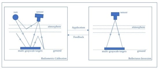
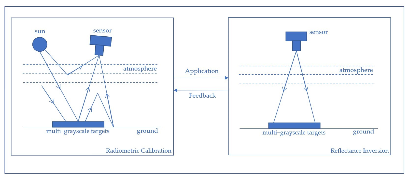
2. Radiometric Calibration-Reflectance Inversion Iterative Model
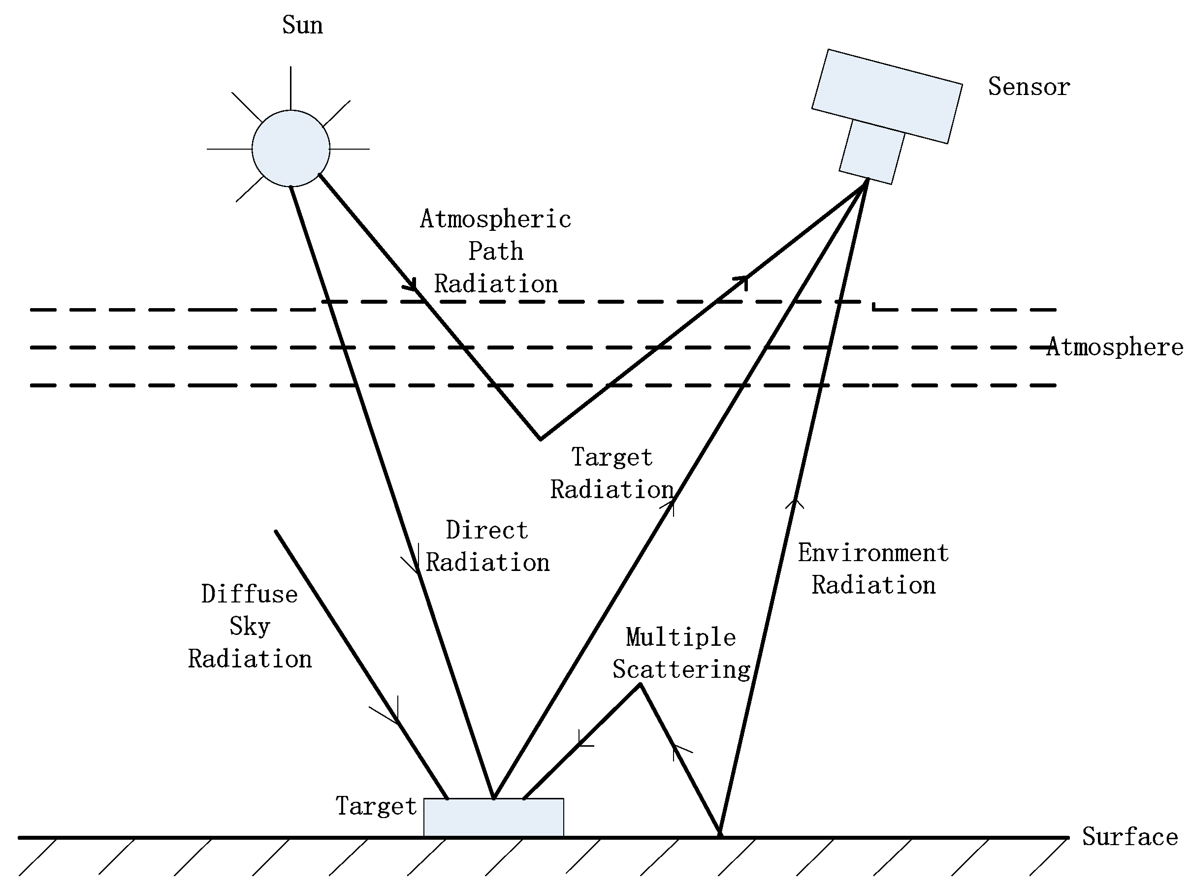
2.1. Radiometric Calibration Model
2.2. Reflectance Inversion Model
- (1)
- In regard to atmospheric absorption and atmospheric path radiation correction of the apparent reflectance image, Equation (2) can be rewritten as:
- (2)
- Choosing any pixel as the target, the reflectance of each pixel can be calculated as follows:
- (3)
- Calculation of the equivalent environmental reflectance
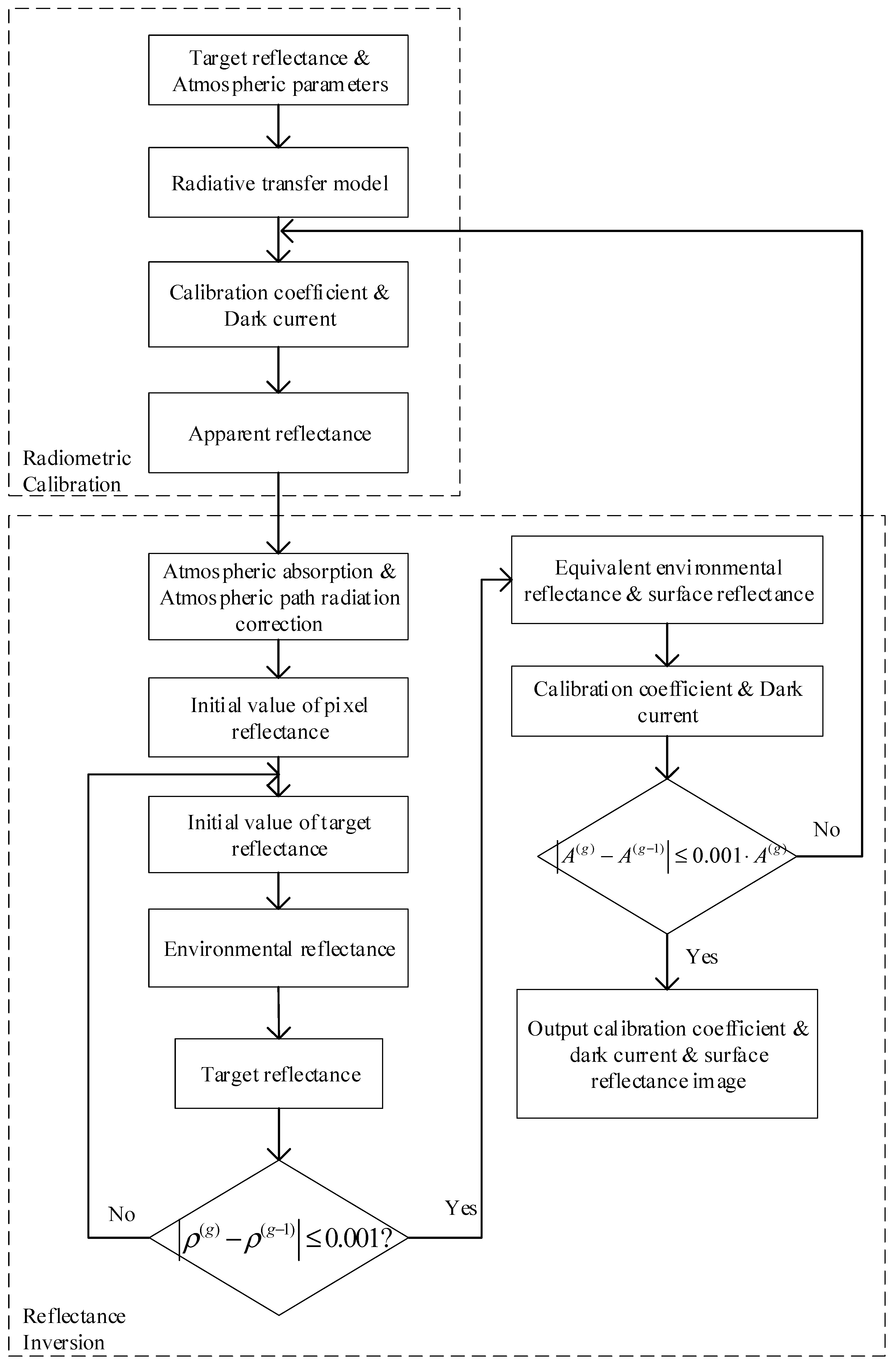
2.3. Radiometric Calibration-Reflectance Inversion Iterative Model
- (1)
- Radiometric calibration is conducted for the grayscale target area, and initial values of the calibration coefficient and dark current are calculated.
- (2)
- The reflectance inversion model described in the above section is applied to the same image to obtain the surface reflectance.
- (3)
- The equivalent environmental reflectance of the target area is determined with the retrieved surface reflectance and substituted into the calibration equation. The calibration coefficient and dark current are again calculated, and reflectance inversion is again performed. The iteration process is repeated a certain number of times until the relative difference between the calibration coefficient and previous iteration result is less than 1‰. Notably, for , the iteration process is terminated. A model flow chart is shown in Figure 2.
3. Experiment and Data Analysis
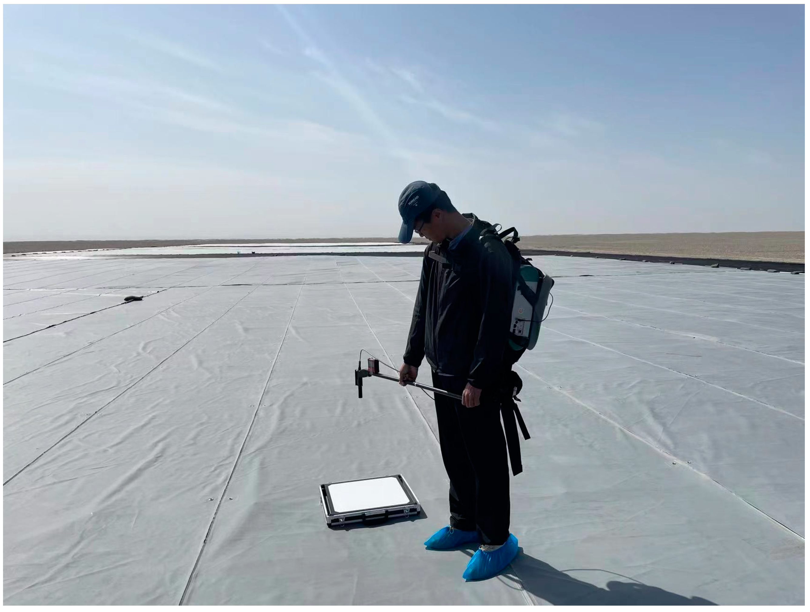
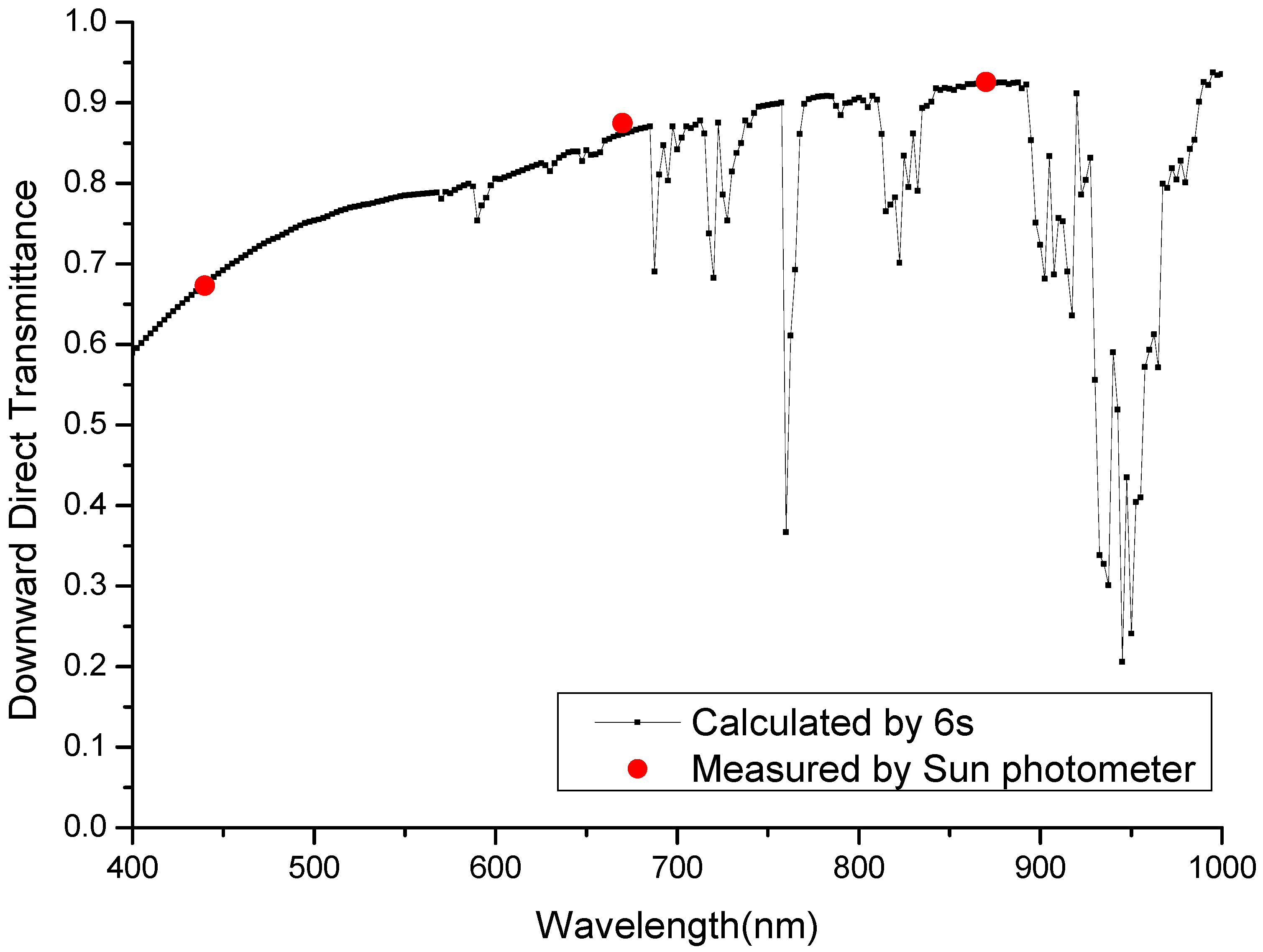
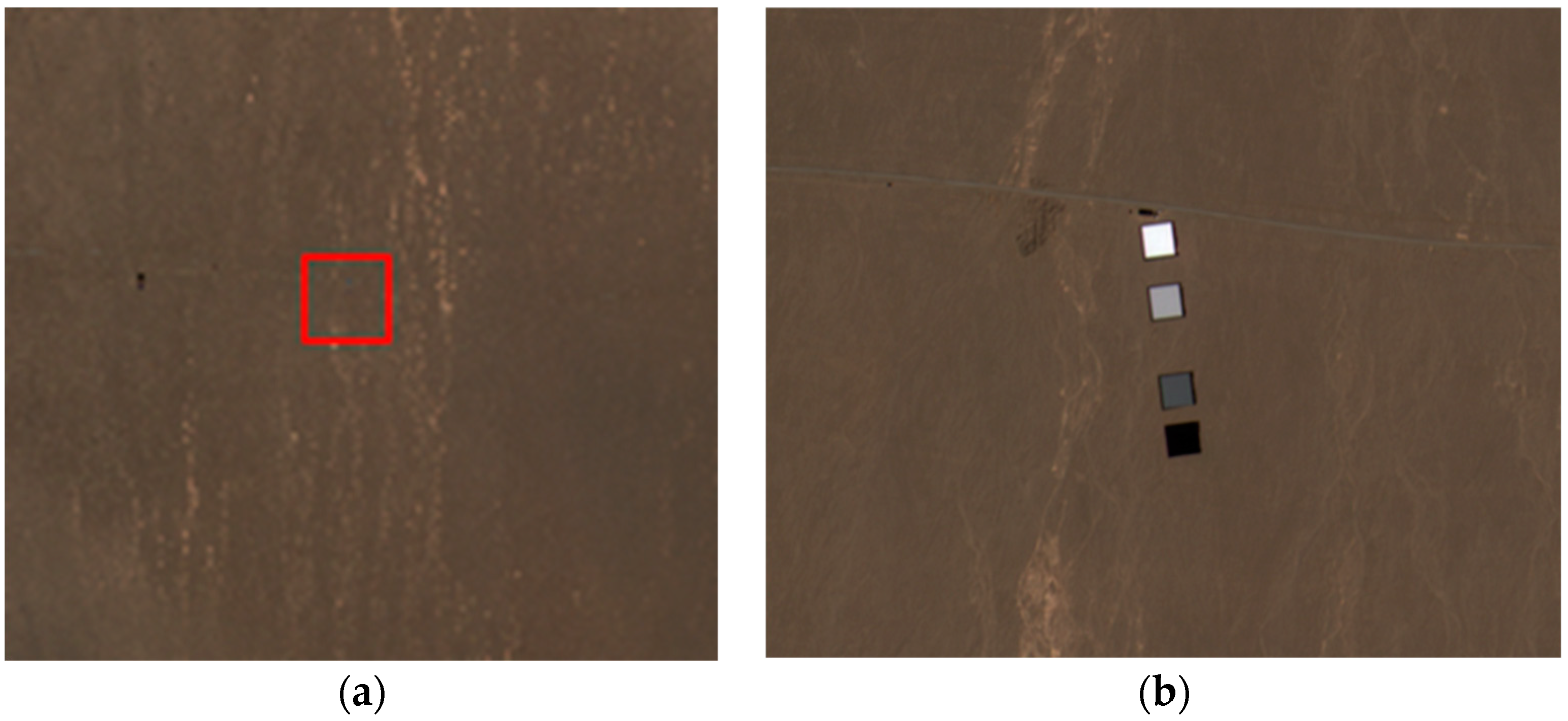
3.1. Experimental Data Measurement
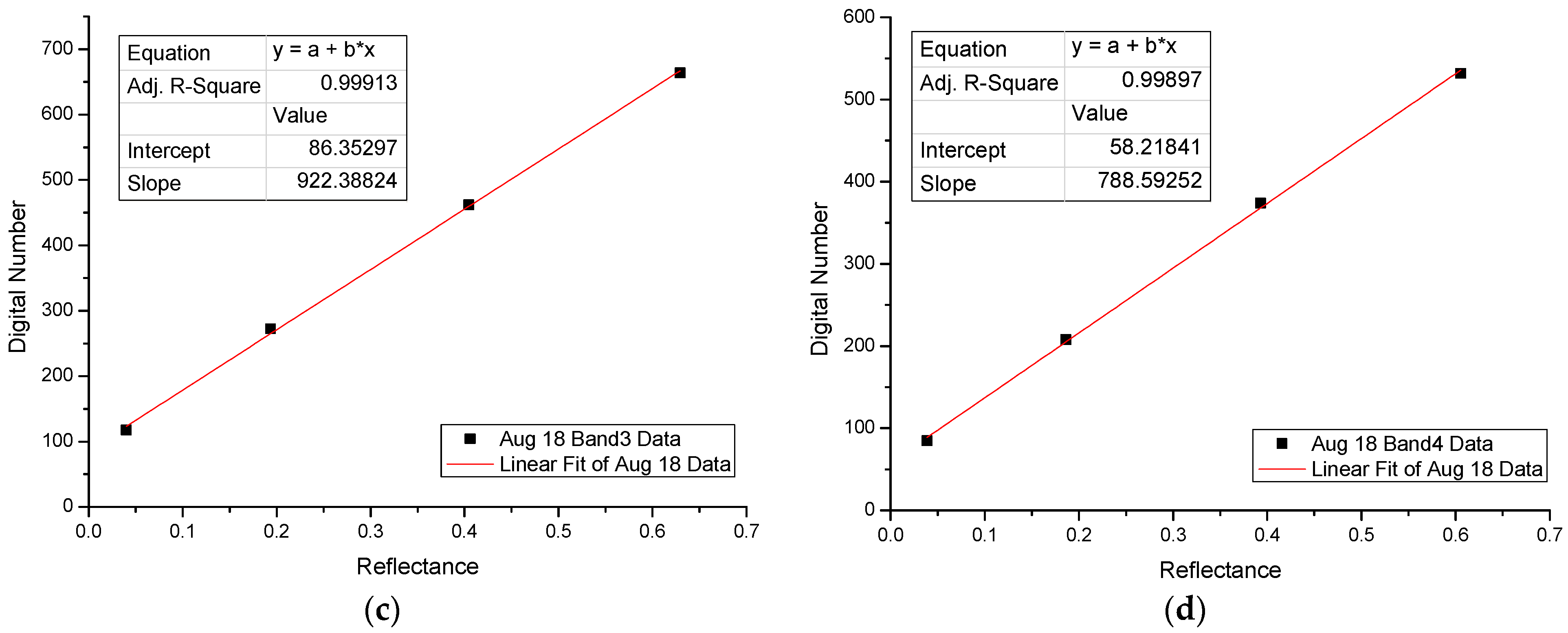
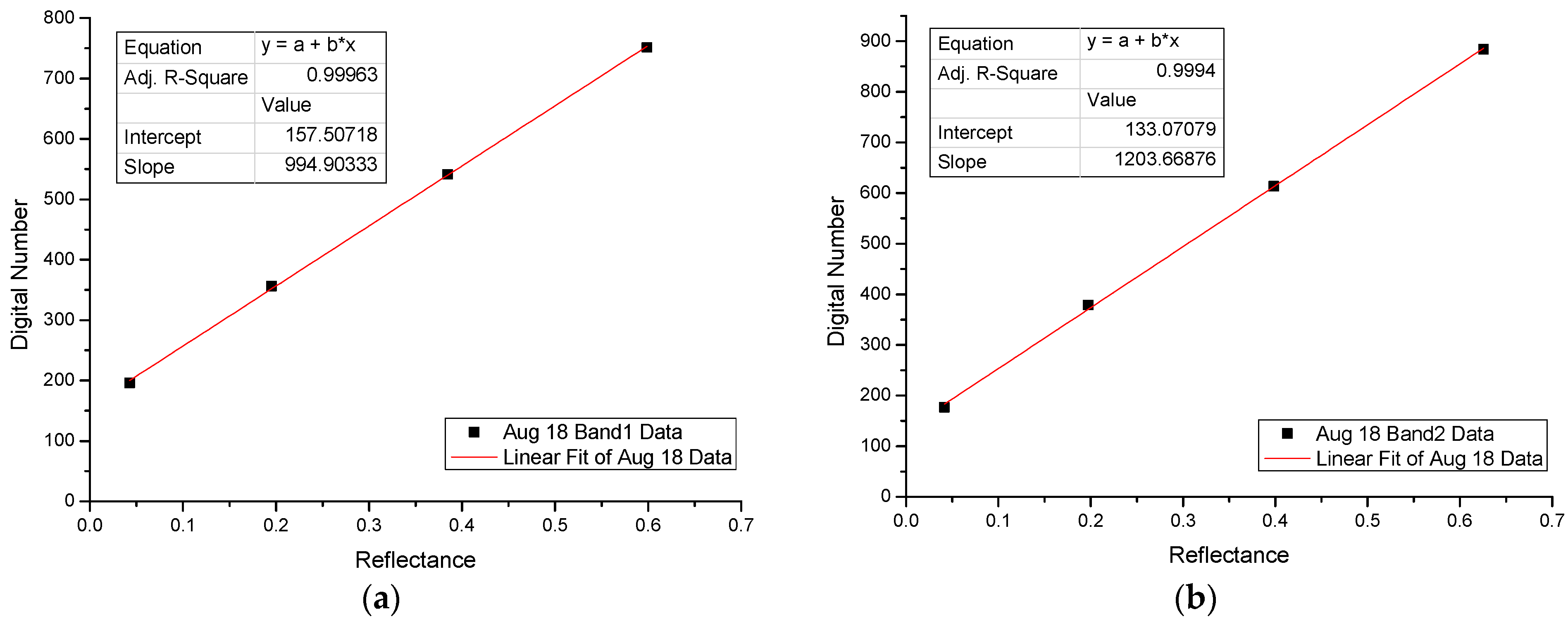
3.2. Calibration Calculation and Reflectance Inversion
4. Method Application
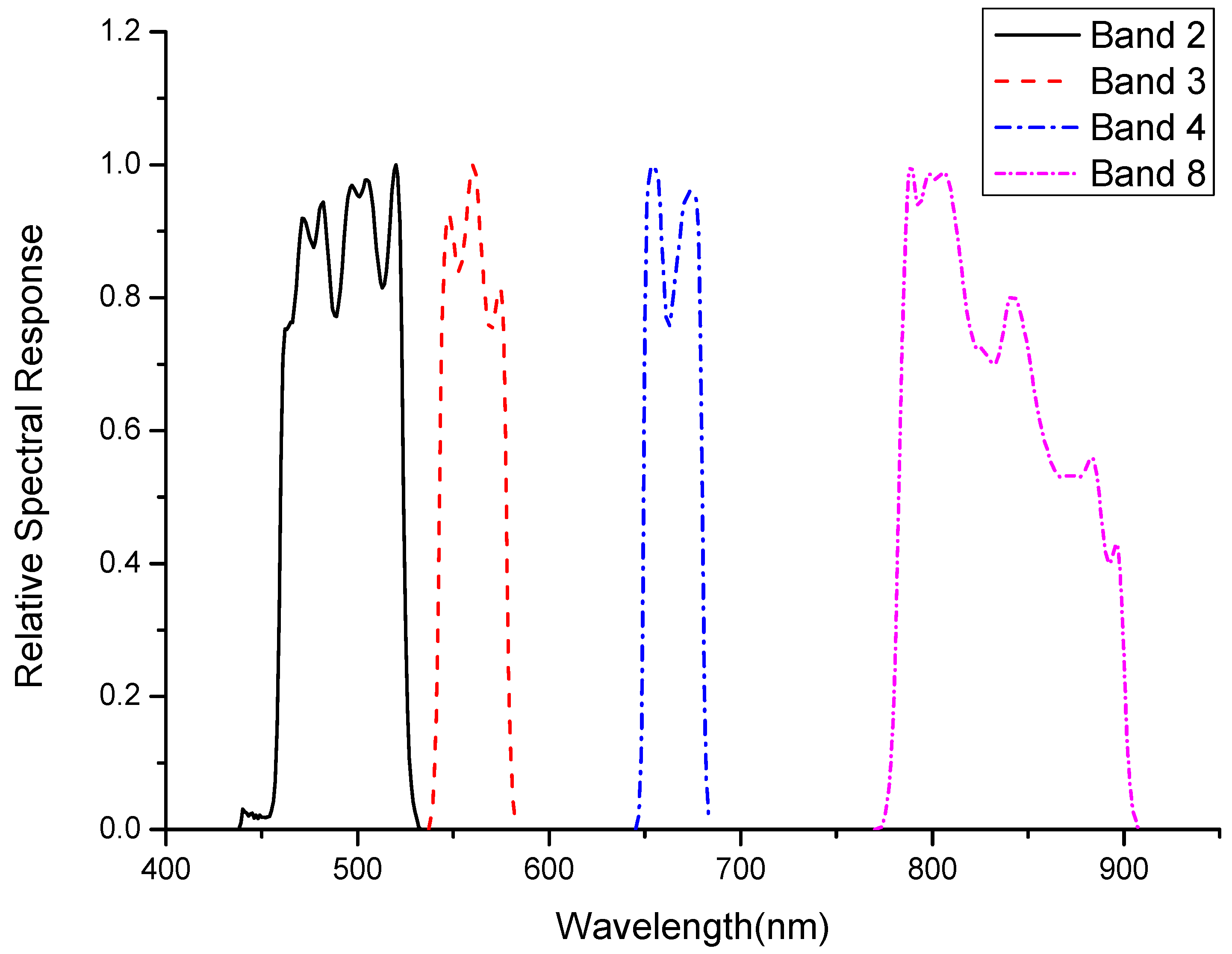
4.1. Top-of-Atmosphere Radiance Cross-Validation
- (1)
- Using 6S radiative transfer model and field measurement parameters, the at-sensor radiance of the two satellites is calculated, respectively; then, the spectral matching factor can be obtained as the ratio of the two.
- (2)
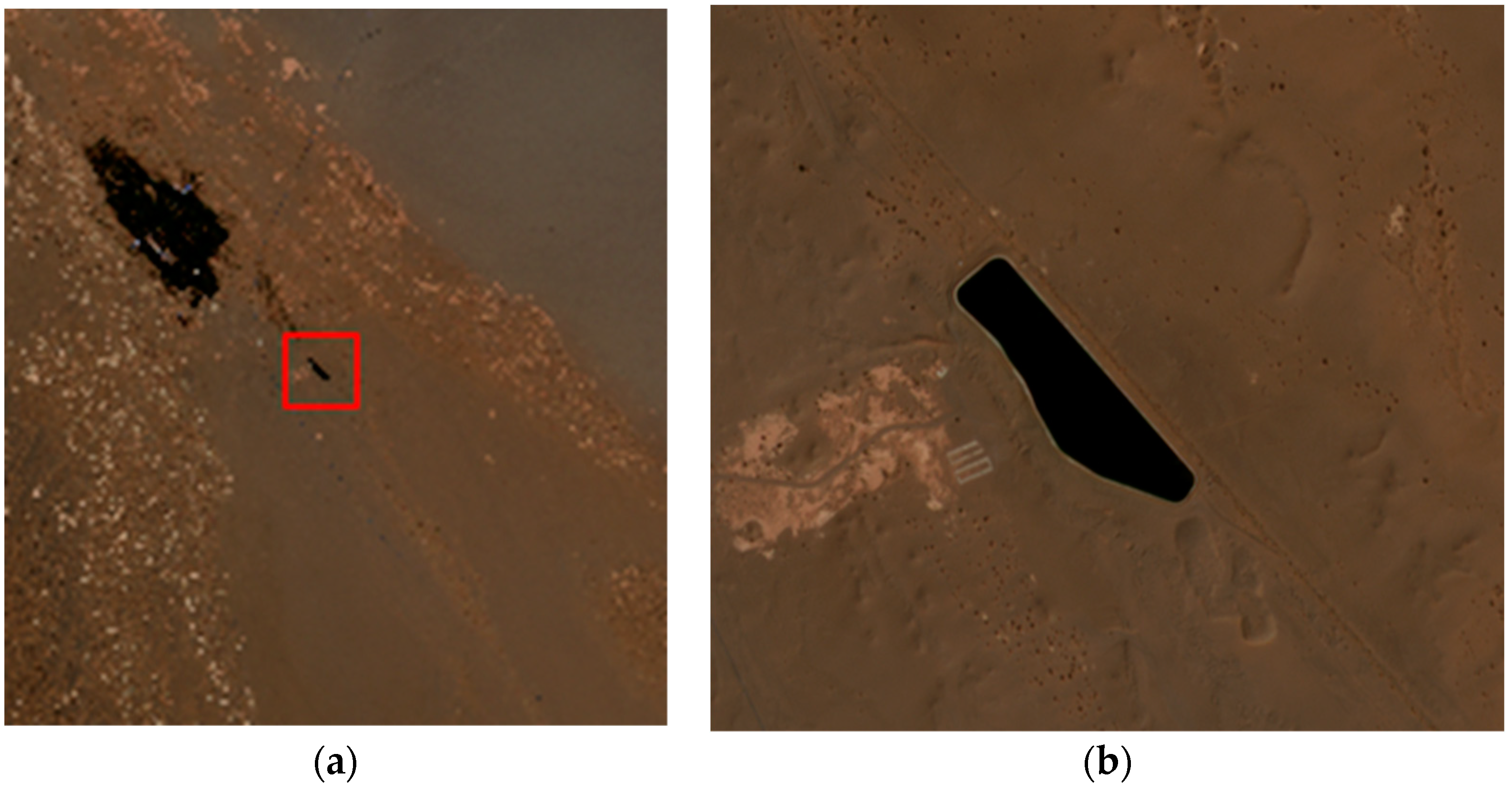
- Take the Gobi on the east side of the target as the crossing object; the PRSS-1 calibration coefficient and offset obtained in the above section is used to calculate the at-sensor radiance by . The at-sensor radiance of Sentinel-2A is directly obtained from the L1C level image.
- (3)
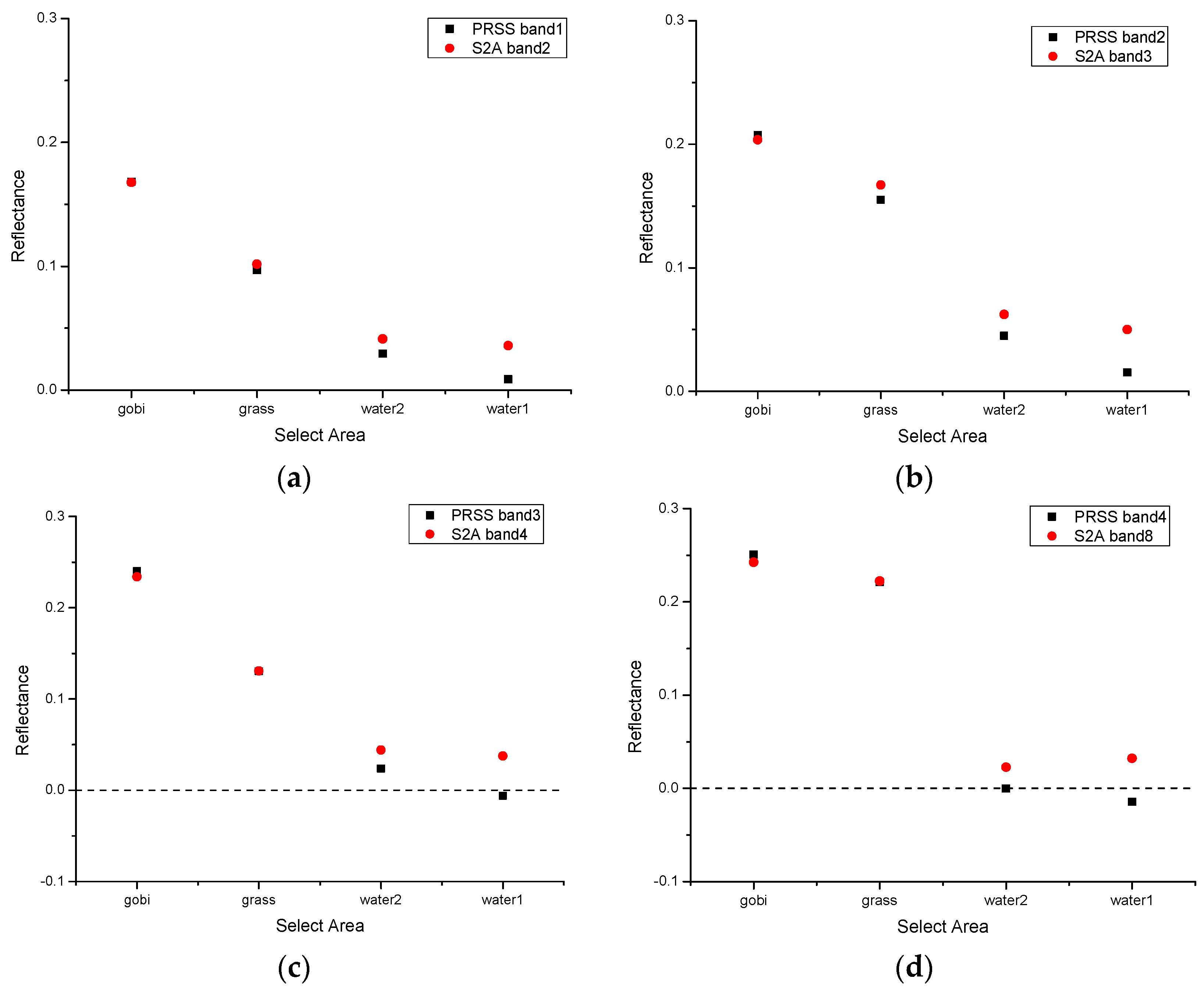
- The at-sensor radiance of PRSS-1 is converted by spectral matching factor and compared with Sentinel-2A.
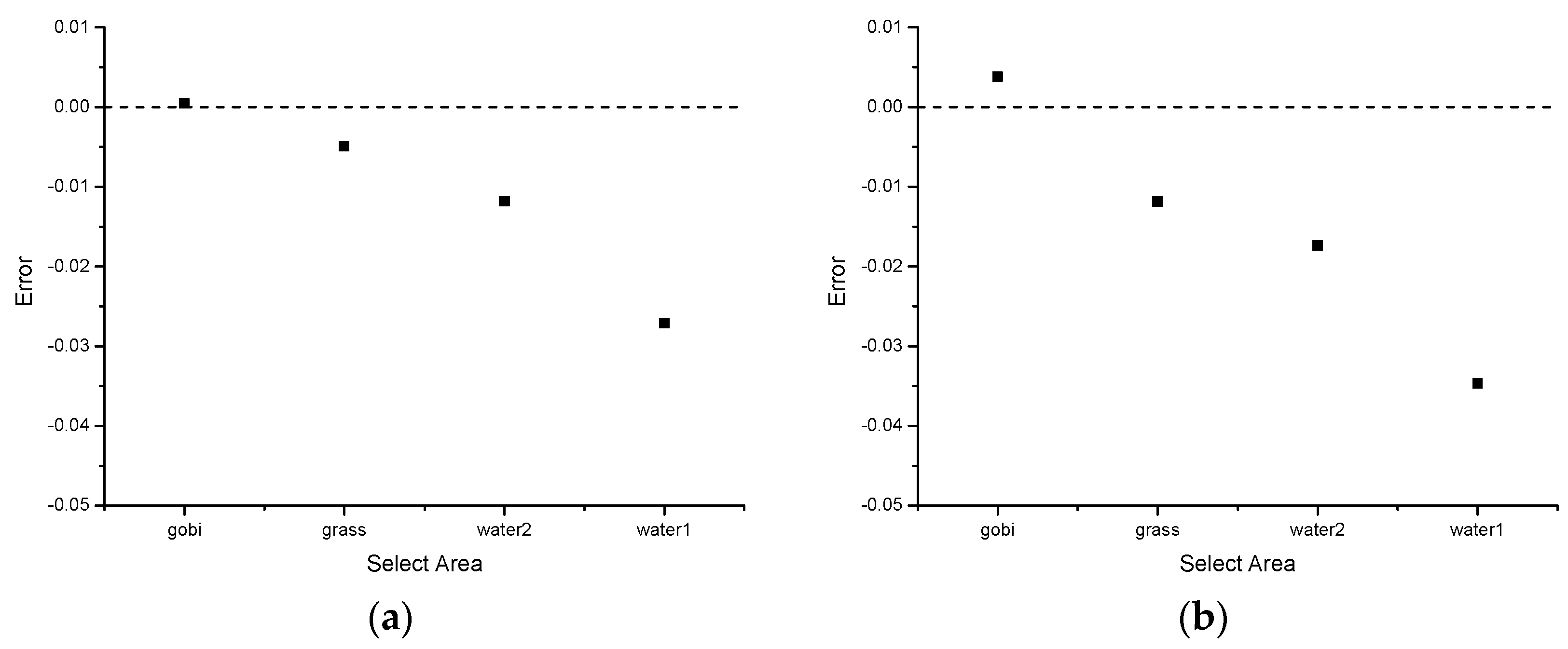
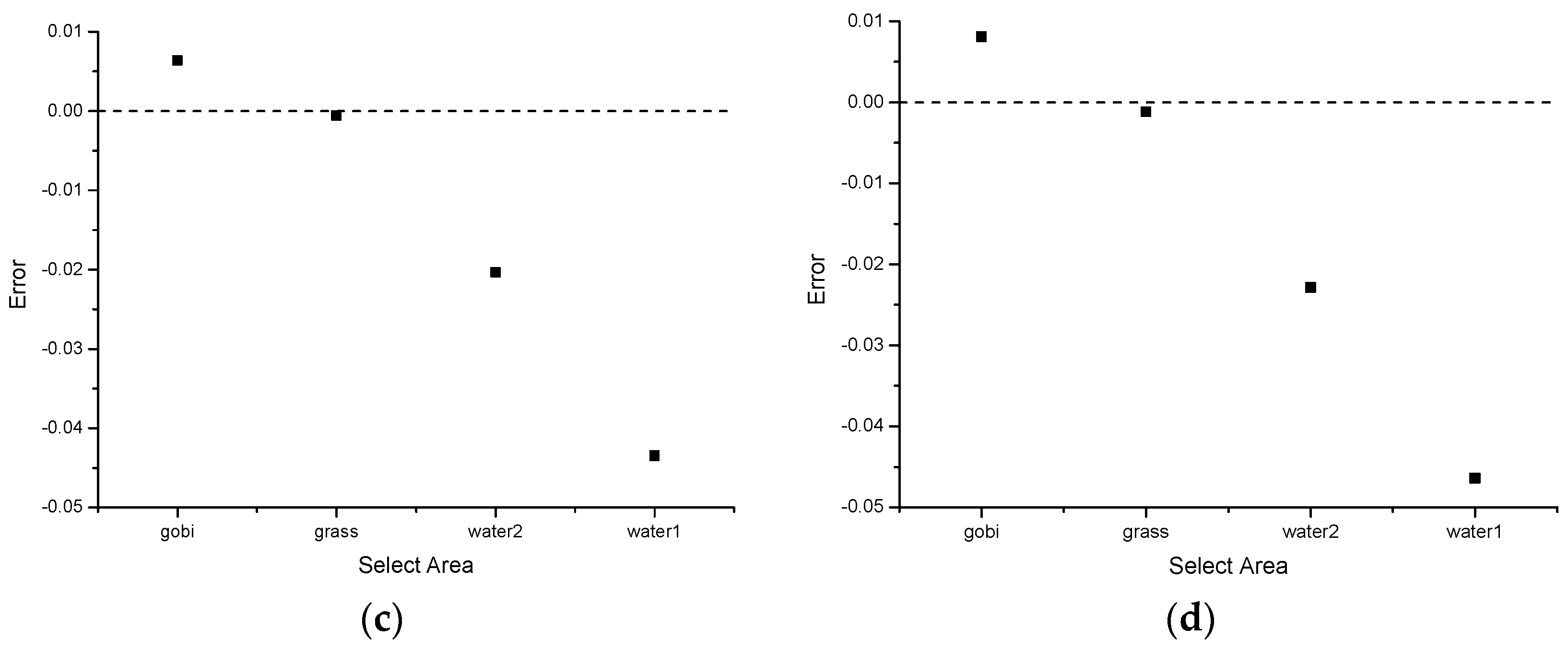
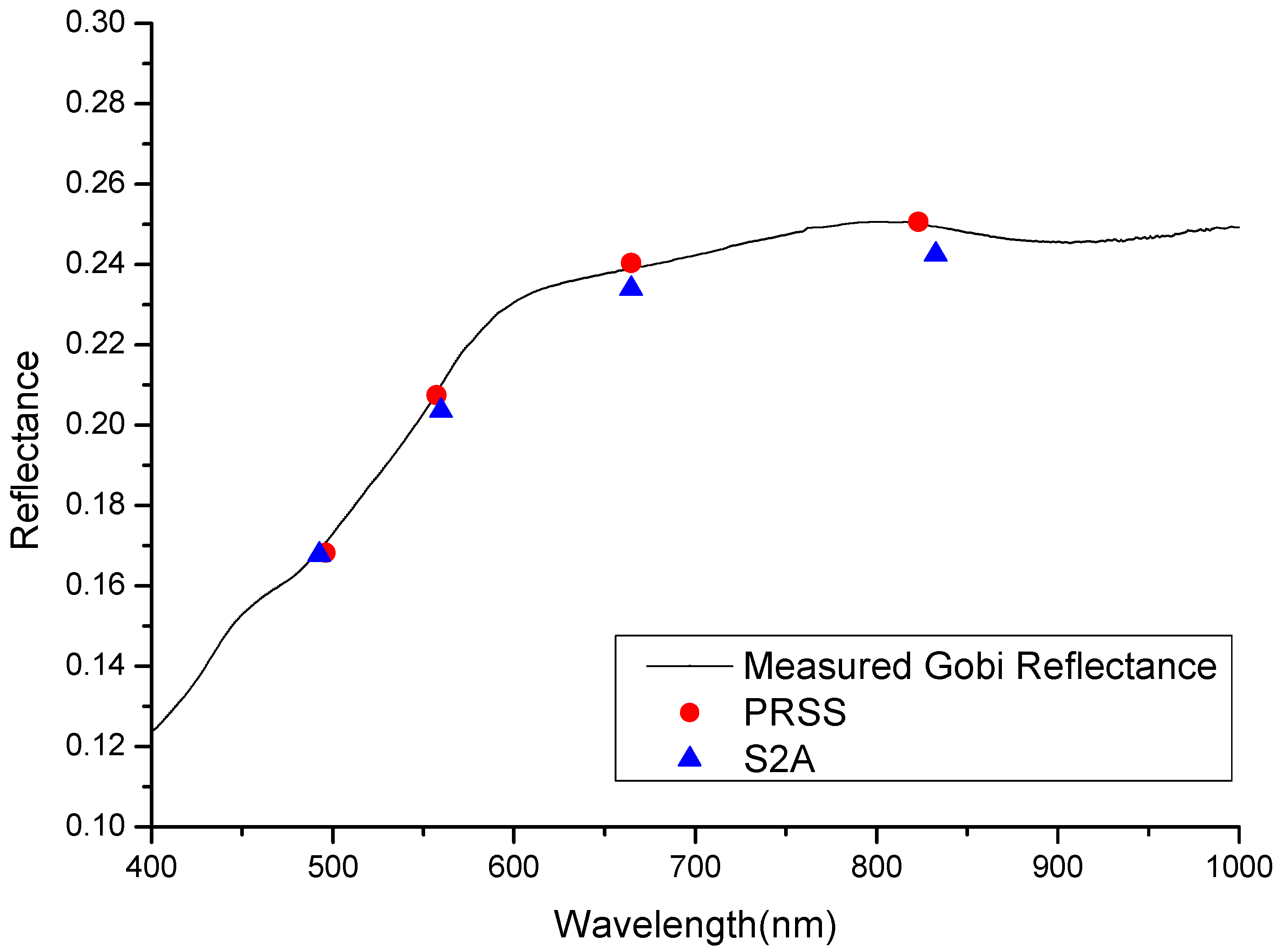
4.2. Reflectance Inversion Verification
5. Discussion
6. Conclusions
Author Contributions
Funding
Data Availability Statement
Acknowledgments
Conflicts of Interest
References
- Yoon, H.; Kacker, R. Guidelines for Radiometric Calibration of Electro-Optical Instruments for Remote Sensing: Handbook (NIST HB); National Institute of Standards and Technology: Gaithersburg, MD, USA, 2015.
- Tan, K.; Wang, X.; Niu, C.; Wang, F.; Du, P.; Sun, D.X.; Yuan, J.; Zhang, J. Vicarious Calibration for the AHSI Instrument of Gaofen-5 With Reference to the CRCS Dunhuang Test Site. IEEE Trans. Geosci. Remote Sens. 2020, 59, 3409–3419. [Google Scholar] [CrossRef]
- Chander, G.; Markham, B.L.; Barsi, J.A. Revised Landsat-5 Thematic Mapper Radiometric Calibration. IEEE Geosci. Remote Sens. Lett. 2007, 4, 490–494. [Google Scholar] [CrossRef]
- Ma, L.; Zhao, Y.; Woolliams, E.R.; Dai, C.; Wang, N.; Liu, Y.; Li, L.; Wang, X.; Gao, C.; Li, C.; et al. Uncertainty Analysis for RadCalNet Instrumented Test Sites Using the Baotou Sites BTCN and BSCN as Examples. Remote Sens. 2020, 12, 1696. [Google Scholar] [CrossRef]
- Bouvet, M.; Thome, K.; Berthelot, B.; Bialek, A.; Czapla-Myers, J.; Fox, N.P.; Goryl, P.; Henry, P.; Ma, L.; Marcq, S.; et al. RadCalNet: A Radiometric Calibration Network for Earth Observing Imagers Operating in the Visible to Shortwave Infrared Spectral Range. Remote Sens. 2019, 11, 2401. [Google Scholar] [CrossRef] [Green Version]
- Pinto, C.T.; Xin, J.; Leigh, L. Evaluation Analysis of Landsat Level-1 and Level2 Data Products Using In Situ Measurements. Remote Sens. 2020, 12, 2597. [Google Scholar] [CrossRef]
- Yeom, J.-M.; Hwang, J.; Jung, J.-H.; Lee, K.-H.; Lee, C.-S. Initial Radiometric Characteristics of KOMPSAT-3A Multispectral Imagery Using the 6S Radiative Transfer Model, Well-Known Radiometric Tarps, and MFRSR Measurements. Remote Sens. 2017, 9, 130. [Google Scholar] [CrossRef] [Green Version]
- Slater, P.N. Radiometric considerations in remote sensing. Proc. IEEE 1985, 73, 997–1011. [Google Scholar] [CrossRef]
- Sun, B.; Schäfer, M.; Ehrlich, A.; Jäkel, E.; Wendisch, M. Influence of atmospheric adjacency effect on top-of-atmosphere radiances and its correction in the retrieval of Lambertian surface reflectivity based on three-dimensional radiative transfer. Remote Sens. Environ. 2021, 263, 112543. [Google Scholar] [CrossRef]
- Ma, L.; Wang, N.; Liu, Y.; Zhao, Y.; Han, Q.; Wang, X.; Woolliams, E.R.; Bouvet, M.; Gao, C.; Li, C.; et al. An In-Flight Radiometric Calibration Method Considering Adjacency Effects for High-Resolution Optical Sensors Over Artificial Targets. IEEE Trans. Geosci. Remote Sens. 2021, 60, 1–13. [Google Scholar] [CrossRef]
- Vermote, E.F.; Tanré, D.; Deuze, J.L.; Herman, M.; Morcette, J.J. Second simulation of a satellite signal in the solar spectrum-vector (6SV). In 6S User Guide Version; IEEE: Piscataway, NJ, USA, 2006; Volume 3, pp. 1–55. [Google Scholar]
- Slater, P.N.; Biggar, S.F.; Thome, K.J.; Gellman, D.I.; Spyak, P.R. Vicarious radiometric calibrations of EOS sensors. J. Atmos. Ocean. Technol. 1996, 13, 349–359. [Google Scholar] [CrossRef] [Green Version]
- Wang, T.; Du, L.; Yi, W.; Hong, J.; Zhang, L.; Zheng, J.; Li, C.; Ma, X.; Zhang, D.; Fang, W.; et al. An adaptive atmospheric correction algorithm for the effective adjacency effect correction of submeter-scale spatial resolution optical satellite images: Application to a WorldView-3 panchromatic image—ScienceDirect. Remote Sens. Environ. 2021, 259, 112412. [Google Scholar] [CrossRef]
- Richter, R. A fast atmospheric correction algorithm applied to Landsat TM images. Int. J. Remote Sens. 1990, 11, 159–166. [Google Scholar] [CrossRef]
- Kaufman, Y.J. Solution of the equation of radiative transfer for remote sensing over nonuniform surface reflectivity. J. Geophys. Res. 1982, 87, 4137–4147. [Google Scholar] [CrossRef]
- Yan, L.; Hongyao, C.; Zhou, F.; Longfei, L.; Yuanwei, C.; Yongli, H.; Hongqiang, W.; Song, W. On-orbit radiometric calibration and accuracy analysis in dual camera of PRSS-1 Satellite. Spacecr. Recovery Remote Sens. 2019, 40, 77–88. [Google Scholar]
- Gascon, F.; Bouzinac, C.; Thépaut, O.; Jung, M.; Francesconi, B.; Louis, J.; Lonjou, V.; Lafrance, B.; Massera, S.; Gaudel-Vacaresse, A.; et al. Copernicus Sentinel-2 Calibration and Products Validation Status. Remote Sens. 2016, 9, 584. [Google Scholar] [CrossRef] [Green Version]
- Lonjou, V.; Lachérade, S.; Fougnie, B.; Gamet, P.; Marcq, S.; Raynaud, J.L.; Tremas, T. Sentinel-2/MSI absolute calibration: First results. In Proceedings of the SPIE Remote Sensing, Toulouse, France, 21–24 September 2015; International Society for Optics and Photonics: Bellingham, WA, USA, 2015. [Google Scholar]
- Angal, A.; Xiong, X.; Shrestha, A. Cross-Calibration of MODIS Reflective Solar Bands with Sentinel 2A/2B MSI Instruments. IEEE Trans. Geosci. Remote Sens. 2020, 58, 5000–5007. [Google Scholar] [CrossRef]


| Measured Reflectance | No Model Used | RCRII Model Used | |||
|---|---|---|---|---|---|
| Inversion Reflectance | Absolute Difference | Inversion Reflectance | Absolute Difference | ||
| Band 1 | 0.599 | 0.591 | 0.00756 | 0.597 | 0.00220 |
| Band 2 | 0.626 | 0.619 | 0.00657 | 0.623 | 0.00224 |
| Band 3 | 0.629 | 0.623 | 0.00654 | 0.626 | 0.00356 |
| Band 4 | 0.606 | 0.598 | 0.00737 | 0.600 | 0.00560 |
| PRSS-1 Band/Sentinel-2A Band | PRSS-1 | Sentinel-2A |
|---|---|---|
| Band1/Band2 | 496.165 | 492.437 |
| Band2/Band3 | 557.375 | 559.849 |
| Band3/Band4 | 664.622 | 664.622 |
| Band4/Band8 | 823.127 | 832.794 |
| PRSS-1 Band/Sentinel-2A Band | Spectral Matching Factor | Relative Deviation (%) | ||
|---|---|---|---|---|
| Band1/Band2 | 1.019 | 101.945 | 101.040 | 0.892 |
| Band2/Band3 | 1.028 | 103.742 | 100.241 | 3.432 |
| Band3/Band4 | 1.038 | 97.504 | 94.385 | 3.251 |
| Band4/Band8 | 1.000 | 67.611 | 65.427 | 3.283 |
| Uncertainty Factors | Relative Uncertainty (%) |
|---|---|
| Calculation of total ground irradiance | 3.0 |
| Target BRDF measurement | 2.0 |
| Calculation of upward transmittance | 2.0 |
| Adjacency effect calculation | 1.0 |
| Others (geometric factors, etc.) | 1.0 |
| Comprehensive uncertainty | 4.4 |
Publisher’s Note: MDPI stays neutral with regard to jurisdictional claims in published maps and institutional affiliations. |
© 2022 by the authors. Licensee MDPI, Basel, Switzerland. This article is an open access article distributed under the terms and conditions of the Creative Commons Attribution (CC BY) license (https://creativecommons.org/licenses/by/4.0/).
Share and Cite
Bao, S.; Chen, H.; Li, Y.; Zhang, L.; Huang, W.; Si, X.; Wang, X.; Fang, Z.; Chen, Y.; Wang, X.; et al. An Improved Vicarious Calibration Method Based on Multi-Grayscale Targets. Remote Sens. 2022, 14, 3779. https://doi.org/10.3390/rs14153779
Bao S, Chen H, Li Y, Zhang L, Huang W, Si X, Wang X, Fang Z, Chen Y, Wang X, et al. An Improved Vicarious Calibration Method Based on Multi-Grayscale Targets. Remote Sensing. 2022; 14(15):3779. https://doi.org/10.3390/rs14153779
Chicago/Turabian StyleBao, Shiwei, Hongyao Chen, Yan Li, Liming Zhang, Wenxin Huang, Xiaolong Si, Xianhua Wang, Zhou Fang, Yuanwei Chen, Xinrong Wang, and et al. 2022. "An Improved Vicarious Calibration Method Based on Multi-Grayscale Targets" Remote Sensing 14, no. 15: 3779. https://doi.org/10.3390/rs14153779
APA StyleBao, S., Chen, H., Li, Y., Zhang, L., Huang, W., Si, X., Wang, X., Fang, Z., Chen, Y., Wang, X., & Zhao, X. (2022). An Improved Vicarious Calibration Method Based on Multi-Grayscale Targets. Remote Sensing, 14(15), 3779. https://doi.org/10.3390/rs14153779