A Quadrifocal Tensor SFM Photogrammetry Positioning and Calibration Technique for HOFS Aerial Sensors

Abstract

Nowadays, the integration between photogrammetry and structure from motion (SFM) has become much closer, and many attempts have been made to combine the two approaches to realize the positioning, calibration, and 3D reconstruction of a large number of images. For the positioning and calibration of high oblique frame sweep (HOFS) aerial cameras, a quadrifocal tensor SFM photogrammetry technique is proposed to resolve the positioning and calibration task of such cameras. It adopts the quadrifocal tensor idea into the OpenMVG SFM pipeline to solve the complexity problem caused by the small single-viewing imaging area and the high image overlapping ratio. It also integrates the photogrammetry iteration idea into the OpenMVG SFM pipeline to enhance the positioning and calibration accuracy, which includes a coarse to fine three-stage Bundle Adjustment (BA) processing approach. In this paper, the overall workflow of the proposed technique was first introduced in detail, from feature extraction and image matching, relative rotation and translation estimation, global rotation and translation estimation, and the quadrifocal tensor model construction to the three-stage BA process and calibration. Then, experiments were carried out in the Zhengzhou area, implementing four types of adjustment methods. The results suggest that the proposed quadrifocal tensor SFM photogrammetry is suitable for large tilt frame sweep camera positioning and calibration without prior information on detailed camera intrinsic parameters and structure. The modifications made to the OpenMVG SFM pipeline enhanced the precision of image positioning and calibration and provided the precision level of professional photogrammetry software.

1. Introduction

Given its high spatial resolution and great flexibility, digital frame cameras are widely used in aerial photogrammetry and remote sensing for topographic mapping, archaeological discoveries, forestry and agricultural assessment, natural disaster monitoring, and ecosystem restoration [1,2,3,4,5,6]. To obtain broader ground coverage, frame digital cameras usually adopt the following technologies: super-wide frame cameras (e.g., Z/I DMC system [4,7]), multi-splicing frame cameras (e.g., Microsoft Ultracam system [4,8], Leica Citymapper system [9], and SWDC-4 cameras [10]), and frame sweep cameras. The representative aerial frame sweep cameras include the EOLOROP [11], DB-110 [12], and VisionMap A3 [13,14,15,16].

Most of these cameras are equipped with Position Orientation System (POS) equipment (including Global Navigation Satellite Systems (GNSS) and Inertial Measurement Units (IMU)) to provide initial camera poses and orientation. Due to significant imaging principles and camera inner structures, the specific camera imagery is always processed through corresponding professional software, such as Ultramap software for Microsoft Ultracam cameras, HxMap software for Leica Citymapper cameras, and LightSpeed for VisionMap A3 cameras [16].

For super-wide and multi-splicing frame cameras, the geometric imaging relationship is relatively simple in nearly vertical photography. Even though the Leica Citymapper camera adopts an oblique photography approach, the angular relationship between different views is fixed. Thus, an accurate geometric imaging model can be established, and high-precision open-source positioning and calibration software can be developed, breaking the limitations of professional software.

In contrast, the frame sweep camera swings along the vertical direction of the flight swiftly for imaging, such as VisionMap A3. It achieves true high-tilt photogrammetry with a long focal length and an ultra-wide sweep angle up to 104 degrees. It can obtain a wide range of clear images at high altitudes, which is particularly useful for surveying, monitoring, and reconnaissance. The obtained multi-angle images are excellent for 3D reconstruction compared to high-resolution satellite images. However, the camera tilt angle varies considerably in dynamic imaging, causing complex geometric imaging relationships and inconsistent imaging scales within one sweep cycle. Moreover, the VisionMap A3 camera is not equipped with an IMU installment, providing no camera orientation information. These increase the difficulty in image positioning processing.

To realize the geometric processing for the VisionMap A3 camera in a more general and simplified way, the research project was implemented, and the performance of the proposed technique was comprehensively analyzed. The rest of the paper is organized as follows. The related works are discussed in the next section, and the VisionMap A3 system is introduced in Section 3. Section 4 presents the methods, including the ideas and workflow. The experimental results and the discussion are provided in Section 5, and a brief conclusion is presented in the last section.

2. Related Work

Photogrammetric techniques have been used to achieve open-source positioning and calibration of the VisionMap A3 camera, but the results have largely been unstable. The main goal of photogrammetry is to generate accurate camera poses (i.e., positions and orientations), intrinsic camera parameters, and 3D points. The processing approach includes matching, aero-triangulation (also called bundle adjustment), orthoimage generation, and digital elevation model (DEM) generation [1,2,3,4,5,17]. Complex geometric imaging relationships and inconsistent imaging scales make it difficult to set up accurate geometric imaging models; thus, many problems occur in processing A3 images by the photogrammetry scheme.

Aside from photogrammetry, SFM has become a common approach in aerial imagery processing. Photogrammetry and SFM approaches have many similarities in feature and bundle adjustment. SFM also computes camera poses, intrinsic parameters, and 3D points cloud [18,19,20]. SFM methods can be categorized into five types: global SFM, incremental SFM, hierarchical SFM, hybrid SFM, and semantic SFM. Global SFM processes all images simultaneously, first solving global camera rotation using the rotation consistency, then calculating camera displacement, and finally applying BA optimization. While the global strategy significantly improves processing efficiency, it is extremely sensitive to external points. Its performance is unstable in many applications, and its reconstruction accuracy is largely unsatisfactory [21,22,23,24,25,26,27,28].

Incremental SFM starts with two or three view reconstructions, gradually adds new views, and then applies BA operation after each addition. This processing method is robust with high reconstruction accuracy, and most popular SFM pipelines employ incremental approaches. However, incremental SFM has drift risk due to the accumulation of errors [29,30,31,32,33,34,35,36,37]. Hierarchical SFM is the revision of the traditional incremental SFM. It divides the large-scale datasets into N interrelated sub-datasets, and then parallel incremental SFM processing is performed on the sub-datasets. Finally, the sub-datasets are merged [38,39,40,41]. Hybrid SFM combines the advantages of global SFM and incremental SFM. It solves camera rotation using the global approach and then calculates camera displacement incrementally [42,43,44]. Semantic SFM uses the semantic label to detect the corresponding models and facilitate image matching and camera calibration. Scene segmentation can be realized in SFM reconstruction [45,46,47].

The well-known SFM pipelines include Bundler [31,32], VisualSFM [35], COLMAP [34,37], and OpenMVG [29,36]. The properties of these pipelines are summarized in

Table 1. Popular SFM Pipelines Analysis.

Pipeline	Properties
Bundler	An early incremental SFM pipeline originated from Photo Tourism Project. The time complexity is O(n4), the output is sparse point clouds, and the operation is complex.
VisualSFM	A revision on Bundler and the time complexity reaches O(n1), the output is dense point clouds with higher accuracy, and the operation is much simpler.
COLMAP	COLMAP improves scene graph verification, next best view selection, sampling-based triangulation, and bundle adjustment; it performs better in terms of completeness and robustness. Its efficiency outperforms OpenMVG but does not support POS data input.
OpenMVG	OpenMVG adds an efficient contrario trifocal tensor estimation method and translation registration technique into the original SFM pipeline. It outperforms many incremental and global pipelines in terms of accuracy and running times. The reprojection error and the drift are smaller than COLMAP, and it supports POS data input.

Notes: n is the number of images.

.

At present, the integration between photogrammetry and SFM has become more pronounced. SFM photogrammetry combines the two approaches to realize the positioning, calibration, and 3D reconstruction of a large number of ordered and disordered images [48].

Photogrammetry often relies on initial POS data and intrinsic camera parameters and can reach higher accuracy through iterative least-squares adjustment, condition adjustment, or indirect adjustment. SFM takes homogeneous coordinates in expression and does not require specific initial values of POS data and intrinsic camera parameters. In image pose recovery and 3D reconstruction, SFM uses the R matrix to model the attitude angle system, which does not involve selecting a specific angle rotation system; thus, it can overcome challenges caused by the swift change of the sweep angle in the ultra-wide imaging range. It also avoids conversion among different coordinate systems, resulting in much simpler operations and faster convergence. Thus, the SFM pipeline was chosen to solve the positioning and calibration task of the VisionMap A3 camera.

By analyzing Table 1 it can be determined that the OpenMVG pipeline has smaller reprojection and drift errors and supports POS data input, which is especially advantageous for remote sensing imagery. Thus, the OpenMVG pipeline was chosen for the geometric processing of VisionMap A3 images, addressing the limitations of the professional LightSpeed software.

Wu et al. [35] introduced a novel BA strategy that provides a good balance between SFM reconstruction speed and accuracy and maintains high accuracy by regularly re-triangulating feature matches that fail to triangulate. Wu’s feature detection and description algorithm was adopted into the OpenMVG pipeline. Moulon et al. [36] proposed a new global calibration approach based on the fusion of relative motions between image pairs, presenting an efficient contrario trifocal tensor estimation method and translation registration technique for accurate camera positions recovery in OpenMVG. We followed the tensor cluster idea and designed the quadrifocal tensor-based BA method.

Two main improvements were introduced to the original OpenMVG pipeline. First, the VisionMap A3 frame sweep camera has a small single-viewing imaging area. The high image overlapping ratio and the high number of images enhance the processing complexity. To reduce the complexity and strengthen the robustness, the quadrifocal tensor was added to the OpenMVG pipeline, which deals with the images in the quadrifocal tensor model cluster. The quadrifocal tensor model performs high oblique frame sweep camera positioning and calibration processing as an independent unit. Second, the photogrammetry iteration idea was introduced into the OpenMVG pipeline to enhance the positioning and calibration accuracy. A coarse to fine three-stage BA processing approach was proposed to deal with the pose parameters and the intrinsic parameters.

The quadrifocal tensor-based positioning and calibration method first carries out feature extraction and image matching. Relative rotation and translation estimation and global rotation and translation are performed before establishing the quadrifocal tensor model. The three-dimensional coordinates of matching points in each quadrifocal tensor model are calculated, and the BA cost function is finally set up with the quadrifocal tensor model as the independent unit. Real VisionMap A3 data is then used to evaluate whether the proposed approach can solve the high oblique frame sweep camera position and calibration problem in a more general and simplified way.

3. VisionMap A3 System Introduction

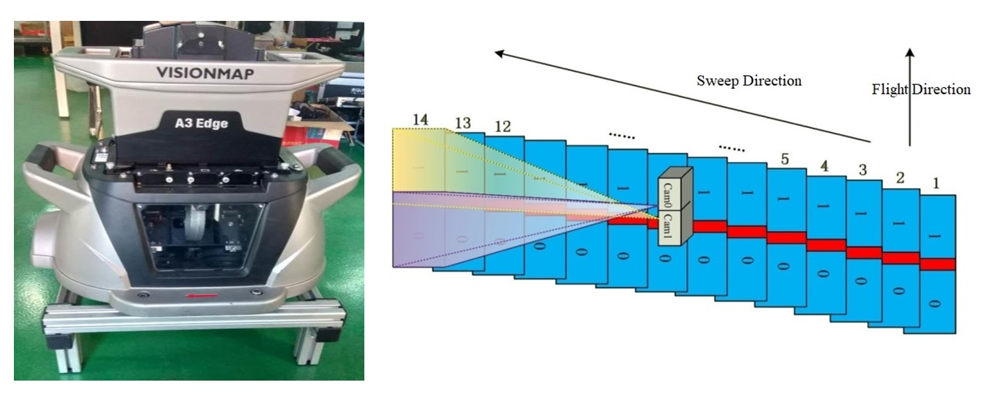
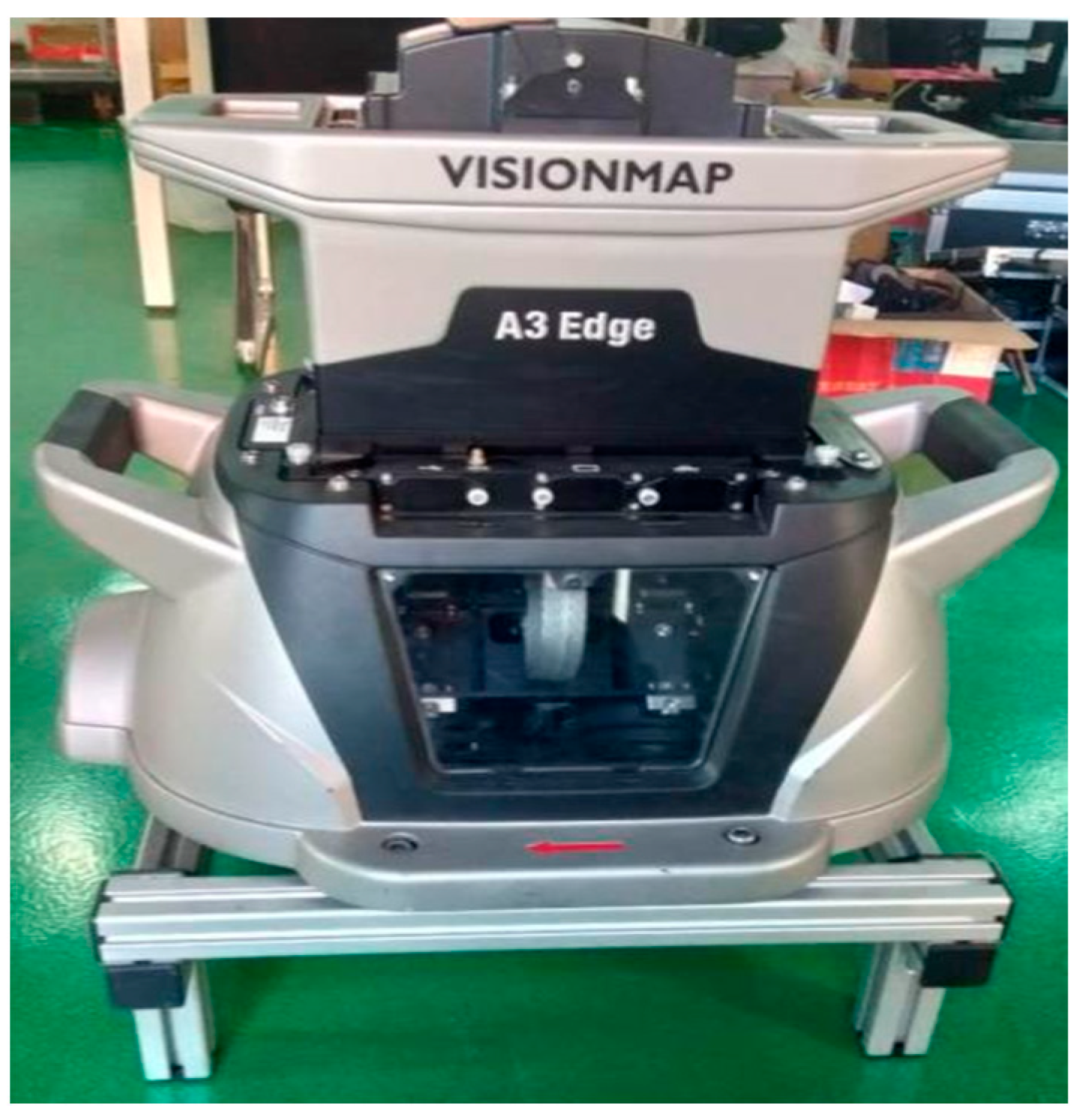
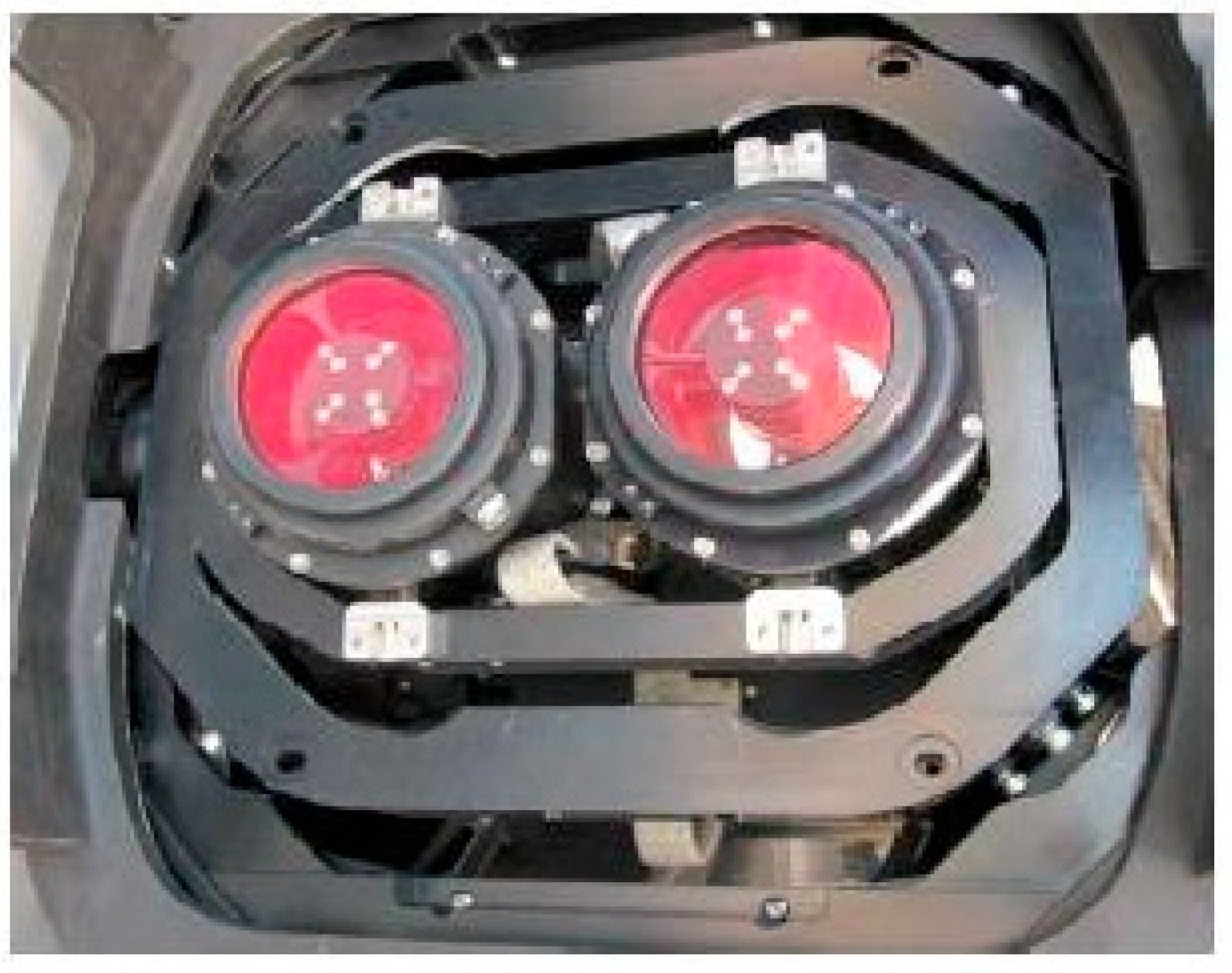
The VisionMap A3 system is a fully automated mapping system established in 2004. The system consists of an airborne digital step-framing double lens metric camera and a ground processing system. The airborne system consists of dual CCDs with two 300 mm lenses (Figure 1 and Figure 2), a fast compression and storage unit, and a dual-frequency GPS. The long focal length yields comparatively high ground resolution when flying at high altitudes, enabling efficient photography of large areas in high resolution.

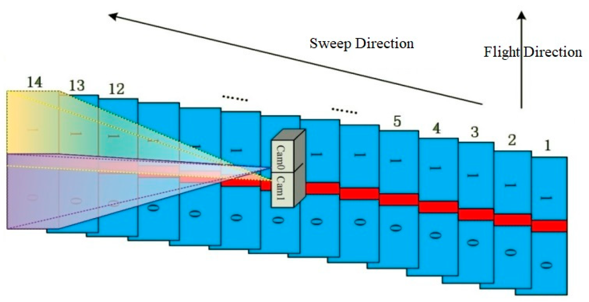
During the flight, a sequence of frames is exposed in a cross-track direction at a very high speed to provide a very wide angular coverage of the ground. The two lenses of the camera simultaneously sweep across the flight direction from one side to the opposite side, with each CCD capturing about 27 frames (54 frames for two CCDs) and having a maximum sweep angle of 104 degrees. After completing the first sweep, the lenses return to the start position in preparation for the next sweep. The sweep back time is 0.5 s. Each CCD captures seven frames per second (one frame in 0.142 s); therefore, a single sweep is completed in approximately 3.6 s. The time between sweeps depends largely on the aircraft speed, flight altitude, and the required overlap between two consecutive sweeps. For more details on the technical parameters, refer to Pechatnikov et al. [13].

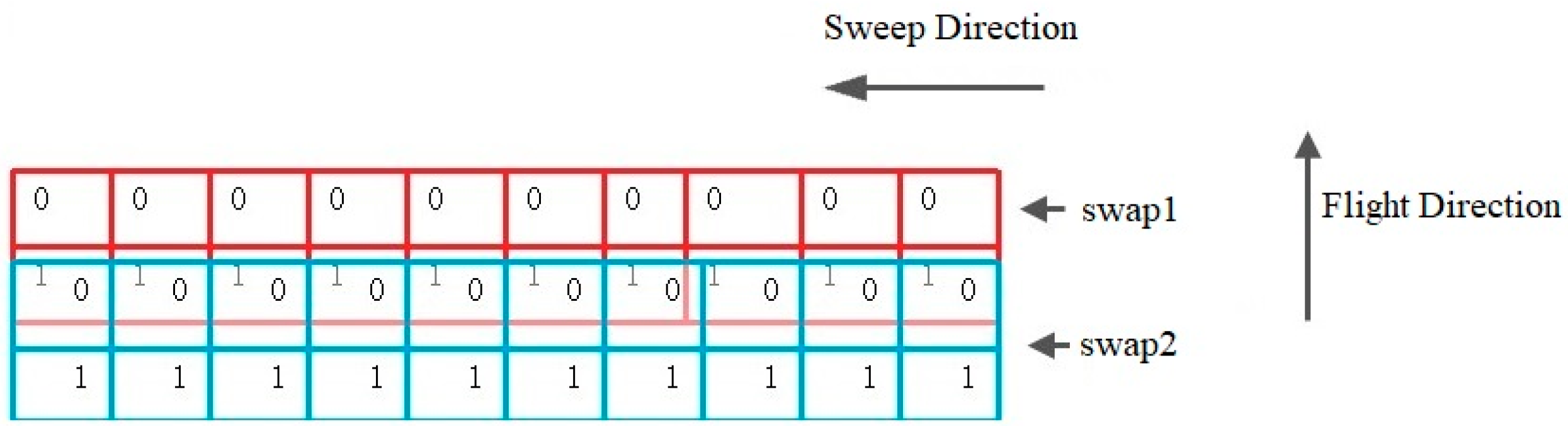
Two adjacent single frames along the flight form a double frame (Figure 3 and Figure 4). The overlap between two adjacent single frames is about 2% (~100 pix), while the overlap between two adjacent double frames across the flight direction is about 15%. The overlap between two consecutive sweeps along the flight direction is typically 56%, but this value may vary depending on the defined specifications of the aerial survey. Between two consecutive flight lines, the overlap is generally 50% to enable stereo photogrammetric mapping. All overlaps are determined during flight planning and may be altered during the flight. VisionMap A3 camera provides orthogonal coverage of the nadir area and oblique coverage of the remainder of the sweep image. As all images participate in all stages of the analytical computations, after performing matching and block adjustment, accurate solutions for all images, including the oblique images, can be obtained. The generation of accurately solved oblique images simultaneously with regular verticals is a unique and highly important feature of the A3 system.

4. The Proposed Quadrifocal Tensor SFM Photogrammetry Positioning and Calibration Technique

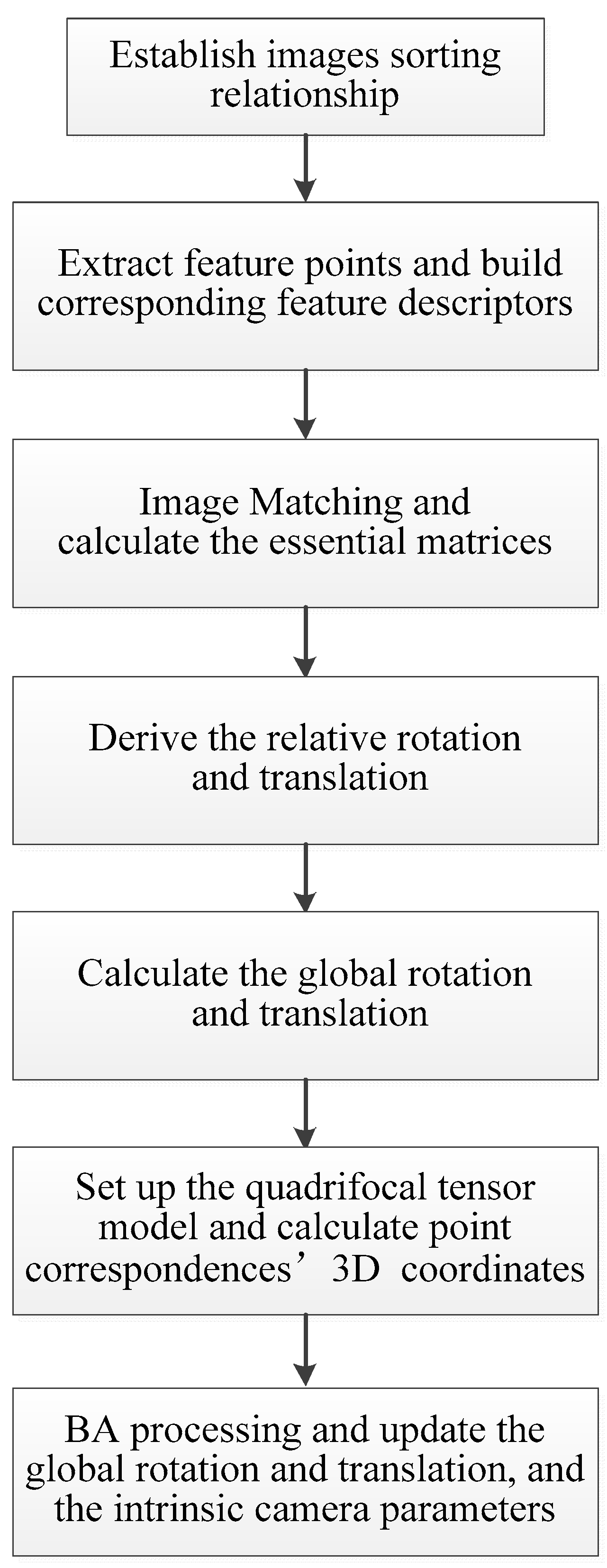
The proposed quadrifocal tensor SFM photogrammetry positioning and calibration technique include the following steps. First, all aerial images are sorted by flight route according to imaging time, and the sorting relationship is established. The scale-invariant feature transform (SIFT) algorithm is then used to extract feature points on each view and build corresponding feature descriptors according to the image sorting relationship. The iterative feature matching process is then carried out under the Hamming distance criterion. The RANSAC algorithm is used to eliminate mismatches in the matching results, and the feature point correspondences on the pairwise overlapping images are determined. The pinhole imaging model is then established based on the unknown camera geometric distortion parameters, and the essential matrices between each pairwise overlapping view are calculated using the successful matching point correspondences and redundant constraints. The relative spatial rotation and the translation relationship, i.e., the rotation matrix R and the translation vector t, are derived from the essential matrices.

After performing the Bayesian inferences, the initial global rotations are computed for each view in a global coordinate system, while the initial global translations are generated using the initial POS data or from the translation registration. The quadrifocal tensor model can then be established, and the initial three-dimensional coordinates of the matching point correspondences in each quadrifocal tensor model are calculated. Finally, the BA cost function based on the quadrifocal tensor model is constructed and used in the BA processing. The global rotation matrix and the translation vector for each view are updated, and the intrinsic parameters are calibrated simultaneously. The general workflow is listed in Figure 5.

4.1. Feature Extraction and Image Matching

The SIFT algorithm is used to extract the feature points on each view and build corresponding feature descriptors simultaneously according to the image sorting relationship [49]. The Hamming distance is taken as the criterion for iterative image matching, and the RANSAC algorithm is adopted to eliminate a large number of mismatches in the matching results.

4.2. Relative Rotation and Translation Estimation

The pinhole camera model is used to describe the frame sweep aerial camera. The three-dimensional point P(X, Y, Z) in the ground object space is projected onto the image plane and forms an image point p(x, y, −f) through the pinhole projection. The geometric relationship between the object point and the image point can be described with the following model:

$$\mathrm{x}=\mathrm{PX}=\mathrm{K}\left[\left.\mathrm{R}\right|\mathrm{t}\right]\mathrm{X}$$

(1)

where R is the rotation matrix, a 3 × 3 orientation matrix representing the direction of the camera coordinate system; t is the position vector; R and t are the camera exterior parameters; K is the camera intrinsic parameter matrix (also called the camera calibration matrix). The frame sweep camera positioning and calibration determine the R, t, and K matrices; the camera projection matrix is provided by P = K[R|t].

The general form of the calibration matrix for a CCD camera is:

$$\mathrm{K}=\left[\begin{array}{ccc}{\alpha }_x& & x_0\\ & {\alpha }_y& y_0\\ & & 1\end{array}\right].$$

(2)

To increase generality, the skew parameter s can be added,

$$\mathrm{K}=\left[\begin{array}{ccc}{\alpha }_x& s& x_0\\ & {\alpha }_y& y_0\\ & & 1\end{array}\right].$$

(3)

Based on the successful matching point correspondences obtained in Section 4.1, the relative spatial rotation and translation between any two overlapping images can be calculated. The pairwise point correspondence p₁, p₂ meets the following epipolar constraint:

$$p_2^{\mathrm{T}}{\mathrm{K}}^{-\mathrm{T}}{\mathrm{EK}}^{-1}{p}_1=0$$

(4)

In Equation (4), the points O₁, P, and O₂ are coplanar. E is the essential matrix, which is the outer product of t and R and is perpendicular to t and R. Both translation and rotation are included in the epipolar plane constraint, and the essential matrix E is calculated from the point correspondences. After obtaining the essential matrix E, singular value decomposition (SVD) is performed on the matrix E matrix to obtain R. Thus, the relative rotation and translation of the two overlapping images can be determined [18,29,36].

4.3. Global Rotation and Translation Estimation

Assuming that in the global coordinate system, the global rotation matrix of image i is R_i, that of image j is R_j, and the relative rotation is R_ij, which is obtained in Section 4.2. Three rotation matrices meet the consistency Equation (5), which is the basis for solving the global rotation.

$${\mathrm{R}}_j={\mathrm{R}}_{ij}{\mathrm{R}}_i.$$

(5)

R_j is orthonormal, for j = 1, …, m.

While the RANSAC algorithm can remove most mismatches, there are remaining mismatches that cause deviations in the relative rotation estimation. As relative R_ij estimates may contain outliers, the global rotation estimation must be robust in identifying the global rotations and the inconsistent/outlier edges (false essential geometry). Moulon’s method [36] is used in determining inconsistent relative rotations in Bayesian inference. The iterative use of the Bayesian inference, adjusted with the cycle length weighting, can remove most outliers, check all the triplets of the graph, and reject those with cycle deviations larger than 2°.

When the relative rotations are known, they form a tree graph with the views as vertices connected by an edge. Equation (5) can be solved by least-squares while satisfying the orthonormality conditions, R can be expressed in quaternions [50], and Equation (5) is transformed into

$${\dot{r}}^j={\dot{r}}^{ij}{\dot{r}}^i$$

(6)

where ${\dot{r}}^j$ and ${\dot{r}}^i$ are the unknown quaternions of the ith and jth view rotation, respectively, and ${\dot{r}}^{ij}$ is the known relative rotation between views i and j. Each quaternion can be considered a four-vector. Using known manipulations with quaternions, each equation in (6) can be rewritten as

$$\left(\begin{array}{c}{r}_0^j\\ r_x^j\\ r_y^j\\ r_z^j\end{array}\right)=\left[\begin{array}{cccc}{r}_0& -r_x& -r_y& -r_z\\ r_x& r_0& -r_z& r_y\\ r_y& r_z& r_0& -r_x\\ r_z& -r_y& r_x& r_0\end{array}\right]\left(\begin{array}{c}{r}_0^i\\ r_x^i\\ r_y^i\\ r_z^i\end{array}\right)$$

(7)

where ${\dot{r}}^i=r_0^i+i{r}_x^i+j{r}_y^i+k{r}_z^i$, with i, j, and k as imaginary units. There are 4m unknowns $r_0^1,r_x^1,r_y^1,r_z^1,\cdots ,r_0^m,r_x^m,r_y^m,r_z^m$ with constraints (7) for each view pair ij with a known rotation. After the solution, the quaternions can be easily made into units by dividing each by its Euclidean length.

After deciding on the global rotations, the next step is determining the global translations. Given a set of relative motion pairs (R_ij, t_ij) (rotations and translation directions solved in Section 4.2), the global location $\left(T_1,\cdots ,T_m\right)$ of all views can be obtained. The different translation directions are reconciled in the global coordinates system.

$$‖T_j-R_{ij}{T}_i-{\lambda }_{ij}{t}_{ij}‖=0,\begin{array}{cc}& \end{array}\forall i,j$$

(8)

To solve m global translations and scale factors ${\lambda }_{ij}$, the solution for Equation (7) is optimized using the least-squares method or Moulon’s approach [36] under the $l_{\infty }$ norm. For the VisionMap A3 edge camera, the GPS equipment provides the camera with position information in the world coordinate system, so the processed GPS information can be taken as initial values $\left(T_1,\cdots ,T_m\right)$.

4.4. Set up the Quadrifocal Tensor Model and Calculate Initial 3D Ground Point

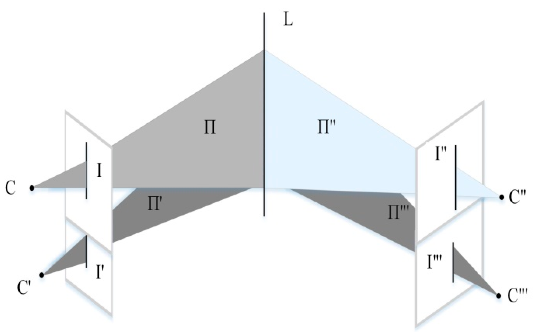
Subsequently, the quadrifocal tensor model would be established, and the global translations and three-dimensional coordinates of the point correspondences would then be determined based on the quadrifocal tensor model. For the VisionMap camera, at a certain sweep angle, the cam0 and cam1 lenses obtain images I and I′, the corresponding projection planes are II and II′, and the projection centers are C and C′. The sweep angle changes swiftly. At the next imaging moment, the cam0 and cam1 lenses obtain images I″ and I‴, with the corresponding projection planes II″ and II‴ and projection centers C″ and C‴. The straight line L in the object space is reflected on four image views (see Figure 6).

When the camera projection matrices of the four image views are A, B, C, and D, a three-dimensional ground point X projects onto the four image views, and there is a set of corresponding points $\mathrm{x}\leftrightarrow \mathrm{x}\prime \leftrightarrow \mathrm{x}″\leftrightarrow \mathrm{x}‴$ across the four views. The four image views constitute a quadrifocal tensor model, and the projection relationship among the four views is provided by:

$$\left[\begin{array}{ccccc}\mathrm{A}& \mathrm{x}& & & \\ \mathrm{B}& & \mathrm{x}\prime & & \\ \mathrm{C}& & & \mathrm{x}″& \\ \mathrm{D}& & & & \mathrm{x}‴\end{array}\right]\left[\begin{array}{c}\mathrm{X}\\ -k\\ -k^{\prime }\\ -k^{″}\\ -k^{‴}\end{array}\right]=0$$

(9)

where $k$, $k^{\prime }$, $k^{″}$, and $k^{‴}$ represent uncertain scale constants, and ${\mathrm{a}}^i$, ${\mathrm{b}}^i$, ${\mathrm{c}}^i$, and ${\mathrm{d}}^i$ are the row vectors of matrices A, B, C and D, respectively. The rank-4 tensor ${\mathrm{Q}}^{pqrs}$ is defined by

$${\mathrm{Q}}^{pqrs}=\det \left[\begin{array}{c}{\mathrm{a}}^i\\ {\mathrm{b}}^q\\ {\mathrm{c}}^r\\ {\mathrm{d}}^s\end{array}\right].$$

(10)

From Equation (9), the quadrilinear relationship can be derived in the following form for the quadrifocal tensor:

$$x^i{x^{\prime }}^j{x^{″}}^k{x^{‴}}^l{\epsilon }_{ipw}{\epsilon }_{jqx}{\epsilon }_{kry}{\epsilon }_{lsz}{\mathrm{Q}}^{pqrs}=0_{wxyz}$$

(11)

where $0_{wxyz}$ is a zero tensor with four indices $w,x,y$ and $z$; ${\epsilon }_{ipw}$,${\epsilon }_{jqx}$,${\epsilon }_{kry}$ and ${\epsilon }_{lsz}$ represent the product between the different vectors. Based on the global rotation and translation computed in Section 4.3, the camera projection matrices A, B, C, and D are determined, and the quadrifocal tensor model can then be established.

The next step is realizing 3D reconstruction for point correspondences in the quadrifocal tensor model. The ground point X projects across four views and forms the corresponding image points $\mathrm{x}\leftrightarrow \mathrm{x}\prime \leftrightarrow \mathrm{x}″\leftrightarrow \mathrm{x}‴$. The geometric projection relationship between the ground point and the corresponding image point is listed as follows:

$$\left\{\begin{array}{c}\mathrm{x}=\mathrm{AX}\\ \mathrm{x}\prime =\mathrm{BX}\\ \mathrm{x}″=\mathrm{CX}\\ \mathrm{x}‴=\mathrm{DX}\end{array}\right.$$

(12)

The plane coordinate of the image point $\mathrm{x}$ is (x, y). Taking the first expression in Equation (12) as an example, when the cross product is applied, and the homogeneous scalar factor is eliminated, the following equations can be obtained:

$$\left\{\begin{array}{c}x{(\mathrm{A}}^{3\mathrm{T}}\mathrm{X})-\left({\mathrm{A}}^{1\mathrm{T}}\mathrm{X}\right)=0\\ y{(\mathrm{A}}^{3\mathrm{T}}\mathrm{X})-\left({\mathrm{A}}^{2\mathrm{T}}\mathrm{X}\right)=0\\ x{(\mathrm{A}}^{2\mathrm{T}}\mathrm{X})-y\left({\mathrm{A}}^{1\mathrm{T}}\mathrm{X}\right)=0\end{array}\right..$$

(13)

Taking the first two equations, which are linearly independent, the four image points $\mathrm{x}\leftrightarrow \mathrm{x}\prime \leftrightarrow \mathrm{x}″\leftrightarrow \mathrm{x}‴$ develop into eight equations

$$\begin{gathered} \mathrm{NX}-\mathrm{L}=0 \\ \mathrm{N}=\left[\begin{array}{c}x{\mathrm{A}}^{3\mathrm{T}}-{\mathrm{A}}^{1\mathrm{T}}\\ y{\mathrm{A}}^{3\mathrm{T}}-{\mathrm{A}}^{2\mathrm{T}}\\ x^{\prime }{\mathrm{B}}^{3\mathrm{T}}-{\mathrm{B}}^{1\mathrm{T}}\\ y^{\prime }{\mathrm{B}}^{3\mathrm{T}}-{\mathrm{B}}^{2\mathrm{T}}\\ x^{″}{\mathrm{C}}^{3\mathrm{T}}-{\mathrm{C}}^{1\mathrm{T}}\\ y^{″}{\mathrm{C}}^{3\mathrm{T}}-{\mathrm{C}}^{2\mathrm{T}}\\ x^{‴}{\mathrm{D}}^{3\mathrm{T}}-{\mathrm{D}}^{1\mathrm{T}}\\ y^{‴}{\mathrm{D}}^{3\mathrm{T}}-{\mathrm{D}}^{2\mathrm{T}}\end{array}\right]. \end{gathered}$$

(14)

Solving Equation (14) by the least-squares approach, the 3D coordinates for ground point X are generated.

4.5. Bundle Adjustment Based on the Quadrifocal Tensor Model

The BA processing is performed to update the rotation and translation and simultaneously calibrate the intrinsic matrix. The BA cost function based on the quadrifocal tensor model is defined in the form as

$$f\left(z\right)=‖\left(x_i-\frac{{\mathrm{R}}_i^1{\mathrm{X}+\mathrm{t}}_i^1}{{\mathrm{R}}_i^3{\mathrm{X}+\mathrm{t}}_i^3},y_i-\frac{{\mathrm{R}}_i^2{\mathrm{X}+\mathrm{t}}_i^2}{{\mathrm{R}}_i^3{\mathrm{X}+\mathrm{t}}_i^3}\right)‖$$

(15)

where $\left(x_i,y_i\right),i\in \left(1,2,3,4\right)$ is the observation value corresponding to the four image points $\mathrm{x}\leftrightarrow \mathrm{x}\prime \leftrightarrow \mathrm{x}″\leftrightarrow \mathrm{x}‴$; ${\mathrm{R}}_i,i\in \left(1,2,3,4\right)$ is the corresponding rotation matrix to each view; ${\mathrm{t}}_i,i\in \left(1,2,3,4\right)$ is the corresponding translation vector; $\left(\frac{{\mathrm{R}}_i^1{\mathrm{X}+\mathrm{t}}_i^1}{{\mathrm{R}}_i^3{\mathrm{X}+\mathrm{t}}_i^3},\frac{{\mathrm{R}}_i^2{\mathrm{X}+\mathrm{t}}_i^2}{{\mathrm{R}}_i^3{\mathrm{X}+\mathrm{t}}_i^3}\right)$ is the calculation value of the image point; z is the unknown parameter vector comprising the camera pose and calibration parameters (i.e., unknowns in rotation and translation) and the 3D ground point coordinates X.

The differences between the observed values and the calculation values of the image points are the reprojection error of the ground point, representing the errors contained in the rotation, translation, and camera calibration parameters and the ground point coordinates. When the cost function reaches the minimum value, the optimal solution is obtained for the pose parameters, calibration parameters, and 3D coordinates of ground points.

The BA process optimizes the following nonlinear least-squares BA cost function

$$z^{\ast }=\arg \min {\displaystyle \sum _{k=1}^n{‖f_k\left(z\right)‖}^2}.$$

(16)

The BA cost function is optimized by the Levenberg–Marquardt (LM) approach. The LM algorithm decomposes the original nonlinear cost function (Equation (16)) into approximations of a series of regularized linear functions and $J\left(z\right)$ is the Jacobian matrix of $f\left(z\right)$. In each loop, the LM approach updates the linear least squares problem in the following form:

$${\delta }^{\ast }=\arg \underset{\delta }{\min }{‖J\left(z\right)\delta +f\left(z\right)‖}^2+\lambda ‖D\left(z\right)\delta ‖.$$

(17)

If $‖f\left(z+{\delta }^{\ast }\right)‖<‖f\left(z\right)‖$, then the unknown parameter is updated as $z\to z+{\delta }^{\ast }$. $D\left(z\right)$ is the square root matrix of the matrix $J{\left(z\right)}^{\mathrm{T}}J\left(z\right)$ and $\lambda$ is the regularization parameter, which can be adjusted according to the approximation between $J\left(z\right)$ and $f\left(z\right)$. Solving Equation (17) is equivalent to solving the standard equation:

$$\left(J^{\mathrm{T}}J+\lambda D^{\mathrm{T}}D\right)\delta =-J^{\mathrm{T}}f$$

(18)

where $\left(J^{\mathrm{T}}J+\lambda D^{\mathrm{T}}D\right)$ is the extended Hessian matrix. In the BA process, the unknown parameter $z$ includes two parts: the camera pose and calibration parameters ($z_c$) and the 3D ground point coordinates ($z_p$). Similarly, $D,\delta ,J$ can also be divided into two parts. Let $U=J_c^{\mathrm{T}}{J}_c$, $V=J_p^{\mathrm{T}}{J}_p$, $U_{\lambda }=U+\lambda D_c^{\mathrm{T}}{D}_c$, $V_{\lambda }=V+\lambda D_p^{\mathrm{T}}{D}_p$, $W=J_c^{\mathrm{T}}{J}_p$; Equation (18) can then be rewritten as the block structure linear system:

$$\left[\begin{array}{cc}{U}_{\lambda }& W\\ W^{\mathrm{T}}& V_{\lambda }\end{array}\right]\left[\begin{array}{c}{\delta }_c\\ {\delta }_p\end{array}\right]=-\left[\begin{array}{c}{J}_c^{\mathrm{T}}f\\ J_p^{\mathrm{T}}f\end{array}\right].$$

(19)

Applying the Gaussian elimination method to Equation (19), the 3D coordinates of the ground points can be eliminated, and a linear equation containing just the camera pose and calibration parameters can be obtained:

$$\left(U_{\lambda }-W{V}_{\lambda }^{-1}{W}^{\mathrm{T}}\right){\delta }_c=-J_c^{\mathrm{T}}f+W{V}_{\lambda }^{-1}{J}_p^{\mathrm{T}}f.$$

(20)

Therefore, ${\delta }_c$ can be determined by solving Equation (20) and ${\delta }_p$ can then be solved by reverse substitution.

$${\delta }_p=-V_{\lambda }^{-1}\left(J_p^{\mathrm{T}}f+W^{\mathrm{T}}{\delta }_c\right).$$

(21)

The variables ${\delta }_c$ and ${\delta }_p$ are obtained using an iterative solution; after two loops, both can reach high precision. The quadrifocal tensor SFM positioning and calibration process for the frame sweep aerial camera is therefore completed.

To obtain better positioning and calibration precision, the OpenMVG SFM pipeline is improved according to the photogrammetry processing mode. In photogrammetric processing, position deviation is mostly caused by pose errors, while the intrinsic camera parameters generate minor systematic errors for both aerial and satellite-borne cameras [51,52]. So in the photogrammetry BA implementation, BA is always carried out in several stages. Pose parameters are dealt with first, while the intrinsic parameters are processed last. Here, three-stage BA processing is put forward. In the first stage, the intrinsic matrix K is set to E (identity matrix), the rotation R remains unchanged, and only the translation T and the 3D coordinates of ground points X are involved. In the second stage, the intrinsic matrix K remains as E, but the translation T, the rotation T, and the 3D coordinates of ground points X are involved in the BA process. In the last stage, all the unknowns, the intrinsic parameter K, the translation T, the rotation T, and the 3D coordinates of ground points X are adjusted.

5. Experiments and Analysis

5.1. Test Data

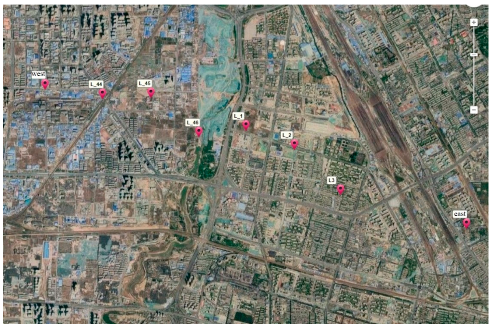
The VisionMap Edge A3 camera was used to photograph the Zhengzhou area in January 2020, with a total flight area of about 1000 square kilometers. Two flight missions were carried out at 2300 m flight altitude, generating a ground resolution of about 5 cm. Six routes (L_44, L_45, L_46, L_1, L_2, and L_3), located in the middle region and covering about 120 square kilometers, were used for the experiment (see Figure 7).

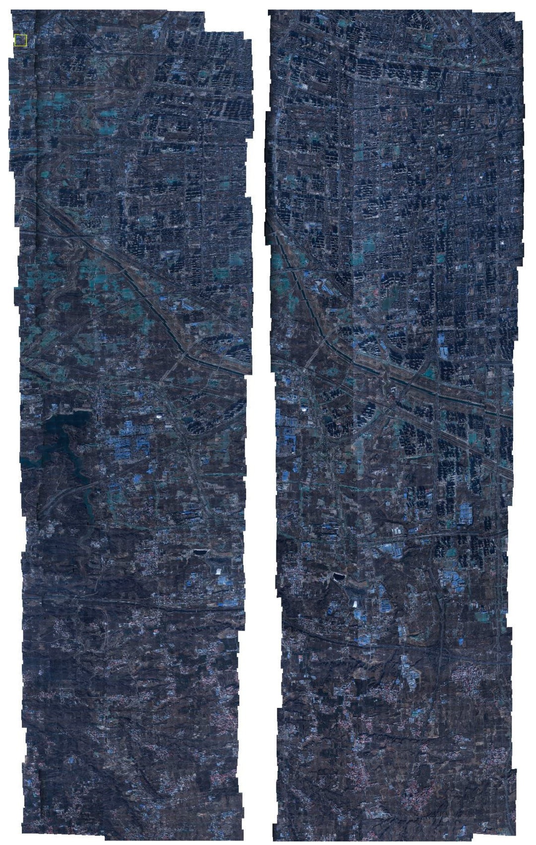
The upper half is selected for analysis, comprising 7928 images and covering a total area of 64 square kilometers. The study area (shown in Figure 8) includes plain regions and urban areas.

Four different calibration approaches were designed to evaluate and compare the proposed quadrifocal tensor SFM photogrammetry method with the original OpenMVG SFM pipeline. The proposed method is tested under different conditions: no Ground Control Point (GCP) support, with GCP support without considering camera intrinsic parameters, and with GCP support considering camera intrinsic parameters.

I.

The proposed method with no GCP support

The whole procedure in Figure 5 was implemented using POS. All unknowns, rotation, translation, intrinsic parameters, and 3D ground point coordinates were involved in this process.

II.

The proposed method with GCP support, but not considering camera intrinsic parameters

The proposed method with GCP support was evaluated. All the unknowns were employed in the BA procedure except the intrinsic camera parameters. The whole flow was similar to the first test, but the intrinsic parameter matrix remained an identity matrix.

III.

The proposed method with GCP support and considering camera intrinsic parameters

The same group of GCPs takes part in the test. All the unknowns, including the intrinsic parameters, are involved in the BA procedure. The intrinsic parameter model adopted Model (4), and the variables ${\alpha }_x$ and ${\alpha }_y$ each absorbed two distortion parameters. In the adjustment process, the weight value of the ground control points was 20 times that of the point correspondences.

• IV. The original OpenMVG SFM pipeline with GCP support

The same group of GCPs and checkpoints (CHK) was used to evaluate the performance of the original OpenMVG pipeline.

5.2. The Proposed Method with No GCP Support

A total of 7916 images were used in the experiment, and 6,856,633 pairwise point correspondences were extracted from matching. Thirteen ground CHKs were used to measure the discrepancies (i.e., ground point residuals) between the 3D observation values and the calculated estimates. The statistical results of residuals are shown in

Table 2. Statistical Values for CHKs after the First Experiment (Unit: meter).

ID of CHK	X-Axis	Y-Axis	Z-Axis
CHK 1	0.7285	−0.7146	−17.6891
CHK 2	1.3723	−0.5638	−19.4138
CHK 3	0.2392	−0.5449	−16.8526
CHK 4	0.5169	−0.1780	−17.2758
CHK 5	0.2371	−0.5560	−16.6415
CHK 6	−0.0221	−0.3999	−16.5177
CHK 7	1.0317	0.5181	−16.6787
CHK 8	0.6388	0.8845	−16.2159
CHK 9	−1.8655	0.4107	−17.0058
CHK 10	−0.2723	0.1838	−16.7048
CHK 11	0.0234	0.8457	−16.6783
CHK 12	−0.2252	1.3395	−17.2606
CHK 13	−0.6135	0.9441	−17.7322
RMSE	0.7966	0.6950	17.14631

, and the root mean squares error (RMSE) is presented in the last row.

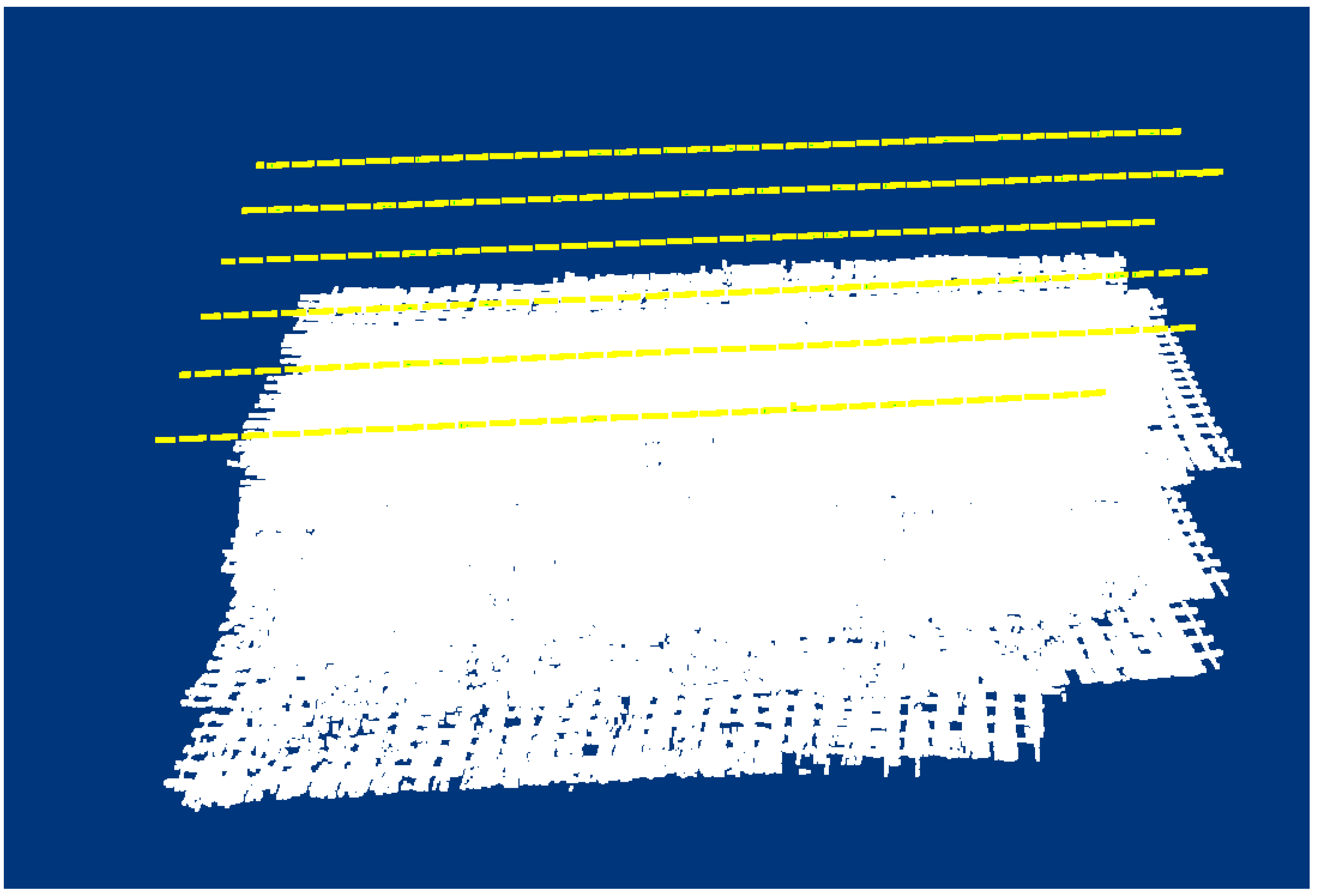
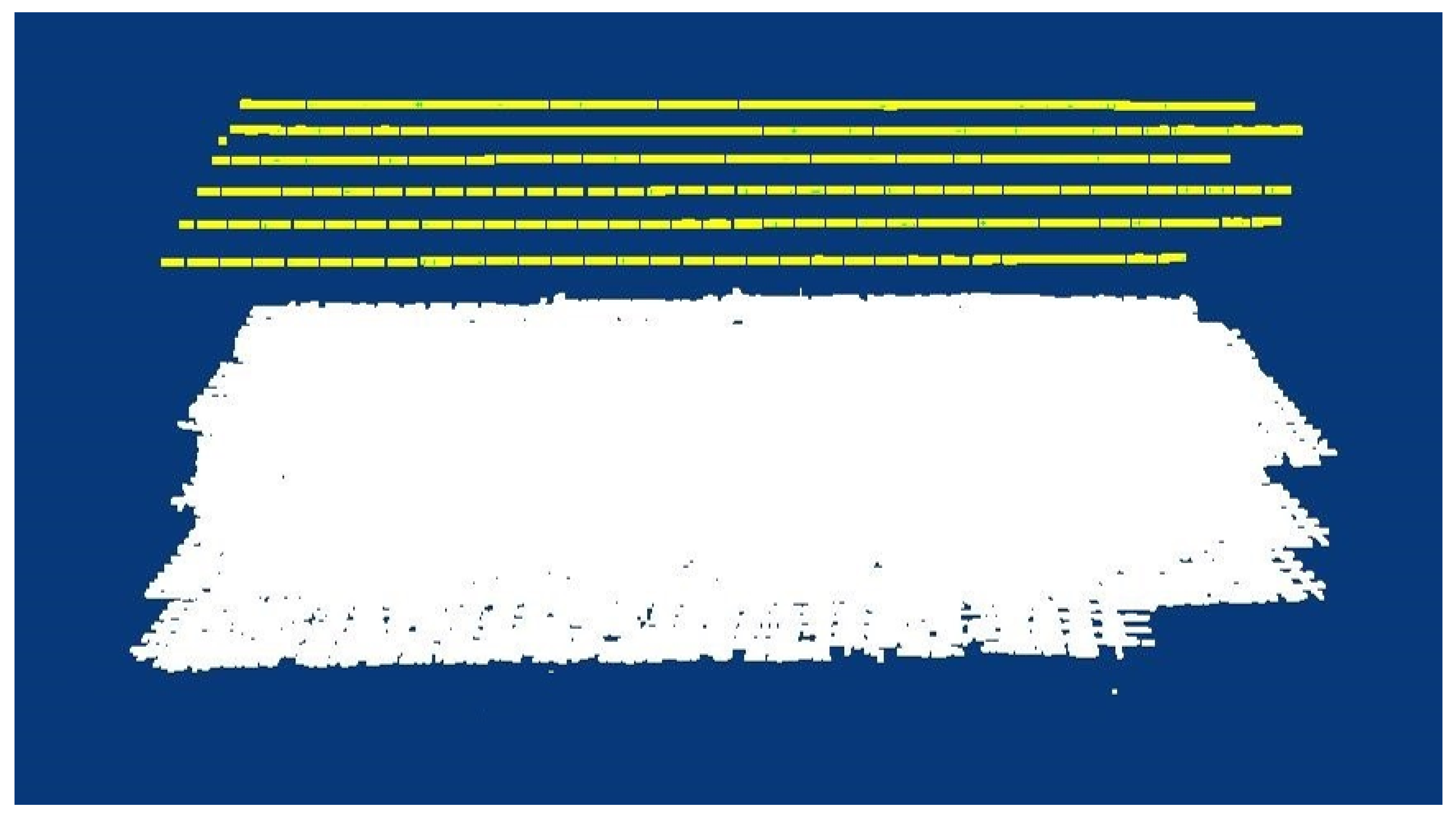
After BA processing, the sparse point cloud of the corresponding area is constructed. The ground point cloud and the corresponding camera projection center are shown in Figure 9. The yellow dashed lines illustrates the position of camera projection centers, and the white form is the ground point cloud.

As presented in Table 1, significant systematic errors were generated when without GCP support, particularly in the Z-axis. From Figure 9, the proposed method can produce a robust sparse, dense cloud.

5.3. The Proposed Method with GCP Support, but Not Considering Camera Intrinsic Parameters

The second experiment was carried out with the same set of images. Four ground control points contributed to the BA process, and the same checkpoints were used to evaluate the adjustment accuracy. A total of 3,091,007 pairwise point correspondences were extracted from matching. The statistical differences and RMSE are shown in

Table 3. Statistical Values for CHKS after the Second Experiment (Unit: meter).

ID of CHK	X-Axis	Y-Axis	Z-Axis
CHK 1	---	---	---
CHK 2	---	---	---
CHK 3	---	---	---
CHK 4	---	---	---
CHK 5	0.4117	1.0145	−1.6682
CHK 6	0.0062	0.0014	0.0068
CHK 7	---	---	---
CHK 8	---	---	---
CHK 9	−0.0573	0.0133	0.1149
CHK 10	−1.0118	−0.4301	0.0030
CHK 11	−0.0322	−0.0154	−0.0750
CHK 12	---	---	---
CHK 13	−0.0009	0.0054	−0.0014
RMSE	0.3035	0.3057	0.4642

.

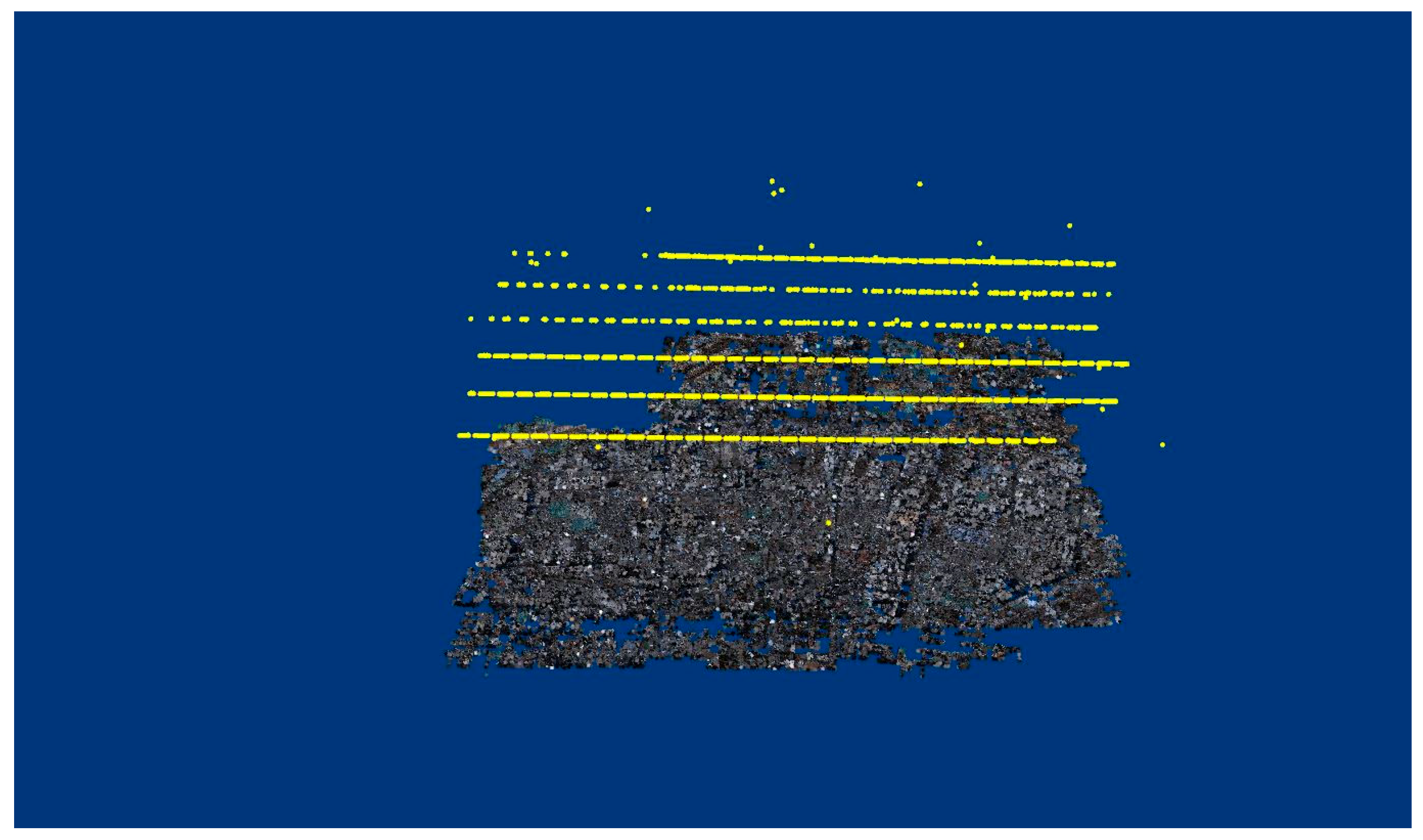
After BA adjustment with GCPs, the pairwise point correspondences were used to construct the sparse ground point cloud, as presented in Figure 10.

Since the intrinsic camera parameters were not adopted in the BA process, not all distortion sources were fully considered, and some images did not meet the consistency constraint. Therefore, image leaks occurred in the BA processing during the adjustment process; only 4567 images passed through the BA process. Since image leaks transpired in the BA process, some CHKs had no statistical residuals (see Table 3), and the sparse point cloud in Figure 10 lacks completeness and robustness.

5.4. The Proposed Method with GCP Support and Considering Camera Intrinsic Parameters

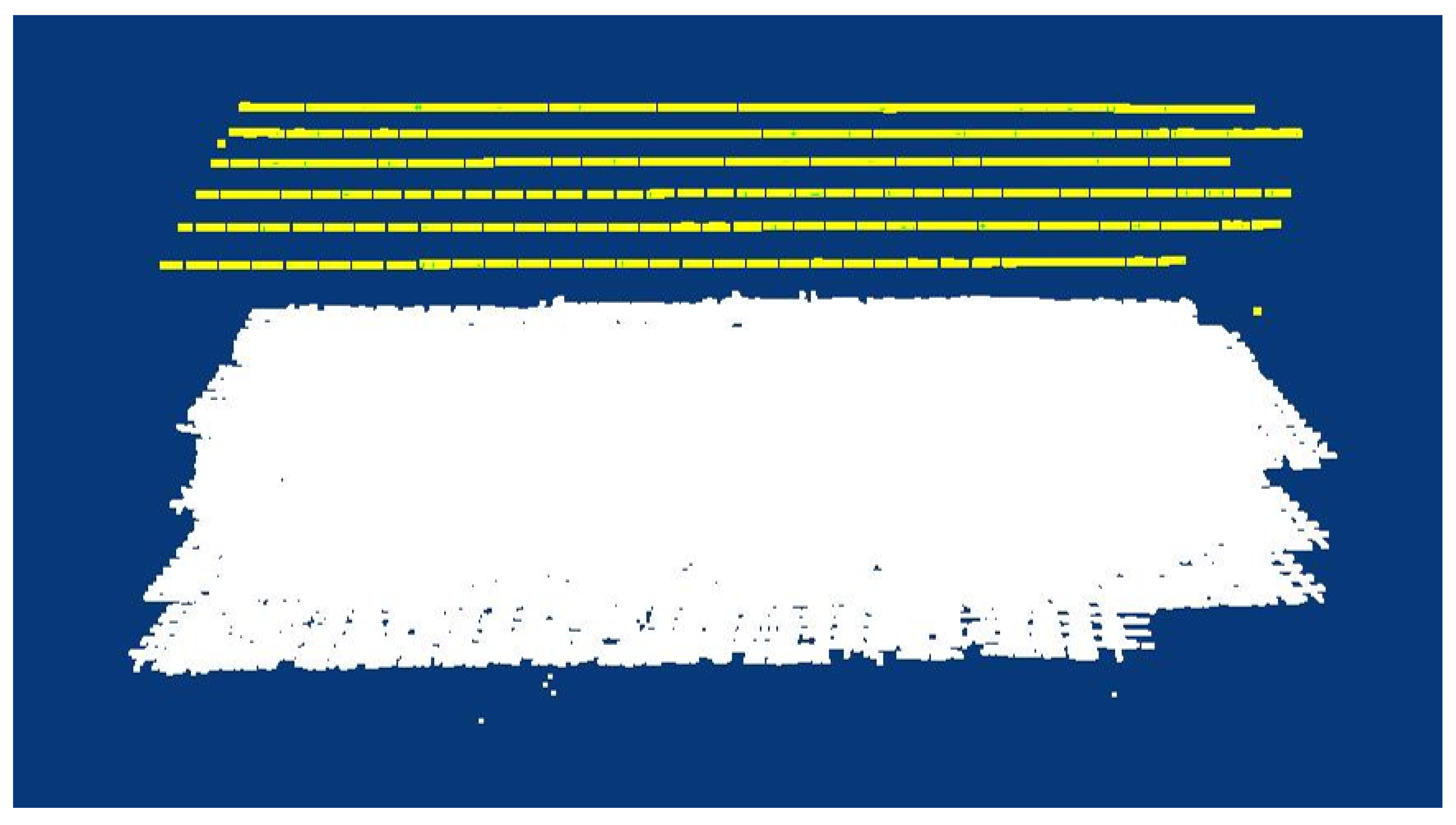
In the third experiment, a total of 6,884,305 pairwise point correspondences were extracted from matching. The residuals between the 3D observation and calculation values are summarized in

Table 4. Statistical Values for CHKS after the Third Experiment.

ID of CHK	X-Axis	Y-Axis	Z-Axis
CHK 1	−0.0081	−0.0001	0.0037
CHK 2	0.0035	0.0034	0.0028
CHK 3	−0.0089	−0.0529	−0.0722
CHK 4	0.0401	−0.0213	−0.0754
CHK 5	0.0571	−0.0411	0.0472
CHK 6	−0.0011	−0.0040	0.0107
CHK 7	−0.0364	−0.0023	−0.0755
CHK 8	−0.0157	−0.0030	−0.0250
CHK 9	−0.1061	0.0232	0.2133
CHK 10	−0.0450	0.0122	0.0258
CHK 11	−0.0034	0.0162	0.0015
CHK 12	0.0076	−0.0027	−0.0047
CHK 13	0.0005	−0.0035	−0.0001
RMSE	0.0392	0.0214	0.0711

. The sparse point cloud is shown in Figure 11. The intrinsic parameters before and after calibration are presented in

Table 5. The intrinsic parameters before and after calibration.

Parameter	Before Calibration	After Calibration
Principal Point x0 (pixel)	2432.0	2423.1399460647876
Principal Point y0 (pixel)	1616.0	1603.9860816155979
Calibration parameter 1	0	−0.14123671990384698
Calibration parameter 2	0	−27.234841758167391
Calibration parameter 3	0	3807.0519745535798
Calibration parameter 4	0	−0.00018113363239831057
Calibration parameter 5	0	−0.00069940821735464372

.

Table 3 show that the RMSE values for the 13 CHKs were below one pixel in the X and Y directions and below two pixels in the Z direction, equivalent to the precision obtained by the professional LightSpeed software [12,13,14,15]. The sparse point cloud shown in Figure 11 is much more complete and robust.

5.5. The Original OpenMVG SFM Pipeline with GCP Support

The fourth experiment was carried out using the original OpenMVG pipeline. All unknowns were considered, and the same group of GCPs and CHKs were used in the adjustment. A total of 6,797,129 pairwise point correspondences were extracted from matching. The statistical results are shown in

Table 6. Statistical Values for CHKS after the Fourth Experiment (Unit: meter).

ID of CHK	X-Axis	Y-Axis	Z-Axis
CHK 1	0.2285	−0.2146	0.3560
CHK 2	0.2223	−0.2655	−0.2265
CHK 3	0.2393	−0.2149	−0.2078
CHK 4	0.2362	−0.1163	0.2652
CHK 5	−0.1373	−0.2316	−0.1682
CHK 6	−0.0895	−0.1930	0.3068
CHK 7	0.2187	0.2328	0.1032
CHK 8	0.2167	0.2855	−0.1176
CHK 9	−0.2655	0.2211	0.2149
CHK 10	−0.2353	0.1838	0.2030
CHK 11	0.0215	0.2046	−0.1750
CHK 12	−0.2624	0.2395	0.1582
CHK 13	−0.2297	0.2441	−0.1014
RMSE	0.2998	0.3148	0.3017

. The sparse point cloud is displayed in Figure 12.

Table 6 show that the accuracy of the original OpenMVG SFM pipeline is far better than that of the first experiment and that no systematic errors remained in the result. However, the results were still not as good as those of the third experiment.

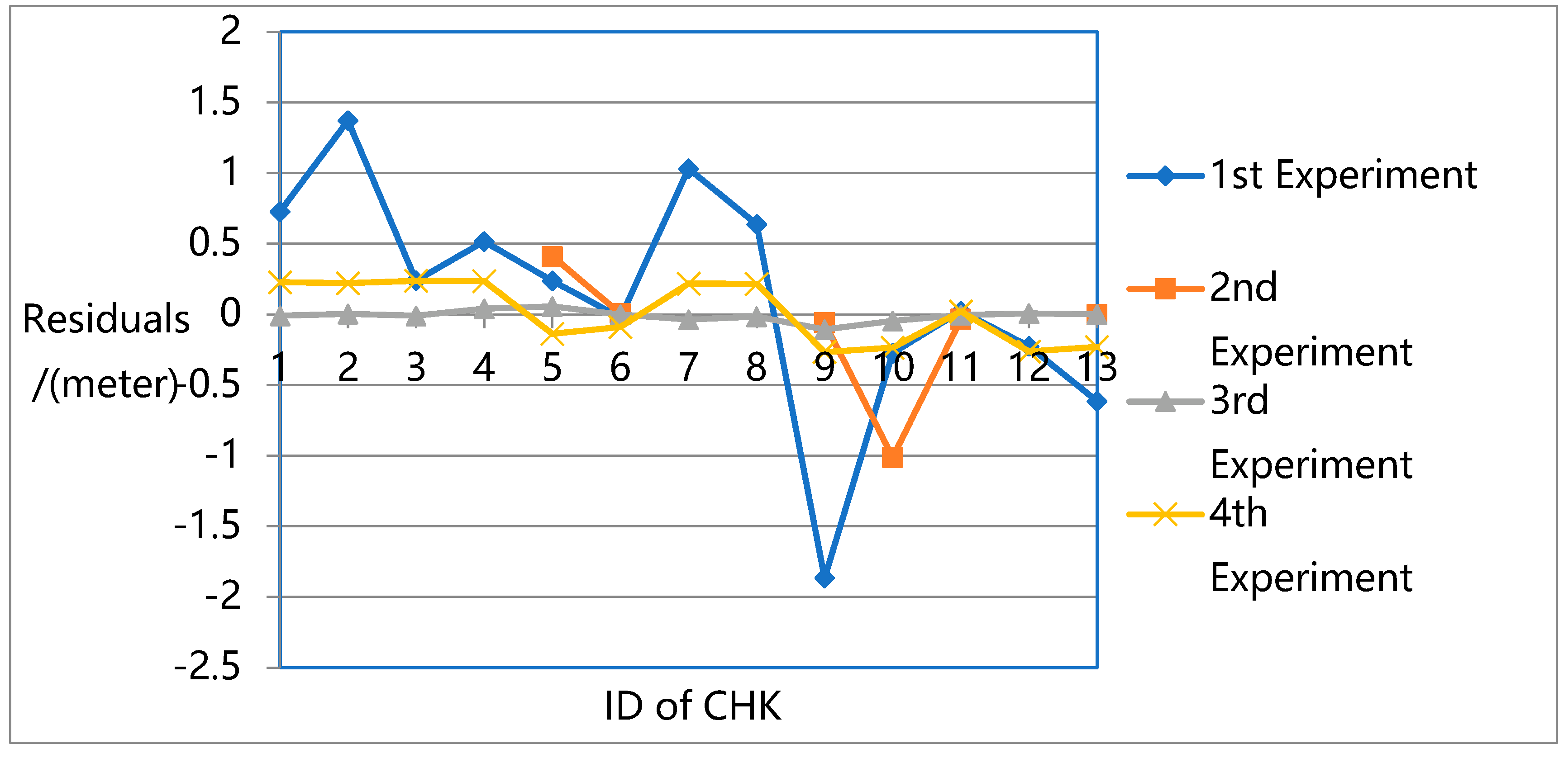
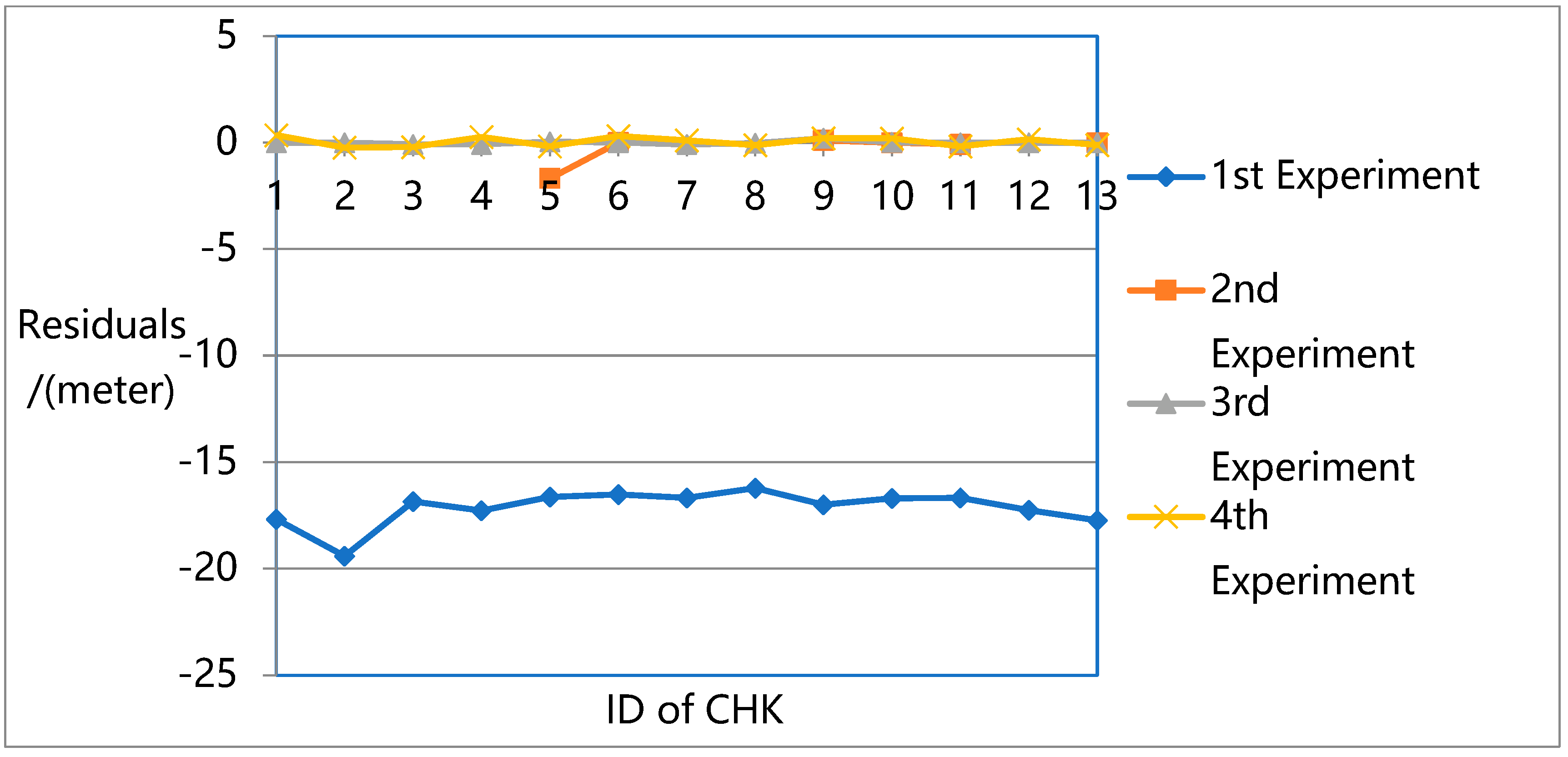
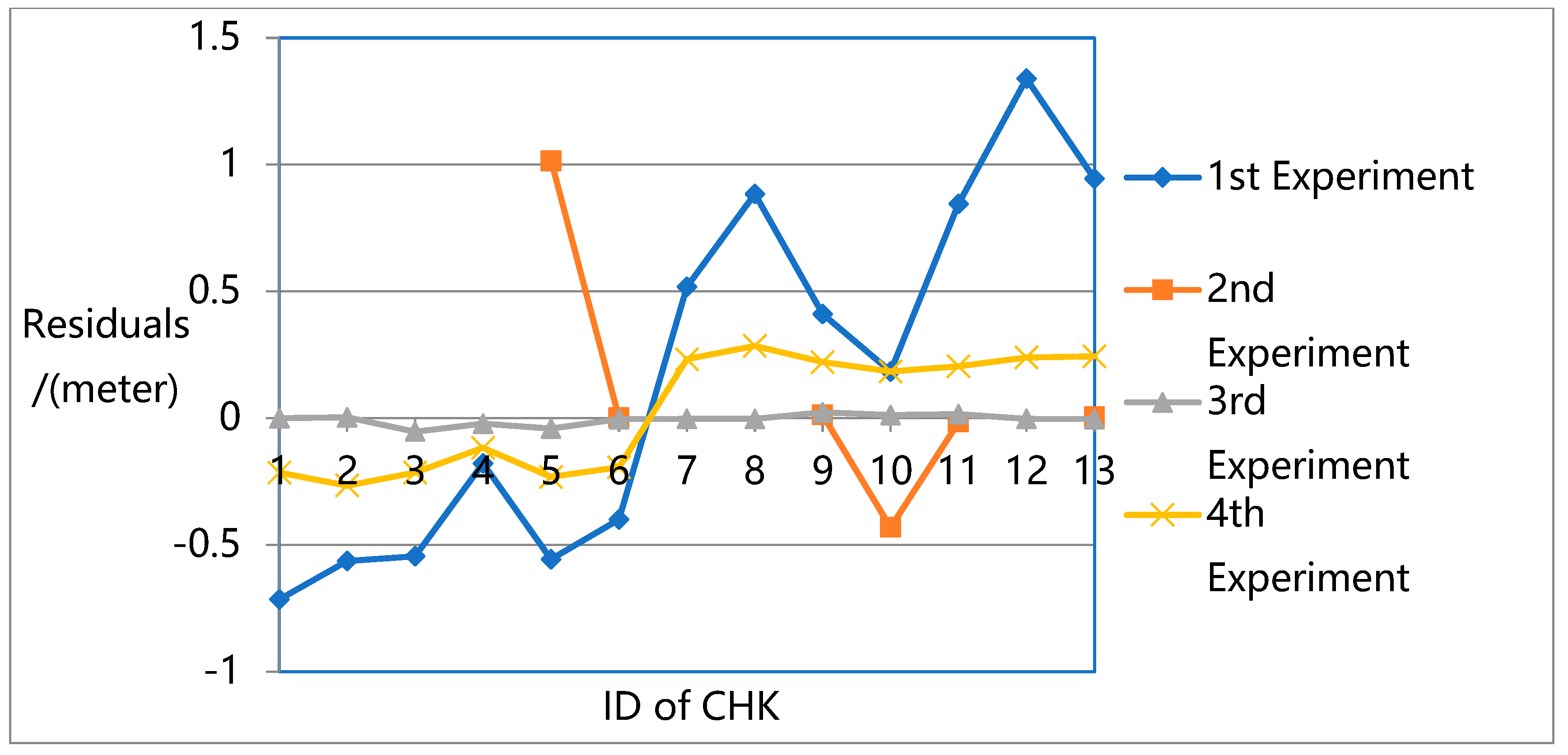
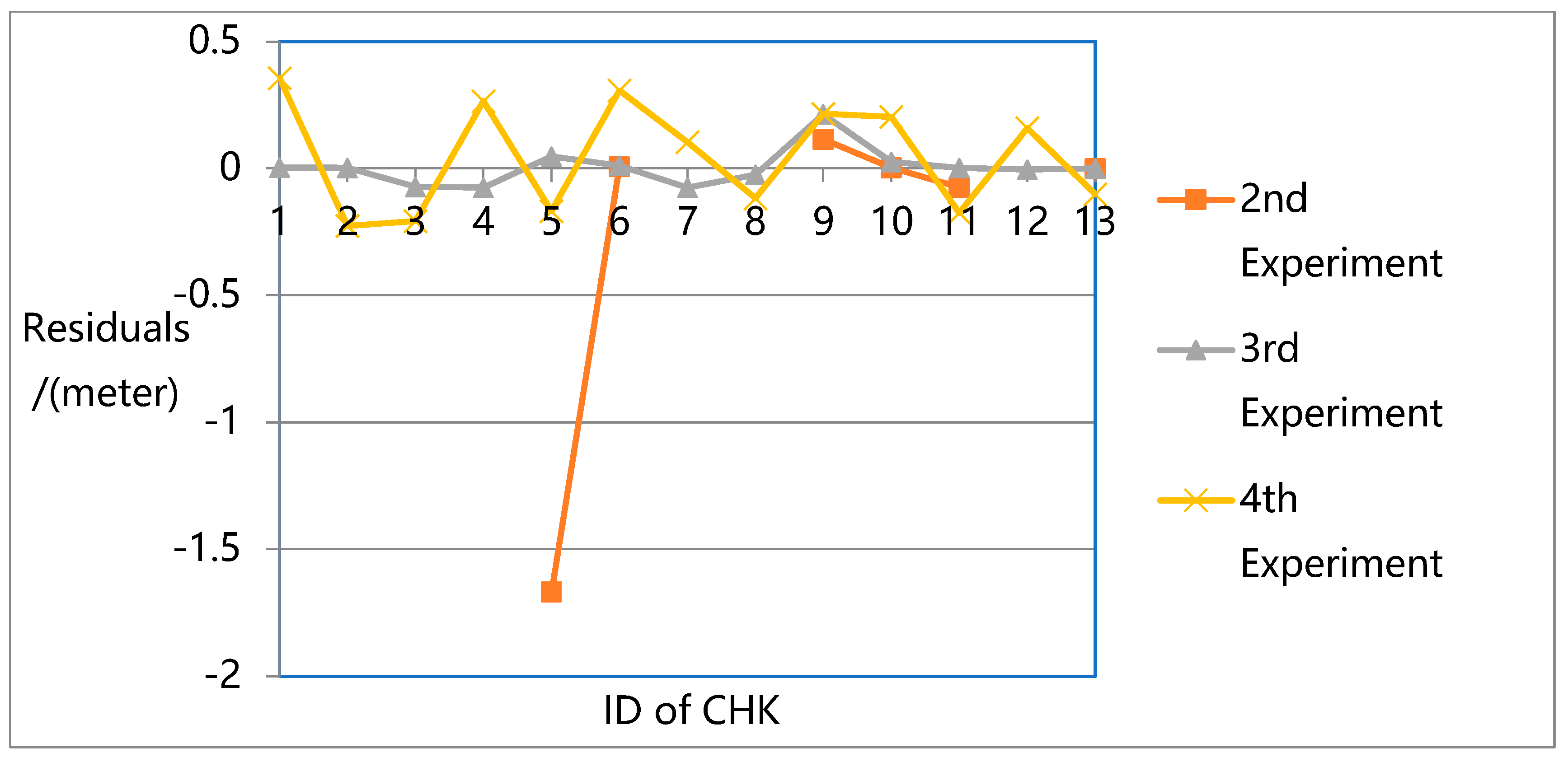
To better compare and analyze the different test results, the residuals from Table 2, Table 3, Table 4 and Table 6 were plotted. Figure 13 present the residuals at each CHK in the X-direction, Figure 14 show the residuals in the Y-direction, and Figure 15 provide the residuals in the Z-direction. Figure 16 present a more detailed comparison of residuals in the Z-direction.

The results show that the largest errors were found in the first experiment. While the first experiment deals with all the unknowns (e.g., rotation, translation, intrinsic parameters, and 3D ground point coordinates) in the overall flow and constructs a robust sparse point cloud, it does not eliminate the systematic errors in the pose data, especially in the Z direction. Due to the lack of ground truth guidance, even with GPS support, significant deviations could be found between the resulting 3D model and the ground truth.

For the second experiment, significant image leaks occurred due to the lack of intrinsic parameters in the adjustment. This means that for high oblique frame sweep images, intrinsic parameters are indispensable in adjustment. For normal vertical photogrammetric images, although the BA process is unable to attain the highest precision when intrinsic parameters are ignored, the robust bundle block can still be obtained.

In the third experiment, the highest precision is reached with a robust sparse point cloud. In the fourth experiment, with GPS and GCP data, the original OpenMVG pipeline can achieve high positioning accuracy in three directions with a robust sparse point cloud. However, its accuracy is not as high as that of the proposed quadrifocal tensor SFM photogrammetry method.

In the third and fourth experiments, while all the unknowns (e.g., rotation, translation, intrinsic parameters, and 3D ground point coordinates) are considered in the BA process, the proposed method achieves much higher accuracy. The proposed approach introduces the iterative photogrammetry idea into the original OpenMVG SFM pipeline following an aerial and satellite photogrammetry processing approach, focusing more on the imaging geometric principle and camera characteristics. Using iterative BA adjustment, the distortion sources are dealt with from a coarse to fine approach, enhancing the BA accuracy step by step.

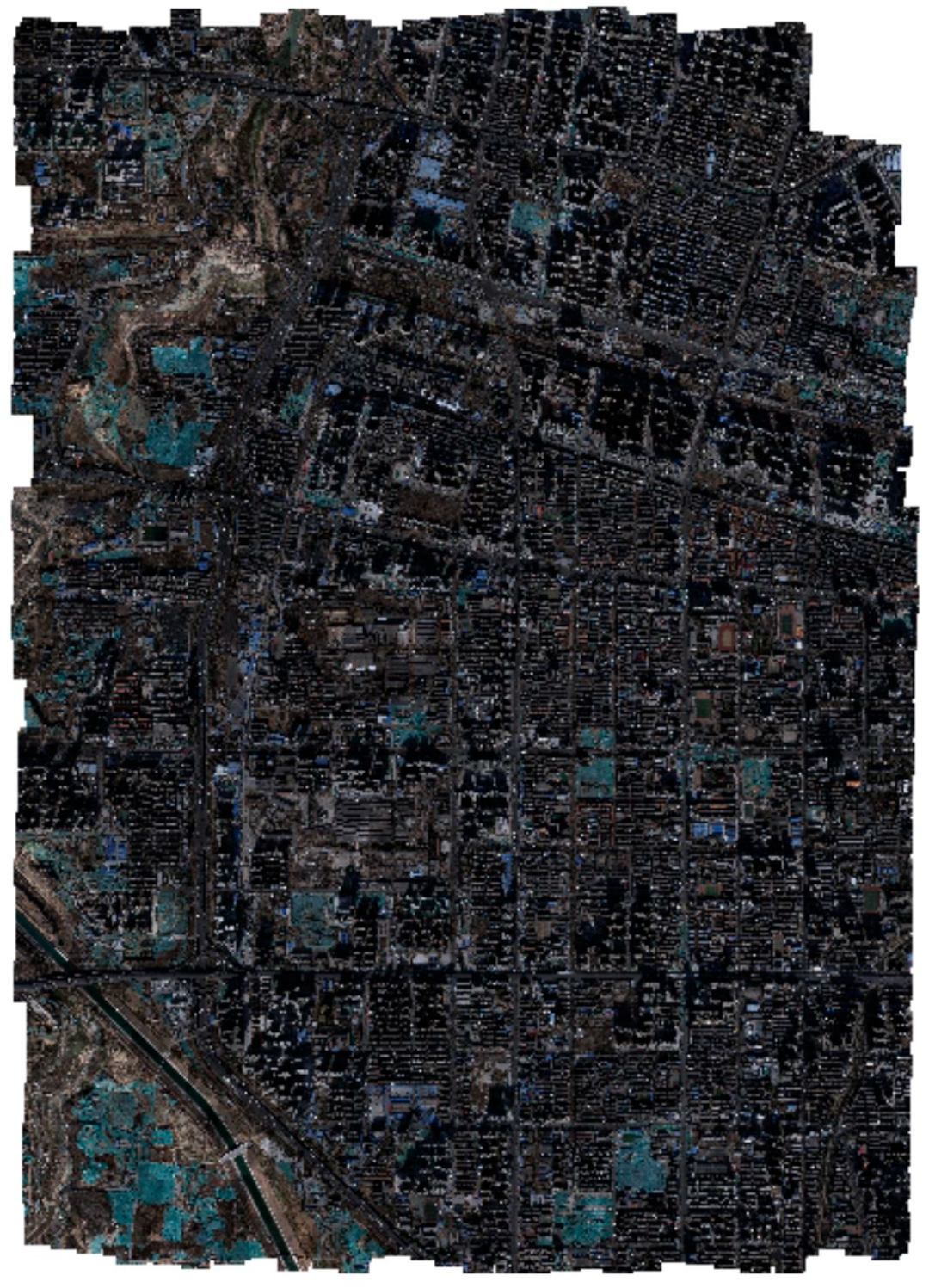
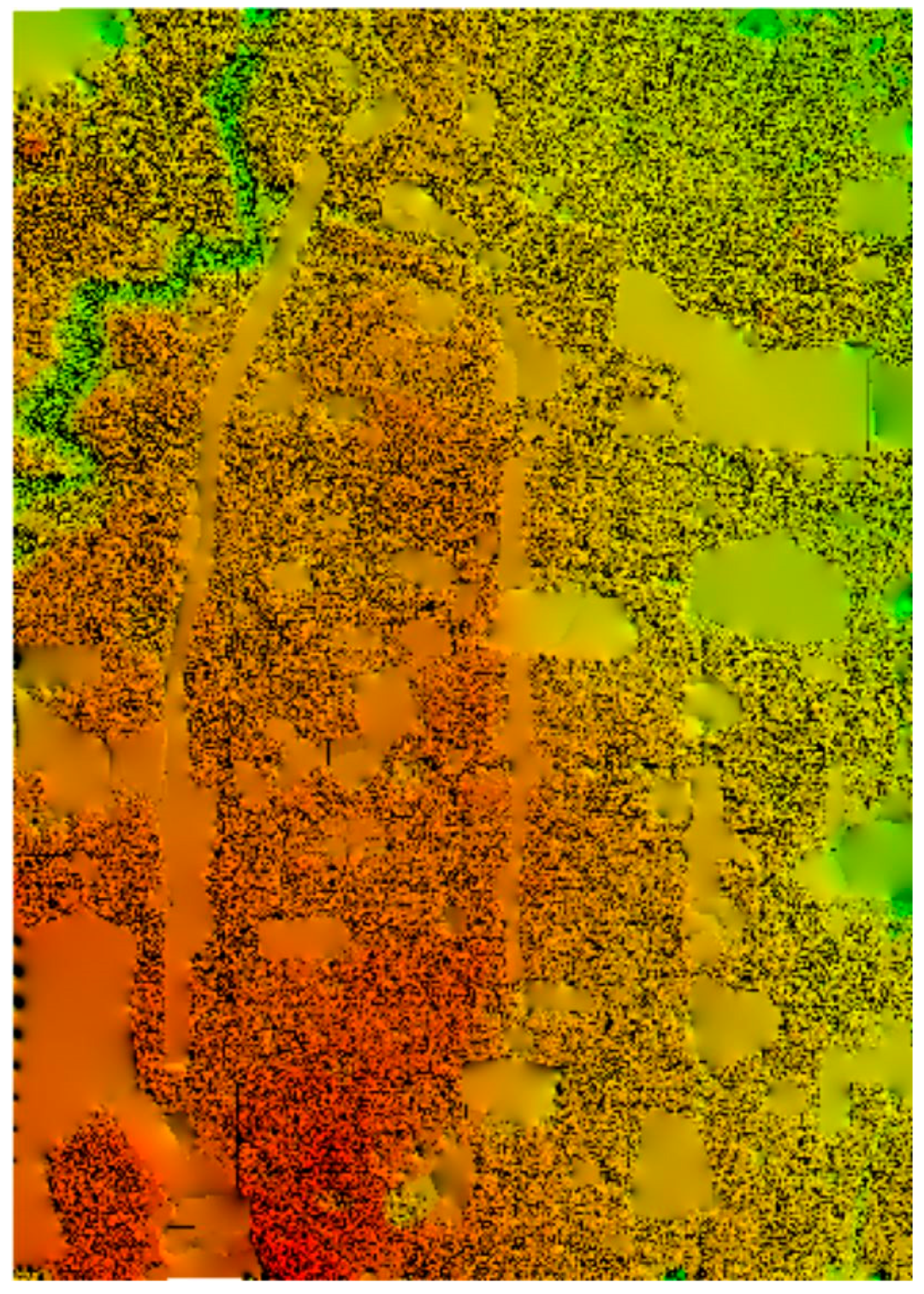
Figure 17 and Figure 18 show the digital orthophoto map (DOM) and digital elevation model (DEM) products after the BA positioning and calibration process in the third experiment. The ground resolution of the DOM and the DEM was set to 7 cm. Fifteen points were randomly selected from the DOM and DEM products. Measurements were then taken from the two products, and observation values were made in the field test. After comparing the values, the accuracy of the DOM was found to be from 1 to 3 pixels. The largest difference was 2.72 pixels, the smallest difference was 1.01 pixels, and the RMSE was 1.32 pixels. The DEM accuracy ranged from 2 to 5 pixels. The largest difference was 4.23 pixels, the smallest difference was 2.05 pixels, and the RMSE was 2.91 pixels.

LightSpeed software was then used for the given dataset, implementing the entire photogrammetry procedure and generating the DOM and DEM products. The photogrammetry results and the DOM and DEM products obtained using the two methods were compared and evaluated. The BA results and the DOM and DEM products obtained by the two approaches were at the same accuracy level, which suggests that our proposed method reaches the precision level of professional photogrammetry software.

6. Conclusions

Sweeping along the flight’s vertical direction for imaging, the frame sweep camera is characterized by a large field of view, a wide observation range, and a multi-angle imaging mode. While these characteristics can be useful for 3D reconstruction, they also increase the difficulty of image positioning. For large tilt oblique photogrammetry, the image positioning and calibration process becomes much more complex. Additionally, with the increasing integration between photogrammetry and SFM, more attempts have been made to combine these approaches to realize the positioning, calibration, and 3D reconstruction of large amounts of ordered or disordered images. After an extensive literature review and research, the OpenMVG pipeline was found to be most suitable for VisionMap A3 positioning and calibration.

Using the OpenMVG pipeline, a quadrifocal tensor-based positioning and calibration method was developed for high oblique frame sweep aerial cameras according to the imaging characteristics of VisionMap A3. We comprehensively analyzed the entire processing flow, from feature extraction and image matching, relative rotation and translation estimation, global rotation and translation estimation, and the quadrifocal tensor model construction to the BA process and calibration. Focusing on the imaging character of the VisionMap A3 camera, the quadrifocal tensor was put forward as the basis for BA adjustment. For the BA process and calibration, a coarse to fine three-stage BA processing modification was introduced in the OpenMVG pipeline following photogrammetric processing. Based on the experimental results, our main conclusions are as follows:

First, the SFM photogrammetric approach is suitable for large tilt oblique photogrammetry. When considering the rotation, translation, 3D ground coordinates, and the camera’s intrinsic parameters, the SFM pipeline, as OpenMVG, can generate a robust sparse point cloud.

Second, GPS data can only provide an initial value for the BA process. We found significant deviations between the processed bundle block and the ground control points. The results suggest that ground truth is still indispensable in positioning and calibration.

Third, the intrinsic parameters cannot be ignored in the BA process. The lack of intrinsic parameters resulted in image leaks in the bundle block and the sparse point cloud. The results indicate that the intrinsic parameters play an important role in dealing with inner and outer positioning errors.

Fourth, the coarse to fine processing approach in classical photogrammetry is still advisable in SFM photogrammetry. Processing the rotation (R) and translation (T) parameters eliminates most gross positioning errors while processing the intrinsic parameters propels the positioning precision to a higher level.

The experimental results on multiple overlapping routes of VisionMap A3 edge images suggest that our proposed method could achieve a robust bundle block and sparse point cloud and generate accurate DOM and DEM products. However, for the single route, the proposed method generated a bundle block with only contours, and the inner images were mostly considered outliers and excluded from the calculations. Subsequent studies are required to explore how to retain more images and effectively exclude outliers.