Calibration of MIMO Radar Transmitting and Receiving Array Using Scene Object Measurement

Abstract

The paper describes two simple methods allowing phase offsets to be aligned between radiators of transmitting and receiving antenna arrays in a collocated MIMO (Multiple Input Multiple Output) radar. One method uses normalization with averaging, while the second applies SVD (Singular Value Decomposition) of a measurement matrix. To calibrate phase offsets, the measurement of a calibration target at a known angular position must be done. The paper shows numerical comparison to already known method based on normalization by a single element of MIMO measurement matrix and experimental results obtained through the application of the proposed methods to measurement data.

1. Introduction

Recent scientific publications have shown the increasing interest of radar specialists in collocated MIMO (multiple input multiple output) radar [1]. Most papers contain results of simulation experiments, but the availability of SDR (software defined radio) platforms and increasing computational capacities of processors, including CPU, GPU, and FPGA, have created opportunities for the implementation of experimental systems [2,3]. In the case of MIMO with TDMA (time division multiplexing access) [4,5], the mass production of custom systems is expected, mainly serving as automotive sensors.

As for any antenna array, for MIMO radar the matter of phase calibration is crucial. Even when components are intended to be identical, they can differ due to manufacturing accuracy. Moreover, in CDMA (code division multiple access) MIMO, where each channel has a separate transmitter or receiver, the coherency between channels depends on the phase alignment of the carrier in modulators or demodulators. Cheaper platforms, which do not share the LO (local oscillator) signal, often start with the random initial phase of carrier synthesizers in otherwise coherent channels, which makes online calibration necessary for every run. Even in the higher-class platforms, thermal drifts can disturb phase offsets [6] and derate the accuracy of beamforming.

One solution to the problem is to implement an internal network of calibration connections; including couplers; switches; and, most inconveniently, additional receive and transmit channels [7]. This, of course, generates costs and increases system complexity and size. Unfortunately, the network does not allow one to compensate offsets in array radiators.

The use of an external calibrator, comprised of a transmitter for the calibration of the receive array and a receiver for the calibration of the transmit array, can mitigate the problem without expansion of radar hardware. Due to the fact that a scene scatterer intrinsically performs reception and retransmission, it can be used as a calibrator when its position is known and its echo can be discerned from other returns. In a standard phased array radar, it is only possible to calibrate the receive array in such a way, since the waveforms transmitted from different radiators sum up coherently, producing one waveform with spatially varied amplitude. However, in the case of a MIMO system, transmit phases can also be extracted after signal reception. Due to the orthogonality of transmitted signals, the phase shift for each combination of transmit–receive paths can be extracted. Moreover, the information about phase shifts is excessive, and some averaging can be applied to increase accuracy. This paper describes two simple procedures allowing for the calculation of useful information from measurement data and the separate correction vectors for receive and transmit arrays to be obtained. It is assumed that the coupling effects between antennas can be neglected, or their effects are already incorporated into calibration coefficients.

The proposed algorithms outrun simple normalization in two aspects. Firstly, due to applied averaging, they exclude noise or other unwanted components. Secondly, the primary output consists of separate offsets for the transmit and receive array, which can be very useful when MIMO radar is going to be switched to a conventional phased array on transmit, for example for track confirmation. To form the transmit beam, a calibration vector for the transmit array is needed before the observation. The idea has been preliminarily presented in [8] and this work is an expansion, also showing results of its application to real measurement data and more detailed performance analyses.

There have been already several papers on MIMO radar calibration presented, but they mostly do not exactly cover the same topic as this. The papers either show the basic calibration by normalization by reference target [9,10] that does not fully benefit from data excess available in MIMO; or they describe very sophisticated methods, including antenna coupling or multitarget calibration on an unknown scene. These methods need the solution of constrained optimization, and they often cannot be implemented in real time. This paper fits the gap between those two classes of calibration approaches, which is the most important new quality. The proposed methods offer both maximal simplicity together with good performance allowed by utilization of MIMO data structure. A brief overview of available works is presented below.

In [11], the idea of post calibration of MIMO transmit array was presented, which is a crucial benefit in this type of radar. The calibration procedure details however have not been revealed. The method used was applied only to transmit array, so benefit from received data excess was not utilized. Another paper describes a FMCW (frequency modulated continuous waveform) MIMO radar [12]. The calibration method is based on a selected target of a known angular position. Its uncalibrated echo response was extracted and then compared with an ideal response. The procedure was done on a vectorized MIMO response vector, and it did not exploit a MIMO data structure. Moreover, the paper does not take into account the situation in which there are several targets at the same angle during calibration, which is a likely scenario.

On the other hand, a more complex algorithm can be derived, that use multiple targets, either sparse [13] or evenly distributed [14]. The main difficulty is that they must solve a quite complex optimization problem that has no closed from solution. It is a completely different class of problem approach, which will not be discussed in this paper.

The method equivalent to normalization and averaging from this paper was described in very recent publication [15], which shows relevance and novelty of the topic. The results are shown for simultaneous calibration on multiple targets. The results are presented in a different way but they generally support the idea that normalization with averaging constitute a major step in simple and fast calibration of MIMO arrays. However, the reference does not mention the method based on SVD, which has superior performance for low signal to noise ratios.

The structure of the paper is as follows. In Section 2, the signal and error model is introduced. Section 3 describes proposed methods of calibration. Section 4 shows results of performance simulation for separate calibration of transmit and receive arrays, while Section 5 presents results for a whole MIMO channel matrix. Section 6 contains a description and results of field measurements. Finally, Section 7 is the summary of the paper.

2. Signal Model

The radar works in CDMA MIMO mode, simultaneously transmitting a set $K$ of orthogonal, narrowband RF signals on a chosen carrier frequency. Each waveform is transmitted with one of the radiators, together constituting a collocated transmit array. The radiated signals are based on complex digital waveforms $\mathit{x}{\left(n\right)}_{K\times 1}$, which were synthesized with DACs (digital to analog converters) and upconverted using an IQ modulator. An integer index $n$ describes the sample number.

The processing is applied to a set of received complex baseband waveforms $\mathit{y}{\left(n\right)}_{L\times 1}$, captured with $L$ receive antennas grouped in an array. Waveforms were downconverted with quadrature demodulators and sampled using ADCs (Analog to Digital Converters).

If the observed echo contains the response of only one target at angle ${\mathsf{\Phi }}_0$, each element of $\mathit{y}\left(n\right)$ is a superposition of delayed, modulated, and scaled copies of transmitted waveforms and additive, spatially uncorrelated noise.

After the up- and downconversion of a narrowband signal, the signal delay differences between array elements and the target position are reduced to phase shifts that can be incorporated into phases of the transmit and receive array steering vectors $\mathit{a}\left(\mathsf{\Phi }\right)$ and $\mathit{b}\left(\mathsf{\Phi }\right)$:

$$\mathit{a}\left(\mathsf{\Phi }\right)={\left[{\mathrm{e}}^{-\mathrm{j}{\omega }_c{\tau }_{Tx1}\left(\mathsf{\Phi }\right)},\cdots ,{\mathrm{e}}^{-\mathrm{j}{\omega }_c{\tau }_{TxK}\left(\mathsf{\Phi }\right)}\right]}^{\mathit{T}},$$

(1)

$$\mathit{b}\left(\mathsf{\Phi }\right)={\left[{\mathrm{e}}^{-\mathrm{j}{\omega }_c{\tau }_{Rx1}\left(\mathsf{\Phi }\right)},\cdots ,{\mathrm{e}}^{-\mathrm{j}{\omega }_c{\tau }_{RxK}\left(\mathsf{\Phi }\right)}\right]}^{\mathit{T}}.$$

(2)

where ${\omega }_c$ is the carrier pulsation and $\tau \left(\mathsf{\Phi }\right)$ are relative delays between signals transmitted or received by subsequent array elements. The expressions above can describe the array behavior for any array geometry, including 2D arrays, if $\mathsf{\Phi }$ is replaced with a vector of azimuth and elevation.

The signal model for MIMO radar can be expressed as

$$\mathit{y}\left(n\right)=\alpha {\mathrm{e}}^{-\mathrm{j}{\mathsf{\vartheta }}_{D}n}\mathit{A}\left({\mathsf{\Phi }}_0\right)\mathit{x}\left(n-d\right)+\mathit{w}\left(n\right),$$

(3)

where $\alpha$ is the amplitude scaling factor depending on system gains, target reflectivity and range, ${\mathsf{\vartheta }}_D$ is Doppler pulsation normalized by the sampling frequency, $d$ is the delay proportional to target range expressed in the fractional multiple of the sample index, and $\mathit{w}{\left(n\right)}_{L\times 1}$ is additive complex Gaussian noise.

The channel matrix $\mathit{A}(\mathsf{\Phi }$) (Figure 1) for target direction $\mathsf{\Phi }$ is a product of steering vectors:

$$\mathit{A}\left(\mathsf{\Phi }\right)=\mathit{b}\left(\mathsf{\Phi }\right){\mathit{a}}^T\left(\mathsf{\Phi }\right).$$

(4)

The most basic processing flow for a collocated CDMA MIMO radar involves calculation of a set of crosscorrelation functions for each transmit–receive pair. If moving targets are considered, crossambiguity functions are calculated instead. The beamforming can be done on waveforms before the crossambiguity calculation, on crossambiguity functions or on particular range-velocity cells containing detected targets. Each solution is a compromise between computational complexity and achievable detection performance. In this case, it is assumed that for calibration purposes SNR (signal to noise ratio) is not an issue, and all operations can be done on an extracted cell containing target echo. In the rest of this work, without loss of generality, it will be assumed that the delay and the modulation of the cell are already compensated.

In such a case, the correlator output ${\mathit{Z}}_{K\times L}$ representing a single cell for all transmit–receive pairs is presented in a form of a matrix:

$$\mathit{Z}\left({\mathsf{\Phi }}_0\right)=\frac{1}{N}{\displaystyle \sum }_N\mathit{y}\left(n\right){\mathit{x}}^H\left(n\right)=\alpha \mathit{A}\left({\mathsf{\Phi }}_0\right){\mathit{R}}_{\mathit{x}\mathit{x}}+\mathit{V}$$

(5)

where ${\mathit{R}}_{\mathit{x}\mathit{x} K\times K}$ is the spatial correlation matrix of transmitted signals. ${\mathit{V}}_{K\times L}$ is the spatial cross-correlation matrix between reference signals and noise, and it describes noise that was suppressed during the integration (matched filtering) process.

Matrix ${\mathit{R}}_{\mathit{x}\mathit{x}}$ is a spatial correlation matrix, showing how similar signals transmitted with different antennas are expressed according to the following formula:

$${\mathit{R}}_{\mathit{x}\mathit{x}}=\mathrm{E}\left\{\mathit{x}\left(n\right){\mathit{x}}^H\left(n\right)\right\}\approx \frac{1}{N}{\displaystyle \sum }_N\mathit{x}\left(n\right){\mathit{x}}^H\left(n\right),$$

(6)

where the first version is theoretical, and the latter is a sample estimate obtained with $N$ samples. If the transmitted signals are orthogonal, as should be the case for MIMO, the matrix has only diagonal elements. The estimate, however, may have non zero entries if the waveforms are not truly orthogonal. Matrix $\mathit{V}$ is expressed in a similar way:

$$\mathit{V}=\mathrm{E}\left\{\mathit{w}\left(n\right){\mathit{x}}^H\left(n\right)\right\}\approx \frac{1}{N}{\displaystyle \sum }_N\mathit{w}\left(n\right){\mathit{x}}^H\left(n\right).$$

(7)

The signal model above is widely used for the description of collocated MIMO radar [16,17,18].

The direction-finding in the most basic case, using conventional beamforming with equal noise powers in receive channels and no spurious directional signals, consists of finding the maximum of function:

$$\widehat{P}\left(\mathsf{\Phi }\right)={\left|{\mathit{h}}^H\left(\mathsf{\Phi }\right)\mathit{z}\right|}^2,$$

(8)

where $\mathit{z}$ is vectorized matrix $\mathit{Z}$, and h is a spatial filter that in its simplest form without normalization is a model of ideal response from direction $\mathsf{\Phi }$, also in vectorized form:

$$\mathit{h}=\mathrm{vec}\left\{\mathit{A}\left(\mathsf{\Phi }\right)\right\}.$$

(9)

The problem described in this paper addressed a situation when the measured signal was obtained from steering vectors perturbed with unknown relative phase shifts between channels (Figure 2) that, using the Hadamard product, can be expressed as complex vectors $\mathsf{\Delta }\mathit{a}$ and $\mathsf{\Delta }\mathit{b}$, so that

$$\tilde{\mathit{a}}\left(\mathsf{\Phi }\right)=\mathit{a}\left(\mathsf{\Phi }\right)\circ \mathsf{\Delta }\mathit{a},$$

(10)

$$\tilde{\mathit{b}}\left(\mathsf{\Phi }\right)=\mathit{b}\left(\mathsf{\Phi }\right)\circ \mathsf{\Delta }\mathit{b} .$$

(11)

As a result, we want to extract $\mathsf{\Delta }\mathit{a}$ and $\mathsf{\Delta }\mathit{b}$ from the perturbed measurement response

$$\tilde{\mathit{Z}}\left({\mathsf{\Phi }}_0\right)=\alpha \tilde{\mathit{A}}\left({\mathsf{\Phi }}_0\right){\mathit{R}}_{\mathit{x}\mathit{x}}+\mathit{V},$$

(12)

knowing proper theoretical vectors $\mathit{a}\left({\mathsf{\Phi }}_0\right)$ and $\mathit{b}\left({\mathsf{\Phi }}_0\right)$. Due to the orthogonality of the transmitted signals, ${\mathit{R}}_{\mathit{x}\mathit{x}}$ is assumed to be an identity matrix, and it can be omitted.

3. Proposed Methods

The first step of analysis is to find a basic way to extract $\mathsf{\Delta }\mathit{A}=\mathsf{\Delta }\mathit{b}\mathsf{\Delta }{\mathit{a}}^T$. It can be shown using properties of the Hadamard product [19] that

$$\tilde{\mathit{A}}=\mathit{b}{\mathit{a}}^T\circ \mathsf{\Delta }\mathit{b}\mathsf{\Delta }{\mathit{a}}^T=\left(\mathit{b}\circ \mathsf{\Delta }\mathit{b}\right)\left({\mathit{a}}^T\circ \mathsf{\Delta }{\mathit{a}}^T\right)=\mathit{A}\circ \mathsf{\Delta }\mathit{A}.$$

(13)

It is evident that to get an initial estimate of $\mathsf{\Delta }\mathit{A}$, the response $\tilde{\mathit{Z}}$ should be elementwise divided by $\mathit{A}\left({\mathsf{\Phi }}_0\right)$

$$\mathsf{\Delta }{\widehat{\mathit{A}}}_{i,j}=\frac{{\tilde{\mathit{Z}}}_{i,j}}{{\mathit{A}}_{i,j}\left({\mathsf{\Phi }}_0\right)}.$$

(14)

This provides calibration coefficients for the MIMO mode. This approach has two major flaws. Firstly, it is vulnerable to noise component $\mathit{V}$. The whole process depends strongly on the particular realization of a random variable. Secondly, it does not allow one to separate offsets of transmitting and receiving arrays, which is needed for phased array operation with physical beamforming on transmission.

There are at least two ways to extract $\mathsf{\Delta }\widehat{\mathit{a}}$ and $\mathsf{\Delta }\widehat{\mathit{b}}$ estimates, utilizing knowledge of the $\mathsf{\Delta }\widehat{\mathit{A}}$ structure. The first is based on normalization and averaging, while the second uses SVD decomposition.

A.

Normalization and averaging

In order to calculate the estimate $\mathsf{\Delta }\widehat{\mathit{a}}$, one can normalize $\mathsf{\Delta }\widehat{\mathit{A}}$ by elementwise division of each column by the first one (or any other set as the reference) as depicted in the Figure 3. In this paper, it is assumed that at each array channel the transmitted (or received) power are statistically equal and no tapering is applied.

$$\mathsf{\Delta }{\check{\mathit{A}}}_{i,j}=\frac{\mathsf{\Delta }{\widehat{\mathit{A}}}_{i,j}}{\mathsf{\Delta }{\widehat{\mathit{A}}}_{i,1}}$$

(15)

and then perform averaging in the vertical direction:

$$\mathsf{\Delta }{\widehat{\mathit{a}}}_j^{*}=\frac{1}{\mathrm{L}}{\displaystyle \sum }_l\mathsf{\Delta }{\check{\mathit{A}}}_{l,j}.$$

(16)

Similarly, vector $\mathsf{\Delta }\widehat{\mathit{b}}$ can be obtained by row normalization (Figure 4):

$$\mathsf{\Delta }{\check{\mathit{A}}}_{i,j}=\frac{\mathsf{\Delta }{\widehat{\mathit{A}}}_{i,j}}{\mathsf{\Delta }{\widehat{\mathit{A}}}_{1,j}}$$

(17)

and then averaging in the vertical direction:

$$\mathsf{\Delta }{\widehat{\mathit{b}}}_i=\frac{1}{\mathrm{K}}{\displaystyle \sum }_k\mathsf{\Delta }{\check{\mathit{A}}}_{i,k .}$$

(18)

Such vectors can be used to reevaluate matrix $\Delta \widehat{\mathit{A}}$ with a decreased noise influence.

• B. SVD decomposition

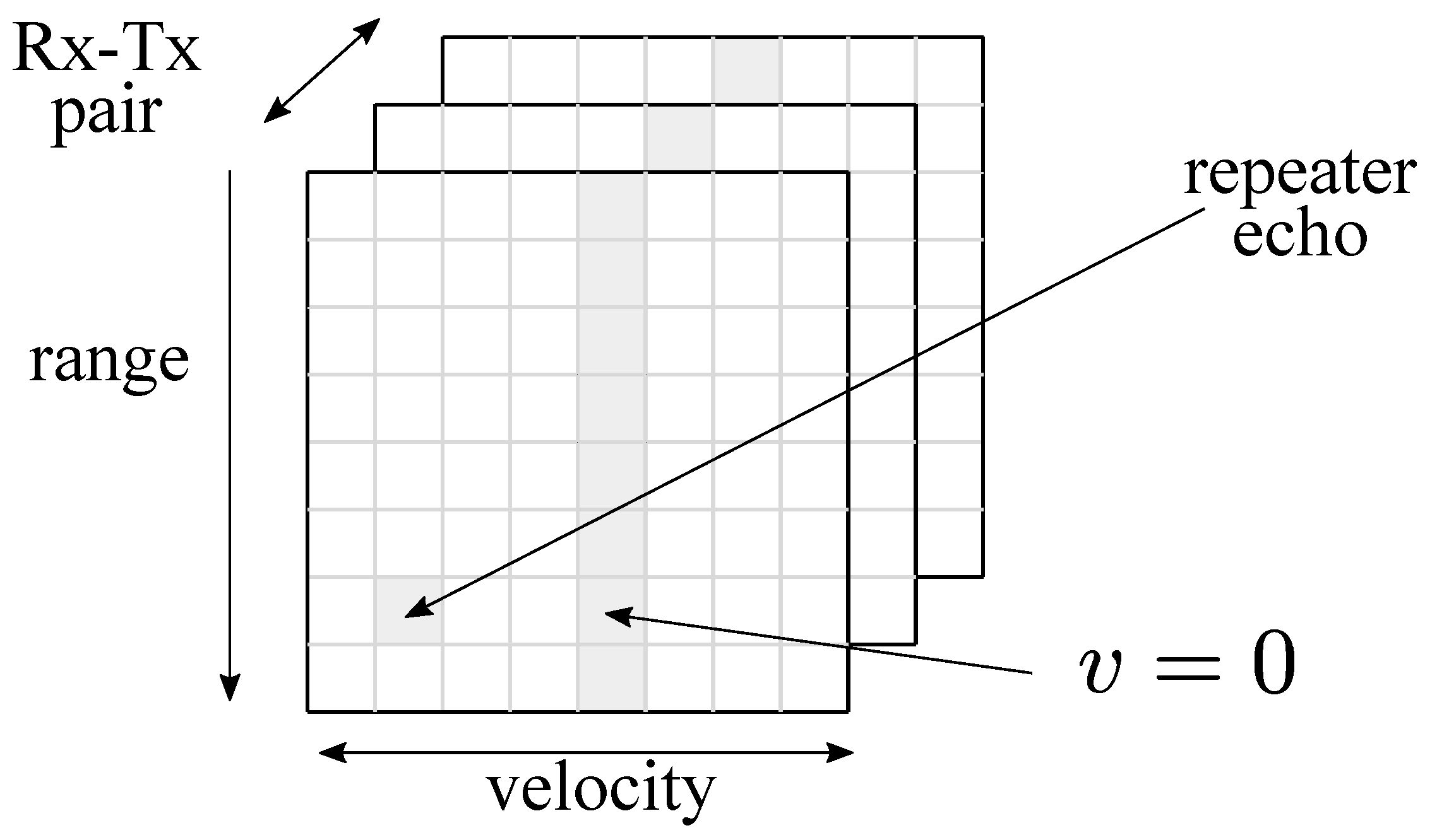
The other approach uses a known property of SVD decomposition [20]:

$$\mathsf{\Delta }\widehat{\mathit{A}}=\mathit{U}\mathrm{diag}\left\{{\mathsf{\sigma }}_i\right\}{\mathit{V}}^H={\displaystyle \sum }_i\mathsf{\Delta }{\widehat{\mathit{A}}}_i={\displaystyle \sum }_i{\mathsf{\sigma }}_i{\mathit{u}}_i\otimes {\mathit{v}}_i$$

(19)

according to which, if matrix $\mathsf{\Delta }\widehat{\mathit{A}}$ has a component that can be expressed as the outer product of two vectors, it would be assigned to a particular singular value, and those vectors will appear as columns of $\mathit{U}$ and $\mathit{V}$ matrices (Figure 5). If there is only one strong directional echo from the calibrator, taking into account (2), the signal fulfils this assumption, and the estimates will be

$$\mathsf{\Delta }{\widehat{\mathit{a}}}_{j,1}={\mathit{U}}_{j,1},$$

(20)

$$\mathsf{\Delta }{\widehat{\mathit{b}}}_{i,1}={\mathit{V}}_{i,1}^{*}$$

(21)

The noise components that do not follow the pattern are related to further singular values ${\sigma }_i$, that have random, small values. By zeroing those unwanted values, one can obtain a denoised estimate of $\mathsf{\Delta }\widehat{\mathit{A}}$. Vectors $\mathsf{\Delta }\widehat{\mathit{a}}$ and $\mathsf{\Delta }\widehat{\mathit{b}}$ can also be normalized by the first (or any other) component to get relative phase and amplitude offsets.

4. Numerical Evaluation of Steering Vector Offsets

Both methods were examined in simulations performed in the Matlab environment. Separate 10-element transmit and 20-element receive linear arrays were defined with a half-wavelength spacing between transmit radiators and two-wavelength spacing between receiving ones, thus forming a uniform virtual array called a Nyquist array [21]. The simulation was done according to (12) with calibration target in far-field, arbitrarily placed at angle ${\mathsf{\Phi }}_0=5°.$

The general statistical performance of both methods has been verified. A single realization of the experiment consisted of the generation of vectors $\mathsf{\Delta }\mathit{a}$ and $\mathsf{\Delta }\mathit{b}$, with uniformly distributed random phase shifts and unitary amplitudes. The vectors were then normalized by the first element to express relative phase shifts. In addition, the noise matrix $\mathit{V}$ was generated as a set of uncorrelated complex Gaussian samples with zero mean and variance related to the post-correlation signal power to noise ratio.

What is interesting is the phase difference between the base value of vector coefficients and its estimate. For a sufficiently high signal to noise power ratio (SNR), the phase error is small enough, and it does not wrap, so the calculation of standard deviation is reasonable.

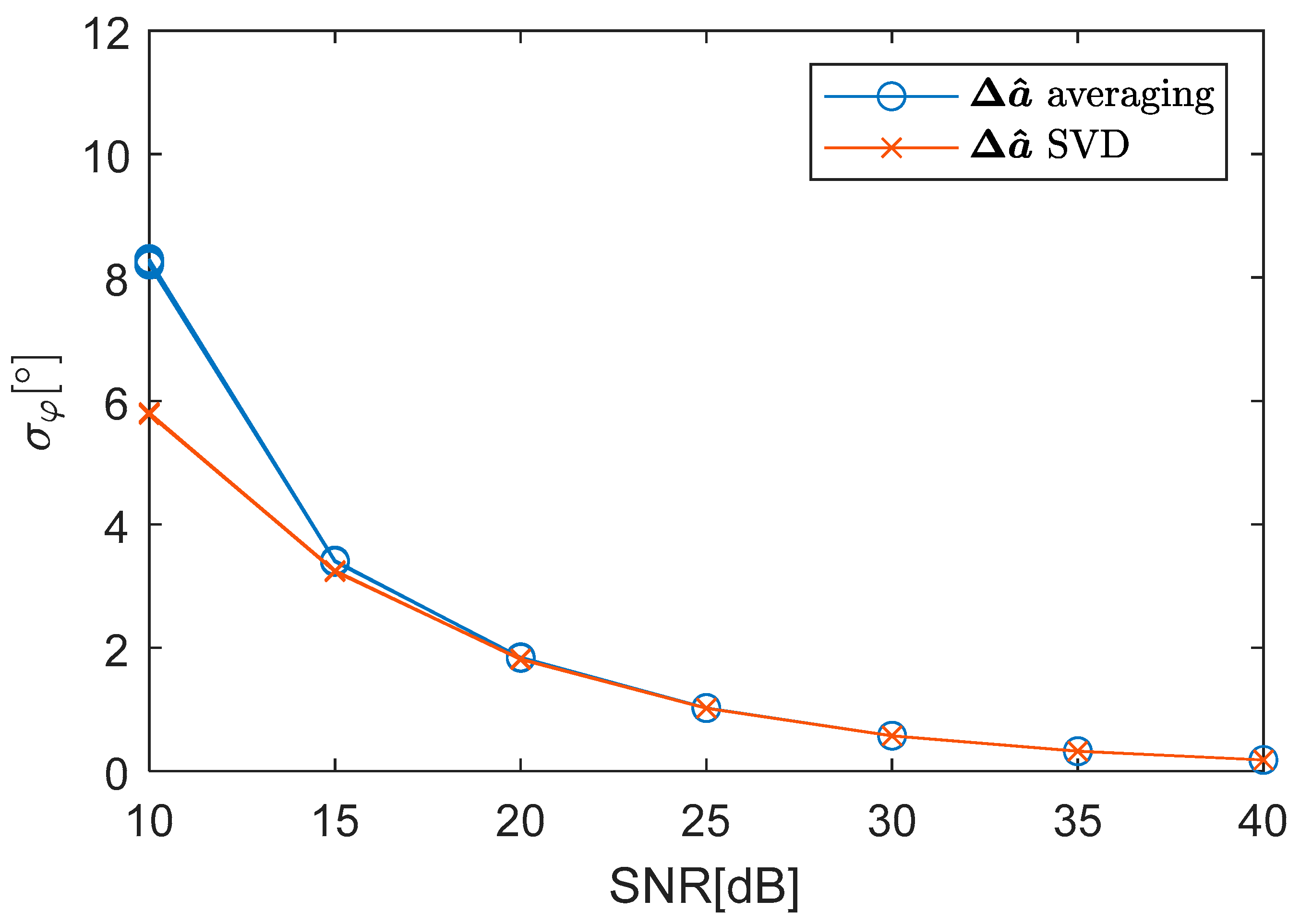
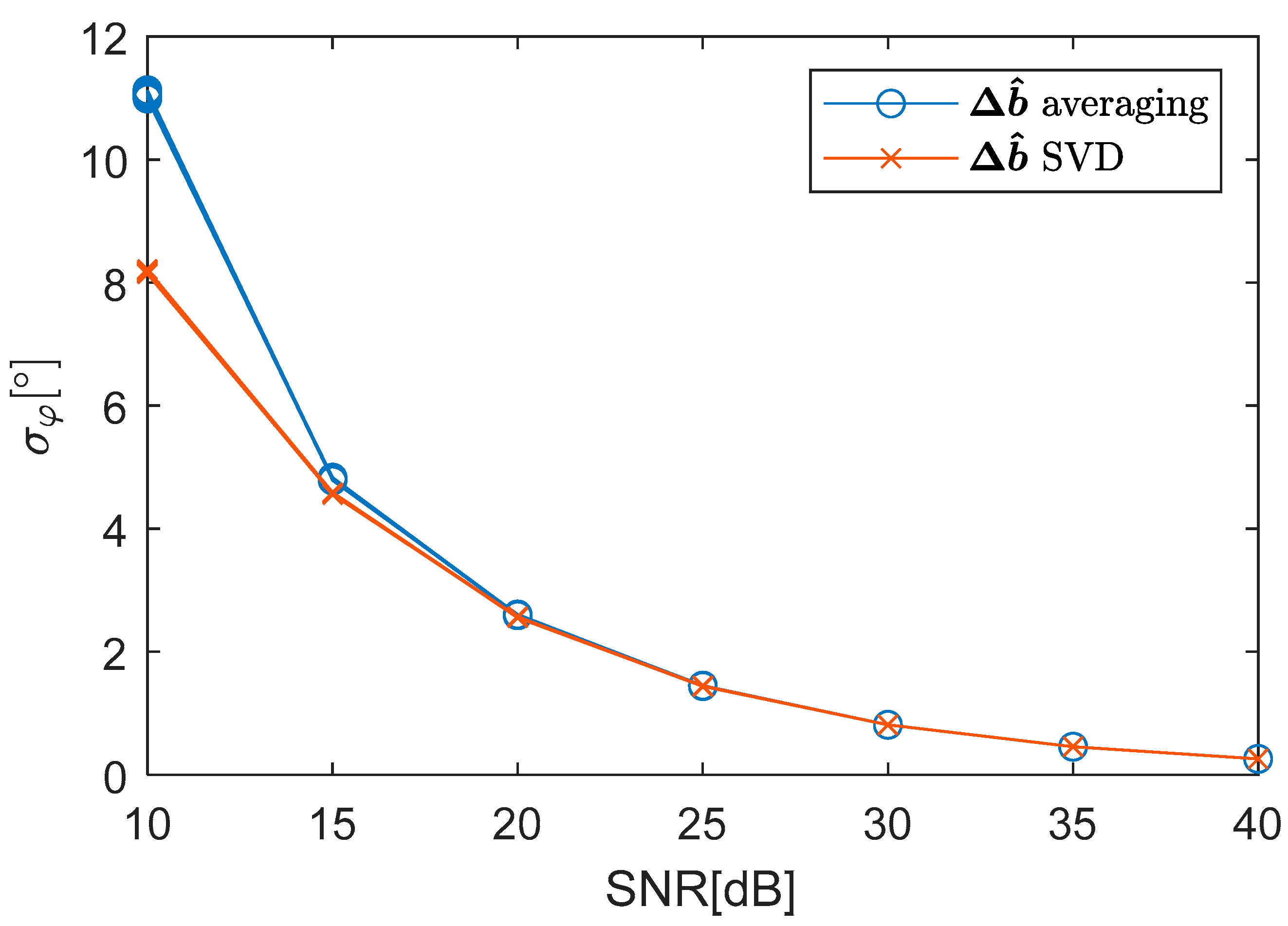
A set of $N={10}^5$ repeated experiments was conducted for each SNR value. In each repetition vectors $\mathsf{\Delta }\widehat{\mathit{a}}$ and $\mathsf{\Delta }\widehat{\mathit{b}}$ were extracted using both algorithms. Then, for each vector entry, the standard deviation of the phase was calculated (Figure 6 and Figure 7). Of course, the results for the first entries $\mathsf{\Delta }{\widehat{a}}_1$ and $\mathsf{\Delta }{\widehat{b}}_1$ were zero due to applied normalization, so they were omitted in the plots. It appeared that the results were nearly identical for all other entries within the same vector. In the picture, the results were presented for both algorithms and both vectors. Plots for subsequent vector entries overlay each other.

Both algorithms performed similarly. There is only a slight improvement for the SVD-based calculation in the case of a poor SNR. In practice, calibration using such a low post-integration SNR is rather not recommended, but if that is the only possibility, the SVD-based method should be chosen.

When the results for both vectors are compared, it is visible that the outcome for vector $\mathsf{\Delta }\widehat{\mathit{a}}$ is better. It can easily be explained with the fact that to calculate each entry of $\mathsf{\Delta }\widehat{\mathit{a}}$ there were 20 combinations with receiving array elements, so there was more excessive information. For each element of $\mathsf{\Delta }\widehat{\mathit{b}}$, only 10 combinations with transmit array elements were available. If the arrays were bigger, the accuracy gain would be even higher.

5. Numerical Evaluation of Channel Array Offsets

In this section, it will be shown that extraction of channel matrix offsets $\mathsf{\Delta }\mathit{A}$, needed for the calibration of MIMO radar, can be improved using the proposed methods. The simulation was performed exactly as in the previous section. This time, the phase standard deviations were calculated for two cases. In one, the offset estimate was taken as the measurement matrix after elementwise normalization by the first entry, according to (14). In the second, the estimate of $\mathsf{\Delta }\widehat{\mathit{A}}$ was obtained from estimated vector offsets

$$\mathsf{\Delta }\widehat{\mathit{A}}=\mathsf{\Delta }\widehat{\mathit{b}}\mathsf{\Delta }{\widehat{\mathit{a}}}^T,$$

(22)

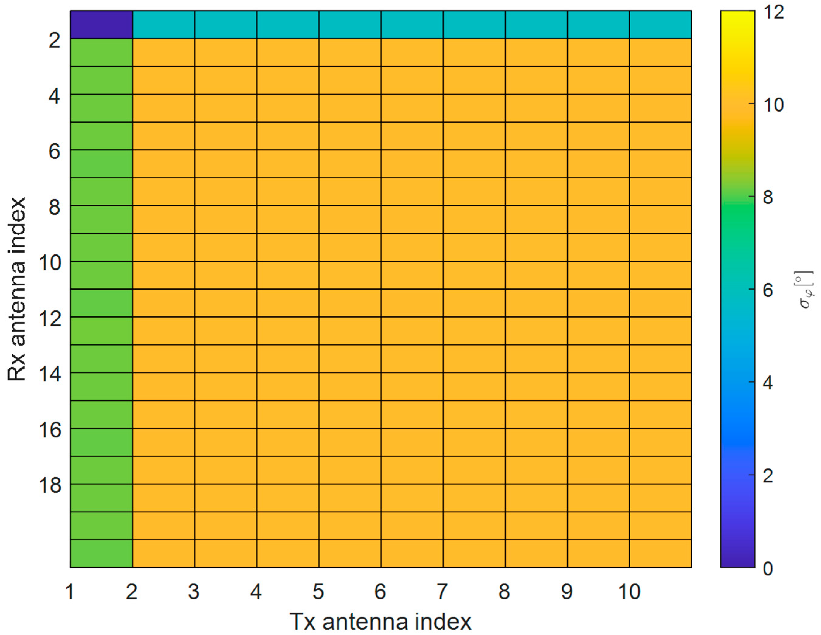
The results are presented in Figure 8. The plots for concurrent matrix entries are overlapped, without discrimination in color. A standard normalization procedure equivalent to the already known method of normalization of virtual array response [9,10] brings the same mean error for each entry, whereas reconstruction from the estimated offset vectors brings three significantly lower levels of error for different matrix entries. The zero error for the reference matrix entry has not been drawn. The fact that there are three different lines for the reconstructed case results from normalization by vectors $\mathsf{\Delta }\widehat{\mathit{a}}$ and $\mathsf{\Delta }\widehat{\mathit{b}}$. To illustrate its origin, a snapshot of angle standard deviation of matrix $\mathsf{\Delta }\widehat{\mathit{A}}$ for an SNR equal to 10 is presented in Figure 9.

The main conclusion, however, is that for the proposed methods, the error is considerably smaller than for simple normalization, and this difference is even more significant for matrix $\mathsf{\Delta }\widehat{\mathit{A}}$ than in the case of vectors $\mathsf{\Delta }\widehat{\mathit{a}}$ and $\mathsf{\Delta }\widehat{\mathit{b}}$, treated separately.

6. Measurement Results

The results were performed using a continuous-wave noise radar demonstrator working in 3 × 3 MIMO mode that was built at Warsaw University of Technology [22]. The size of the array was determined by the available hardware limitations, and it is not big enough to prove the advantage of the proposed methods over simple normalization. The averaging gain for a three-element array does not bring significant improvement. However, the hardware setup is enough to show that the proposed methods work on the experimental data.

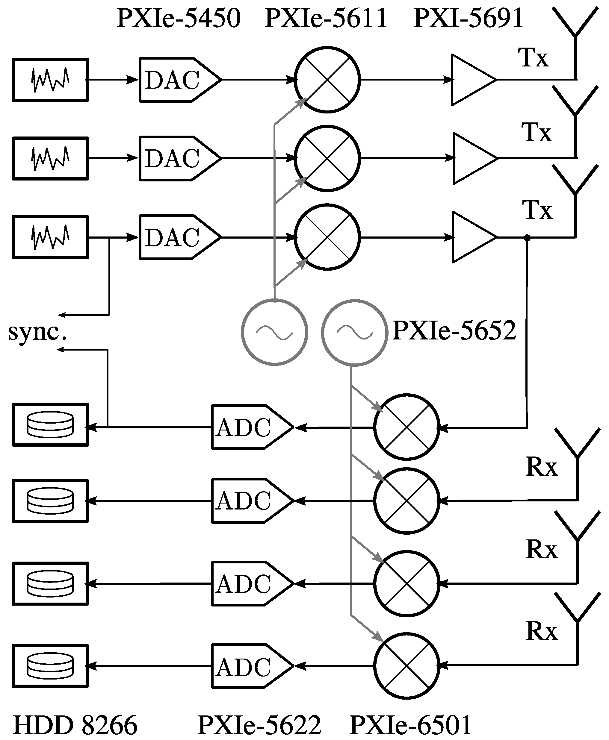
The system was based on COTS modular instruments produced by National Instruments and installed in two PXIe chassis (one for the receiver and one for the transmitter). It used a coherent, multichannel arbitrary waveform generator as a transmitter and a vector signal analyzer as a receiver, with 50 MHz of instantaneous bandwidth. The synchronization between the receiver and the transmitter was possible due to an additional reference channel, a recording signal coupled from one of the transmit channels (Figure 10). The receiver frontend designed for a 2.4 GHz band (λ ≈ 12.5 cm) consisted of a commercial WiFi sector antenna, low noise amplifiers and bandpass filters. Transmit antennas were placed one after another in azimuth, which corresponded to a distance a bit wider than λ/2 spacing between their centers. The transmit antennas were separated by approximately 3/2 λ in a sparse array that together with the receive array constituted a Nyquist MIMO array.

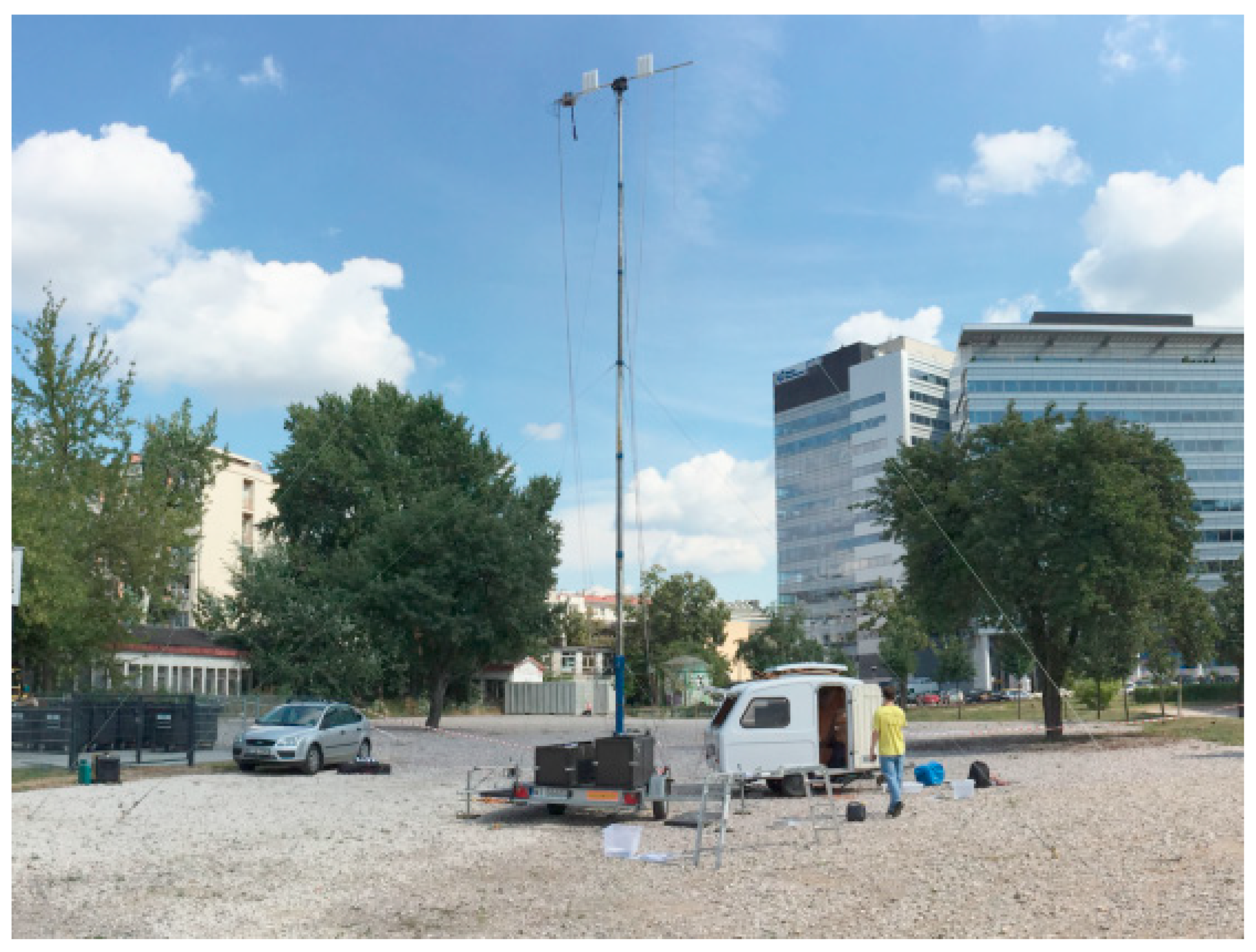
Although the system was phase coherent within a continuous recording, the phase differences induced by cable lengths and initial phases of local oscillators were not compensated by default. This was the motivation for the development of methods described in this paper. As the calibration target, an active echo repeater was used. The repeater was able to introduce a delay and frequency modulation. Especially the false Doppler of the echo allowed one to separate useful calibration from returns from the same range cell but different azimuth angles. Similar calibration performed on a corner reflector did not bring satisfactory results. The radar demonstrator on the test site is presented in Figure 11.

The aim of the experiment was to produce a range-azimuth image of the observed scene within a single integration snapshot. For a MIMO radar, it is possible since both receive and transmit beamforming can be done after signal reception.

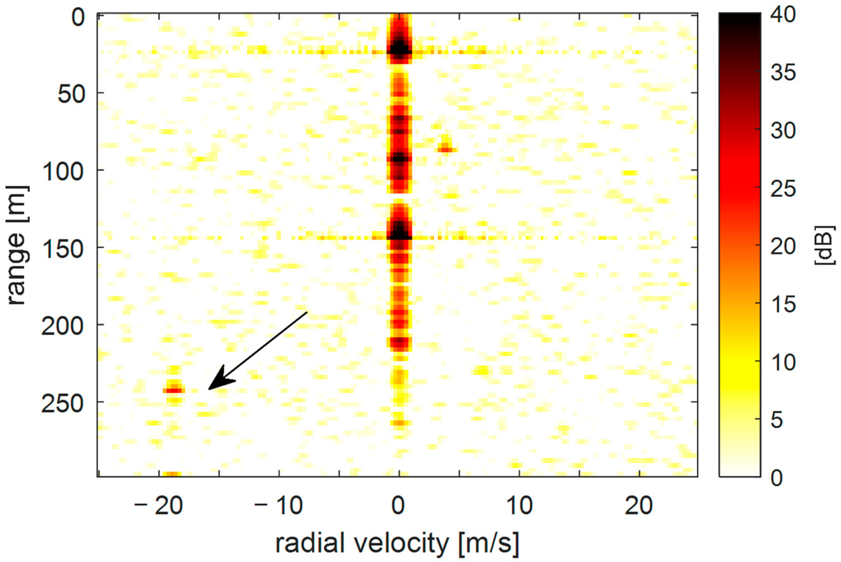
In this case, the preliminary signal processing consisted of the cancellation of direct transmit-to-receive leakage, and the calculation of a set of crossambiguity functions for each transmit–receive antenna pair. An exemplary crossambiguity function is presented in Figure 12. There are stationary echoes at zero velocity, as well as a moving target and repeater echo visible.

The echo of the calibration repeater was then isolated and, using methods developed in this paper, the calibration phase corrections were calculated. The azimuth angle of the repeater was known and the steering vectors toward it were taken into consideration.

To form the image of the observed scene, the vector of the zero Doppler frequency of the crossambiguity functions was taken for each transmit–receive pair (Figure 13). Then, conventional beamforming was done for each range cell. The output was then mapped to the Cartesian plot of response intensity.

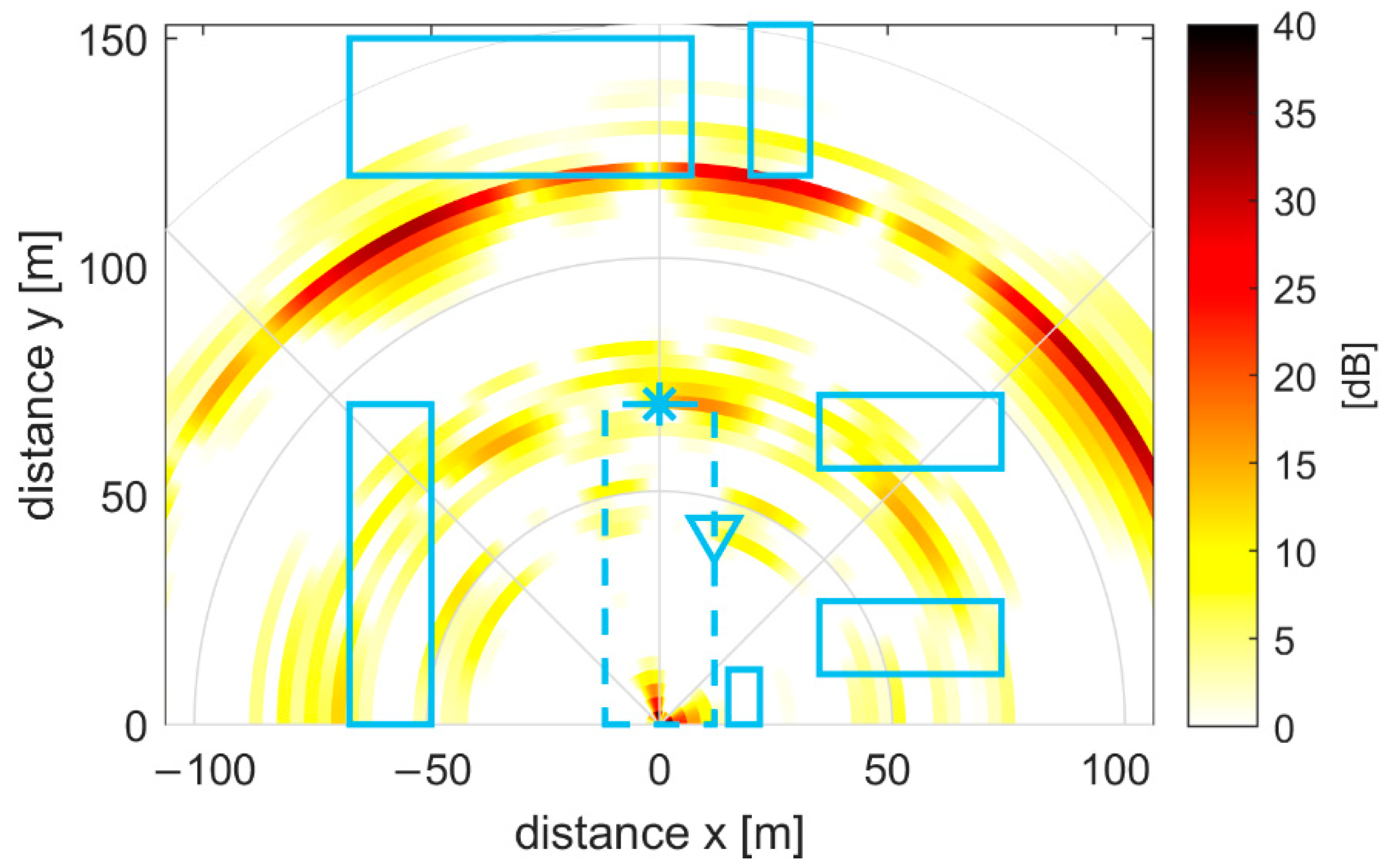
To show the effect of the proposed calibration method, two pictures were produced. One with calibration and one without.

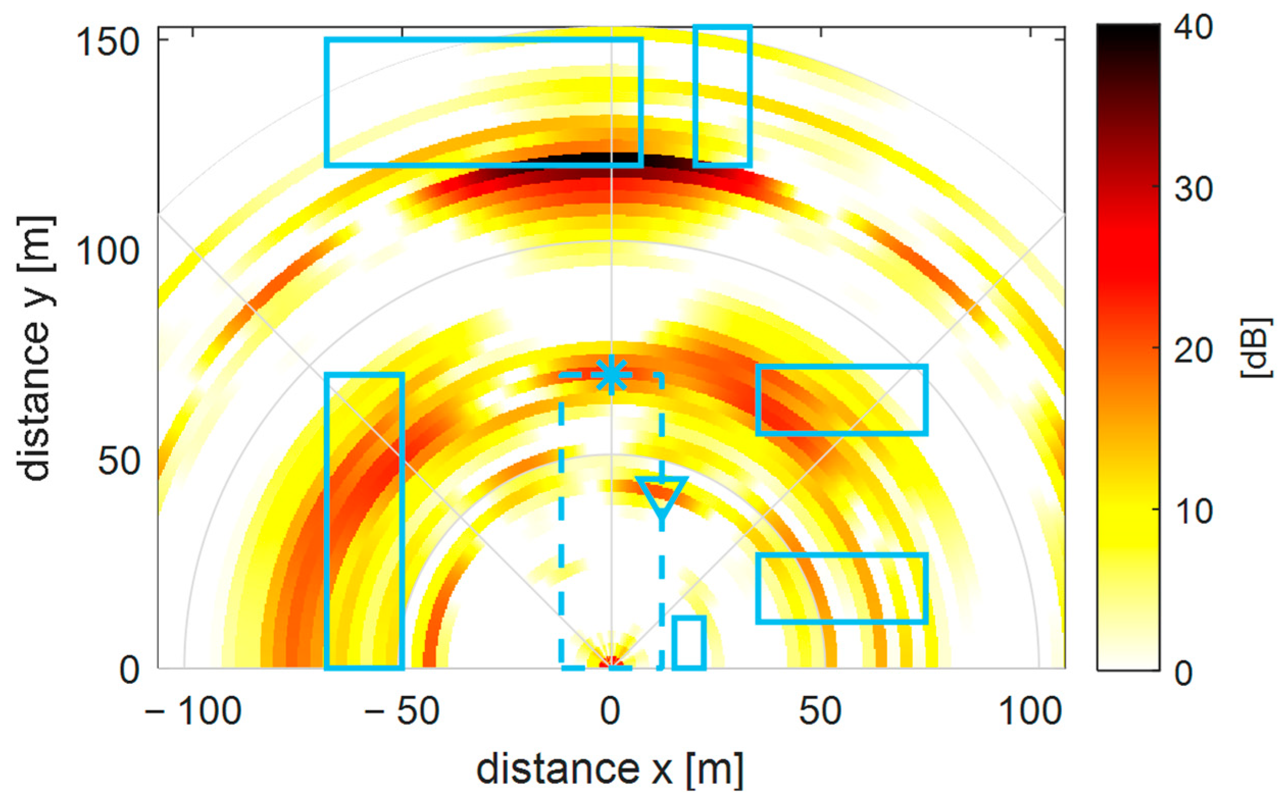
In Figure 14 and Figure 15, the resultant image of the scene is shown. The position of the repeater is marked with a star, the corner reflector with a triangle, and the buildings are represented by rectangles. It can be seen that without calibration there is no echo concentration at the position of the corner reflector. In addition, the echoes of buildings appear at random positions. With calibration, here obtained using the SVD decomposition method, the echo of the reflective horn is clearly visible at the appropriate position, and building echoes match the proper positions. Of course, for a 3 by 3 antenna array the angular resolution is poor, but the experiment undoubtedly shows that single snapshot imaging is possible for MIMO and that the presented method of calibration is effective.

7. Conclusions

The results show that both methods of calibrating phase offsets bring similar results and, due to their simplicity, may have significant practical value. The method using SVD decomposition may have a better performance when the SNR of the calibration target is extremely low. A similar procedure may also be used to mitigate calibration errors in amplitude as well, but for clarity, only phase errors were considered in the paper. This choice has also been driven by the fact that in practice a system has a more stable amplitude between channels than phase. The proposed methods give a better performance than simple normalization of a whole channel matrix by its arbitrary element, which has already been used. The gain in calibration accuracy is better along with the growing number of array elements, but closed form expression for improvement is a matter of further study. The benefit from the proposed methods is that they can be used to retrieve calibration coefficients both for a whole channel matrix as well as separate steering vectors to transmit and receive arrays.