Spatiotemporal Pattern Analysis of Land Use Functions in Contiguous Coastal Cities Based on Long-Term Time Series Remote Sensing Data: A Case Study of Bohai Sea Region, China

Abstract

The long-term accumulated remote sensing data and the emerging cloud-based geospatial processing platform Google Earth Engine (GEE) enable the mining of the spatiotemporal pattern of land-use (LU) functional changes in the contiguous area of large coastal cities. This study proposes a spatiotemporal pattern mining technique for land use function in a large area, which consists of two parts: (1) long-term time series land cover mapping based on the random forest (RF) classification algorithm in the GEE platform and a pixel-by-pixel temporal consistency correction, and (2) spatiotemporal pattern mining based on the constructed spatial temporal cubes (STCs). Specifically, for each LU functional series, we constructed the STC and applied change point detection, time series clustering, and emerging hot spot analysis to mine the spatiotemporal change patterns of LU functions. The study shows that (1) the construction land in the Bohai Sea region from 1990 to 2020 expanded significantly, with the development intensity increasing from 2.08% to 9.77%, having formed a contiguous area of large cities; at the same time, the arable land area decreased significantly, from 57.94% to 47.83%; (2) the emerged construction land experienced three periods: fluctuation, rise, and decline, with 2004 and 2014 being the change points during the period; and (3), the spatial and temporal pattern of the expansion of construction land shows a spatial gradient change in the scale and rate of expansion along the central cities and major axes. This study demonstrates the potential of using long-term time series remote sensing data towards cognizing the generation mechanisms of contiguous coastal big cities.

1. Introduction

The rapid development of externally-oriented economies in coastal countries and regions has led to the high concentration of population and economy in coastal areas and the gradual development of contiguous coastal megacities [1,2]. Monitoring the long-time series changes of land use functions in contiguous areas of large coastal cities serves as an important basis for understanding the mechanisms of change and making policy recommendations to promote sustainable development [3,4,5,6]. Remote sensing has great potential in the fields of coastal zone resource surveying, land use classification, and landscape function monitoring [7,8] because of its wide observation range, abundant spatial and temporal information, and efficient data acquisition method.

The spatiotemporal pattern of land use functional changes mainly relies on the quantity, proportion, and spatial structure of land use [9,10,11]. The typical steps based on the remote sensing technique include classification based on single-time phase images and comparing the classification results of different time phases to obtain change detection information using anniversary dates or anniversary windows (annual cycles or their multiples) [12,13,14]. Due to the large volume of data and the challenges in classification, many studies using term time series of land use have employed time nodes with an interval of three or five years for analysis [15,16,17]. This simplifies the process of data acquisition and analysis, but the possible abrupt change points within the study period may be missed. The newly developed geospatial data analysis cloud platform Google Earth Engine (GEE, https://earthengine.google.com, accessed on 1 May 2022) could help to avoid this oversimplification. With its huge remote sensing image-dataset storage and high-performance computing capability, the GEE provides an efficient way to analyze the land use functional changes in the contiguous areas of coastal megacities [18,19].

Large-scale and long-term time series mapping and change detection for special phenomena using the GEE platform has been applied in construction land expansion [20,21], arable land [22], wetland [23,24], mangroves [25,26], etc. These studies are generally based on time series feature indexes to identify and detect changes in specific phenomena in the coastal zone by reconstructing feature production processes or using time series characteristics such as seasonality and stability. Besides the significant progress in the identification and change detection of time series features, progress has also been made in the detection of long-term time series LU changes in entire elements, including studies at global and regional scales [27,28,29]. Similar studies targeting contiguous areas of large coastal cities have not been intensively explored. Furthermore, the spatiotemporal evolution characteristics of long-term time series images in terms of spatial structure or pattern have not been sufficiently explored, especially not with the help of the spatiotemporal mining methods of long time series.

This study proposes an LU-functional spatiotemporal evolution pattern mining method based on multi-source long-term time series remote sensing data and applies it to the Bohai Sea region of China. It includes (1) a GEE-based method for land use functional classification, whose novelty lies in the pixel-level logical consistency between time and space, and (2) an STC-based spatiotemporal pattern mining method, including change point detection, time-series clustering and emerging hot spot analysis, whose novelty lies in the multi-angle interpretation of the spatial and temporal information behind the data products.

2. Study Area and Datasets

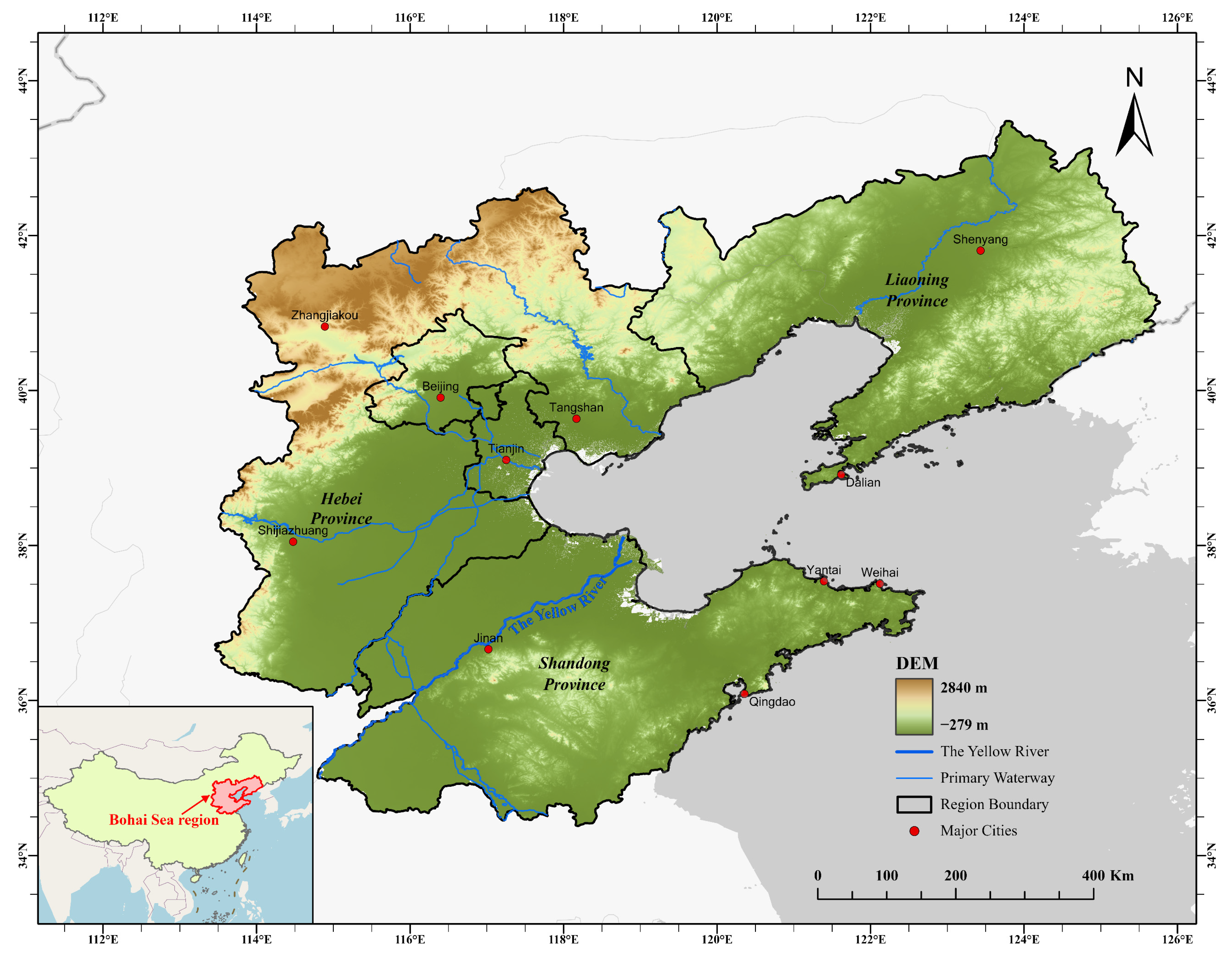
2.1. Study Area

The Bohai Sea region of China includes the vast region surrounding the Bohai Sea and part of the Yellow Sea coast area (34.3°~43.5°N, 113.4°~125.8°E), with an area of 518,000 square kilometers. It encompasses the economic region around the Bohai Sea, with Beijing, Tianjin, and Hebei as its core and Liaodong Peninsula and Shandong Peninsula as its two wings, including Shandong province and Liaoning province (Figure 1). According to the seventh national population census of China, the resident population in the Bohai Sea region has reached 254,488,200, accommodating nearly 18% of the entire population with 5.49% of the country’s land area; the regional GDP reached 3.8 trillion yuan, accounting for 28.2% of the country. Most of the Bohai Rim is a low-lying plain, including the North China Plain, the Huang-Huai-Hai Plain, and the Liao River Plain. It is one of the most agriculturally developed regions in China, as it is an important national production base for wheat, mixed grains, cotton, oilseeds, and fruits. It is also the largest industrial intensive area in the country, with several heavy and chemical industrial bases. The coast of the Bohai Sea contains three major bays, Liaodong Bay, Bohai Bay, and Laizhou Bay, constituting the densest port complex in China with more than 40 ports [30,31]. The Bohai Sea region has formed a spatial framework with two municipalities, Beijing and Tianjin, as its center; open coastal cities such as Dalian, Qingdao, Yantai, and Weihai as the fan; and provincial capitals such as Shenyang, Jinan, Shijiazhuang, Taiyuan, and Hohhot as the regional pivot points, constituting the most important city cluster in northern China that integrates politics, economy, culture, and international communication. It plays a pivotal role in agglomerating, radiating, and driving the regional and national economy. With the trend of international economic centers shifting to the Asia-Pacific region, the Bohai Sea region holds great developmental potential. As an important outlet to the sea in Northeast China, North China, and parts of East China, the Bohai Rim takes the lead in foreign trade, and its total foreign trade volume reached 8.14 trillion yuan in 2020, accounting for about 21% of the country. With the Belt and Road initiative’s construction, the revitalization of Northeast China, and the proposition of the Beijing–Tianjin–Hebei integration strategy, the strategic position of the Bohai Sea region is becoming increasingly prominent.

2.2. Multi-Source Datasets

The data used in this study includes the historical image data of the Landsat series on the GEE platform, including the Landsat Thematic Mapper (TM), Enhanced Thematic Mapper Plus (ETM+), and Operational Land Imager (OLI). We used the GEE platform to screen the extant Landsat data in the Bohai Sea region during 1990–2020. The screening conditions include (1) obtaining data for two periods, June to October (lush vegetation period) and November to March (vegetation withering period), and (2) less than 15% cloudiness. Through screening, we obtained a total of 9242 images. At the same time, to obtain as many annual observations as possible with less than 10% cloud cover during the period from 1990–2020, we used pixel-based mosaic image acquisition means to obtain a total of 31 years of low-cloudiness data for the whole area, which is 6 years more than the traditional whole-view mosaic method. Using the Landsat series historical image data, we calculated spectral indices such as the normalized vegetation index (NDVI), normalized building index (NDBI), normalized difference water index (NDWI), etc., which will be involved as feature variables in the subsequent RF classification process. In addition, the data to assist in the classification include Visible Infrared Imaging Radiometer Suite (VIIRS) nighttime light data, Shuttle Radar Topography Mission (SRTM) digital elevation data, and climate data such as precipitation, air temperature, and cumulus temperature. Among them, the VIIRS Nighttime Day/Night Band Composites Version 1 is a monthly average radiometric composite image of nighttime data from the VIIRS Day/Night Band (DNB) to distinguish urban and non-urban areas. The SRTM data were obtained from the U.S. Land Distributed Activity Archive Center and have been populated using other open-source data (ASTER GDEM2, GMTED2010, and NED). The climate data were collected from the FLDAS data, which is known as the Famine Early Warning Systems Network (FEWS NET) Land Data Assimilation System.

3. Methods

This study proposes a spatiotemporal pattern mining technique for land use functions based on the GEE platform and the STCs, which consists of two parts (Figure 2): (1) long-term time series land cover mapping based on the RF algorithm in the GEE platform [32], and then a pixel-by-pixel temporal consistency correction of land use functional changes, and (2) a spatiotemporal pattern mining method based on the STC. For construction land, arable land, and ecological land, the produced long-term time series land use function products are divided and aggregated to construct a suitable STC, and the spatiotemporal change patterns of land use functions are mined using time-series clustering, change point detection, and emerging hot spot analysis.

3.1. Long Term Time Series Land Use Function Classification and Change Detection

In this study, we utilized the GEE platform to classify and detect changes in land use functions in long-term time series images of the Bohai Sea region, which consists of two steps: (1) using the RF algorithm to obtain the initial LU functional classification products and correcting them based on the logical rules of spatiotemporal consistency, and (2) selecting suitable-sized grid cells and tabulating the imaging products to construct the STCs. Based on the generated STCs, we used the SegNeigh algorithm [33] to identify change points and divide the whole study period into different stages.

3.1.1. GEE-Based Long-Term Time Series Land Use Function Classification in Large Regions

First, we developed an LU functional classification system with reference to previous studies [34,35,36], including 6 types of land for cropland, forest, grassland, water, impervious, and bare land. We selected samples manually and conducted four field trips in 2019 and 2020 to understand the characteristics of each type and to select high-quality sample data. With the help of high-resolution images from Google Earth’s historical archives, we obtained 31 years of sample data by backward modification point by point, i.e., we obtained the training sample in 2018, then switched to the historical images in 2017, checked whether the features changed, and provided category replacement and adjustment to the samples. Such a sample selection strategy ensures the continuity and stability of the sample selection process as much as possible. Based on this strategy, we obtained 249 high-quality sample points annually. Among the selected samples, 80% of them were used as training samples and 20% as validation samples. Second, we selected the NDVI, NDBI, and NDWI as feature variables, and formed different combinations with VIIRS night-lighting data and SRTM digital elevation data. By comparing the accuracies of different combinations, we were able to filter out the feature vectors with higher importance. Afterwards, we randomly divided the sample points into a training set and a validation set by proportion to train the RF classifier. Finally, the images were initially classified using the trained RF classifier. In this process, the initial classification results were optimized by continuously adjusting the sample point distribution, feature vector selection scheme, texture, and window size.

Since the initial classification process ignored the intrinsic logic of the land use and land cover (LULC) development and transition, there were still temporal and spatial logical inconsistencies, and we used a bi-directional spatiotemporal consistency detection method to correct them [37]. The method assumes smooth transitions between different LU types and improves the classification accuracy by modifying the intrusive LU type, which destroys the dominant LU type within two sliding time windows of sequential and inverted orders. We detected and corrected the change sequence of LU types pixel by pixel by combining the initial classification results in temporal order. Considering the numerously repeated LU type changes in the study area, we introduced a hash table to map each change sequence to a corresponding key to improve the computational efficiency. The combined raster is composed of the keys corresponding to the LU type change sequence at their locations. Based on the classification accuracy and the characteristics of the study area, the window size for detection was set as 6 years, and the distribution probability threshold was determined as 0.6. The distribution probability threshold denotes the proportion of dominant LU type in the detection window that is greater than or equal to 0.6. We performed parallel operations on six CPU cores and corrected 389,846 unique LU change sequences in the hash table using a two-way sliding detection window, which took about 20 s to complete. Then, we segmented the image into 12 equal-sized blocks, sliced the corrected sequences behind each pixel in chronological order, and exported the images in chunks year by year from the combined raster. Finally, we mosaiced the exported images by year to produce the ultimate land use functional classification product. It took about 5 h to export and mosaic all the images in chunks.

We selected a 10 × 10 km² grid cell as the analysis unit to perform area segmentation and statistics on the land use functional products and created the STCs. Before that, we categorized the land use functions into three types: construction land, arable land, and ecological land. The ecological land includes forest, grassland, water bodies, and bare land.

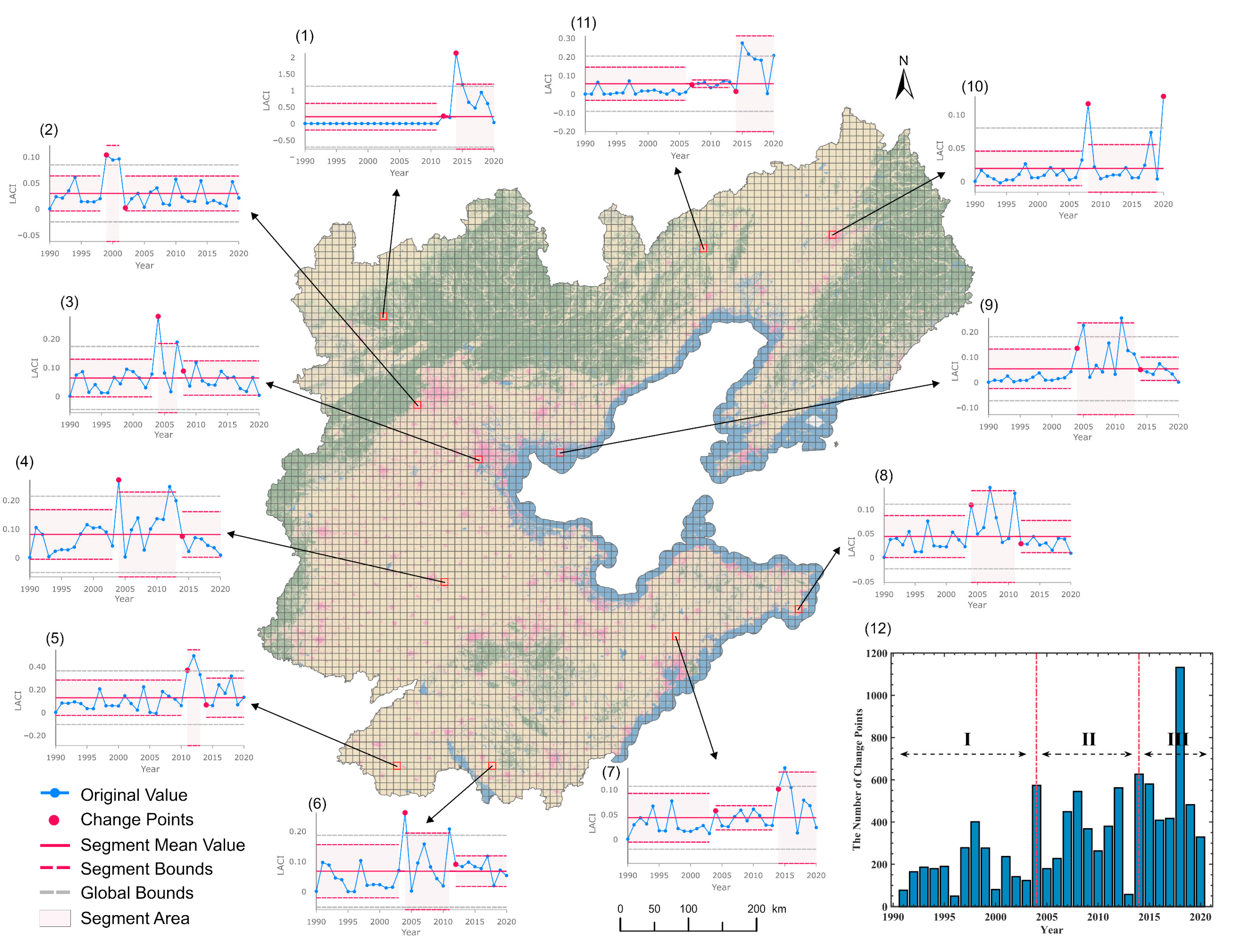
3.1.2. Change Detection Analysis Based on Mutation Points and Rules

The time series of different LU types mostly obey a certain trend and are non-stationary series. The following method was adopted to remove the tendency of the time series. Denote the set of all LU types as $j_{1:v}=\left\{j_1,\dots ,j_v\right\}$, and the set of changepoints as $T_{0:n}=\left\{T_0,\dots ,T_n\right\}$. The area of the $j$th class of features in the $m_{th}$ grid cell in year $t$ can be written as $S_t^{m,j}$. The trend of the series can be removed by subtracting the area $S_t^{m,j}$ at each year $t$($t\in \left(T_0,T_n\right))$ from the previous year $S_{t-1}^{m,j}$, and then taking the logarithm of the difference. The land area change intensity (LACI) between year $t$ and $t-1$ with LU type $j$ in the $m_{th}$ grid can be described as $y_t^{m,j}$ in the following equation.

$$y_t^{m,j}=log\left(S_t^{m,j}-S_{t-1}^{m,j}+1\right)$$

(1)

The reason for adding 1 to the logarithm is to avoid missing values from taking the logarithm when the difference value of the areas is 0.

For the $m_{th}$ grid cell, the time series of its $j$th LU type can be written as $y_{1:n}^{m,j}=\left(y_1^{m,j},\dots ,y_n^{m,j}\right)$. Assume that there are $k$ ordered change points in this sequence, and their position set is ${\tau }_{0:k}=\left({\tau }_0,\dots ,{\tau }_{k+1}\right)$, where $k\in \left[1,n-1\right]$, ${\tau }_0=0$, and ${\tau }_{k+1}=n$. The $k$ change points will divide the sequence into $k+1$ segments, where the $i$th segment is $y_{\left({\tau }_{i-1}+1\right):{\tau }_i}^{m,j}$. Consider the minimum cost of partitioning the sequence $y_{1:n}^{m,j}$ containing k change points as $C_{k,n}^{m,j}$; then, $C_{k,n}^{m,j}$ can be given as

$$\begin{array}{c}{C}_{k,n}^{m,j}=\underset{\tau }{\mathit{min}}\left[{\displaystyle {\displaystyle \sum }_{i=0}^k}\mathcal{C}\left(y_{\left({\tau }_i+1\right):{\tau }_{i+1}}^{m,j}\right)\right]\end{array}$$

(2)

where $\mathcal{C}$ is a cost function for a segment, which is commonly expressed as twice the negative log-likelihood.

A key issue in change point detection is to determine the number of change points. When the number of change points is unknown, a penalty is usually introduced to avoid overfitting. However, setting the same penalty for time series in different locations may result in identifying excessive change points in some cases, and it is difficult to set the threshold value independently for each sequence. Therefore, we set a fixed number of change points and applied the SegNeigh algorithm to obtain the change points. The SegNeigh algorithm can find the segmentation with the lowest cost among all potential segments with the specified number of change points, and thus determine their positions [38,39]. The algorithm uses dynamic programming to search the entire segmentation space to solve Equation (2).

In the case of construction land, we set two change points for each of its $y_{1:n}^{m,j}$ sequences. This would divide each sequence into three segments, where the values within each segment have similar standard deviations. To remove the cases of pseudo-change points and to extract more typical change points, we additionally set the following rules:

(i)

If both moments $t$ and $t+1$are identified as change points, only the higher absolute value of $y_t^m$and $y_{t+1}^m$is retained as the only change point in the sequence;

(ii)

If the values of the sequence do not change in all time points, all change points in the sequence are removed.

We applied change point detection to the study area, quantitatively counted the years in which change points occurred, and spatially determined the locations of the grid cells identified as change points in a given year.

3.2. Spatiotemporal Pattern Mining Method Based on Spatiotemporal Cubes

3.2.1. Spatial Pattern Analysis Based on Time Series Clustering

We applied a K-medoids clustering method to mine the spatial patterns of the STCs. K-medoids clustering is a modification of K-means and is widely used for time series clustering. Instead of using the mean point as the center of the cluster, it uses the medoid point present in the cluster to represent it, whose sum of distances to all other points in the cluster is minimal. K-medoids clustering is more robust towards noise and outliers. The Partitioning Around Medoids (PAM) algorithm uses a greedy search method for K-medoids clustering, which is one of its most representative implementations [38]. Since the grid cell area at the boundary of the study region may be smaller than the internal ones, direct calculation using the land area will cause the incomplete grid cell to present the wrong features. Therefore, we used the land area share for the calculation. For a grid cell $m$ with a total area of $S_m$, the area of the $j$th type of land in its year $t$ is noted as $S_t^j$; then, the proportion of land area of this function $p_t^{m,j}$ is

$$p_t^{m,j}=\frac{S_t^j}{S_t^m}$$

(3)

In the measure of similarity of time series, we chose the Euclidean distance to quantify the similarity in time, which is one of the most common distance measures for clustering time series of equal length and one-to-one mapping [39,40]. Let $F_{1:n}^i=\left(F_1^i,\dots ,F_n^i\right)$ denote a time series of length $n$; the distance $dist\left(i,j\right)$ between it and another series $F_{1:n}^j=\left(F_1^j,\dots ,F_n^j\right)$ can be described as the sum of the distances between all corresponding data points in the two series.

$$dist\left(i,j\right)={\displaystyle \sum }_{t=1}^n\sqrt{{\left(F_t^i-F_t^j\right)}^2}$$

(4)

Thus, multiple land use sequences in the same cluster will be as similar as possible at each time step, which helps to efficiently identify locations with similar land use intensities. We applied this method to three different 10 × 10 km² grid cells that record the proportions of areas of different land types.

3.2.2. Analysis of the Evolutionary Pattern Based on Emerging Hot Spot Analysis

Getis and Ord proposed the $G_i^{*}$ statistic to measure the existence of local spatial associations between observations and their surrounding neighbors [41]. Hotspot analysis using Getis–Ord analysis $G_i^{*}$ can identify regions with statistically significant clustering, reflecting the aggregation degree of high-value areas (hot spot) or low-value areas (cold spot) of the spatial variable over the local space [42]. We conducted Getis–Ord $G_i^{*}$ analysis for each cube in two-dimensional space over a year, and then performed the Mann–Kendall (MK) trend test on each calculated Z-score value series in the time dimension to analyze whether there was a spatial pattern of clustering and whether it had a trend over time [43].

The formula for the calculation of $G_i^{*}$ is

$$\begin{array}{c}{G}_i^{*}=\frac{{\sum }_{j=1}^n{w}_{i,j}{x}_j^v-\overline{X^v}{\sum }_{j=1}^n{w}_{i,j}}{S^v\sqrt{\left[n{\sum }_{j=1}^n{w}_{i,j}^2-{\left({\sum }_{j=1}^n{w}_{i,j}\right)}^2\right]}}\end{array}$$

(5)

where: $i$ represents the central grid cell, $j$ is the grid cell in the neighborhood of $i$, $x_j^v$ represents the area of LU type $v$ in $j$, $w_{i,j}$ is the spatial weight (i.e., spatial distance) between feature $i$ and $j$, $n$ is the number of grid cells in the neighborhood, $\overline{X^v}$ is the mean of the area values of type $v$ land in the grid cell in the neighborhood, and $S^v$ is the standard deviation of the area values of type $v$ land in the grid cell in the neighborhood. $\overline{X^v}$ and $S^v$ are calculated by the following equations.

$$\begin{array}{c}\overline{X^v}=\frac{{\sum }_{j=1}^n{x}_j^v}{n}\end{array}$$

(6)

$$\begin{array}{c}{S}^v=\sqrt{\frac{{\sum }_{j=1}^n{\left(x_j^v\right)}^2}{n}-{\left(\overline{X^v}\right)}^2}\end{array}$$

(7)

The MK trend test uses the data sequence order to acquire the variation trend of the long-term data series [44]. The time series of the Z-score of the $v$th class of features in the cube $m$ is denoted as $Z_{1:n}^{m,v}=\left(Z_1^{m,v},\dots ,Z_n^{m,v}\right)$. Then, the statistical variable $Q_n^{m,v}$ of the MK test can be expressed as

$$\begin{array}{c}{Q}_n^{m,v}={\displaystyle {\displaystyle \sum }_{k=1}^{n-1}{\displaystyle \sum }_{j=k+1}^n}sgn\left(Z_j^{m,v}-Z_k^{m,v}\right)\end{array}$$

(8)

where:

$$\mathrm{sgn}\left(x\right)=\{\begin{array}{ccc}1& \mathrm{if}& x>0\\ 0& \mathrm{if}& x=0\\ -1& \mathrm{if}& x<0\end{array}$$

(9)

The variance of $Q_n^{m,v}$ can be written as:

$$\begin{array}{c}\mathit{VAR}\left(Q_n^{m,v}\right)=\frac{1}{18}\left(n(n-1)(2n+5)-{\displaystyle {\displaystyle \sum }_{p=1}^g}{t}_p\left(t_p-1\right)\left(2t_p+5\right)\right)\end{array}$$

(10)

where g is the number of sets with the same variable value, and $t_p$ refers to the number of data points within the $p$th set.

Based on the hotspot Z scores $Z_{1:n}^{m,v}$ and the MK trend test statistic $Q_n^{m,v}$ at different locations, the hot/cold spots in the study area can be further classified into up to 17 categories according to [43]. Some LU categories may only contain part of the hot/cold spot types based on the change rules of their land functions. We applied this method to three different 10 × 10 km² grid cells that recorded areas of different land types.

4. Results and Discussion

4.1. Results

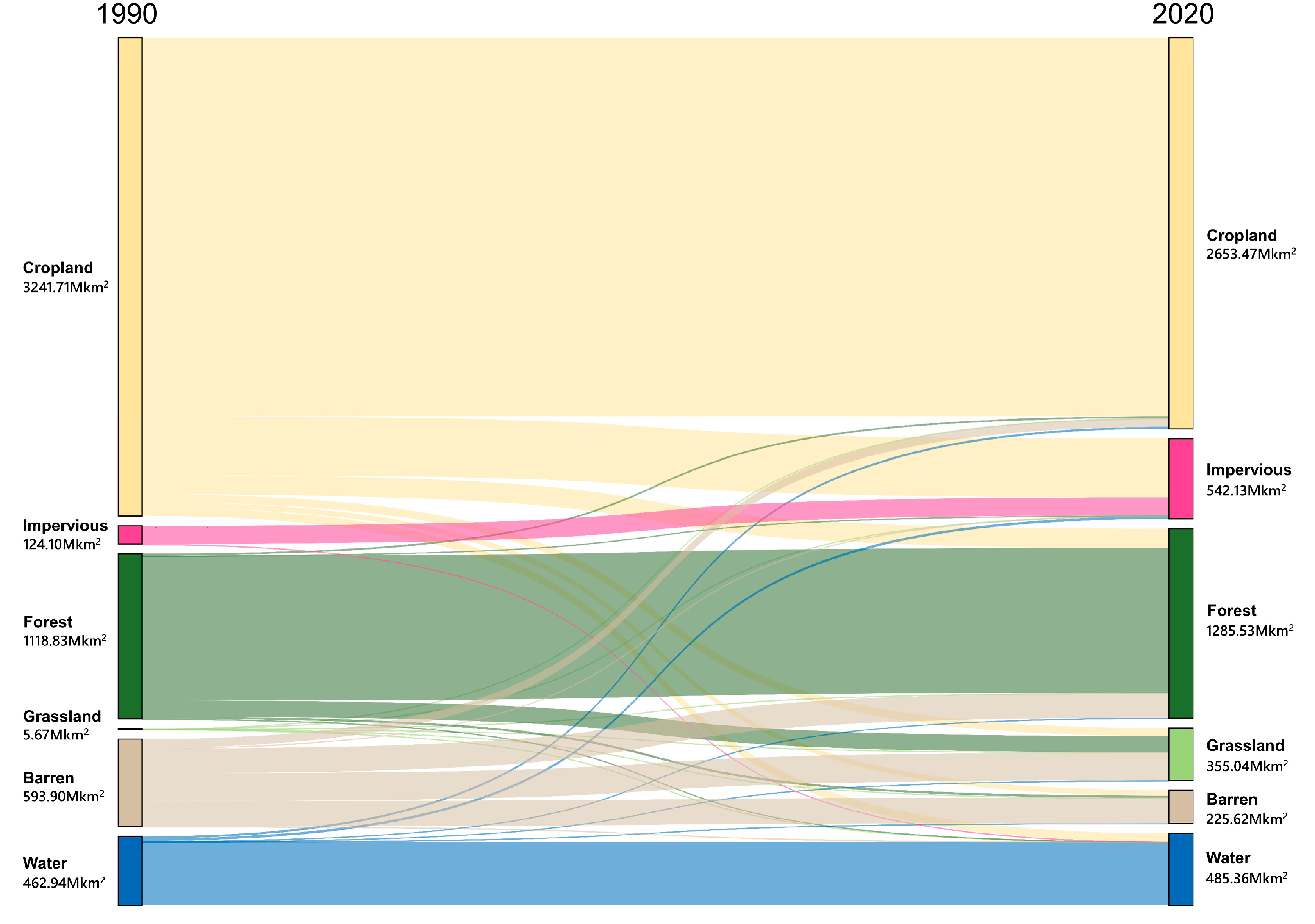
4.1.1. Long Term Time Series Land Use Classification and Change Detection Results in the Bohai Sea Region

After the initial classification and spatiotemporal consistency correction of the long-term time series images, we obtained the ultimate LU functional classification products of the Bohai Sea region (Figure 3). The ultimate classification products achieved high classification accuracy with an average overall accuracy of 95.81% and an average kappa coefficient of 0.94 after evaluation. It is evident that cropland, forest land, and impervious land are the main functional types in the region, and the percentages of these functional lands in 2020 were 47.83%, 23.18%, and 9.77%, which are consistent with the main characteristics of the vast coastal plain area. As is shown by Figure 4, the land types with the most significant changes in the Bohai Rim are cropland, bare land, and forest land. Among them, the conversion of cropland to impervious land is the main type of land use change, with an amount of 39,500 km² (14.08% of the total change area), reflecting the significant impact of urbanization and industrialization. The impervious land transformed from cropland is mainly distributed in central cities such as Beijing, Tianjin, Shenyang, Jinan, and Shijiazhuang; regional central cities such as Zibo, Weifang, and Linyi; and around coastal port cities such as Dalian, Qingdao, and Yantai. This is followed in turn by the transformation of bare land to grassland and cropland to forest land, the figures of which are 18,800 km² (6.70%) and 16,800 km² (6.00%), respectively.

Figure 5 shows the change point detection result for construction land under the 10 × 10 km² grid cell. We calculated the LACI series of construction land for each STC and adopted the SegNeigh algorithm to divide the time series into segments. It is evident from the line graphs that the values in each segment share a similar standard deviation, and the change points are defined as the time step between two segments. The segment bounds indicate two segment standard deviations above and below the global mean with shading, and the global bounds are referred to as two global standard deviations above and below the global mean. It was found that in some ecological areas (Figure 5(1,11)), the LACI of construction land remained at a low value in the early years, and the change points were identified around 2014, reflecting the impact of human activities on the environment. For some inland areas (Figure 5(2–6)), the standard deviation is higher than other stages, which represents the huge impact of urban expansion in this period. In addition, the starting times of urban expansion in different regions are different. This pattern is also well reflected in coastal regions (Figure 5(8,9)). Only part of the situation is listed here. In the vast research area, human activities present diverse patterns of change; therefore, the urban expansion process may be different from the typical pattern mentioned above (Figure 5(7,10)).

By calculating the year-by-year increase or decrease in the total number of change points, we found that the increases in 2004 and 2014 reached 4.67 times and 11 times higher than that of last year, respectively, which are more significant than other years. These two years are important mutation nodes and split the change of construction land into three stages during the 31 years: 1990–2003, 2004–2013, and 2014–2020 (Figure 5(12)). During 1990–2003, the number of change points of construction land in the Bohai Sea region was fluctuating, and the overall trend of change was first to increase and then to decrease. However, the average annual number of change grid cells and the average annual increment of construction land were at low levels, 25.3 and 666.61 km², respectively, and the average annual new construction land per change grid cell was 26.34 km², which was much lower than the last two stages. The number of change grid cells of construction land increased in the second stage and showed a fluctuating upward trend. In addition, the average annual new construction land per change grid cell also reached 34.47 km², an increase of 30.84% compared with the previous stage, which reflects a significant increase in the rate of urban expansion in the second stage. In the third stage, except for a surge in the number of change grid cells in 2018, the overall number of change grid cells of construction land showed a decreasing trend, while the average annual increment of construction land per change grid cell was 39.47 km², a slight increase relative to the second stage.

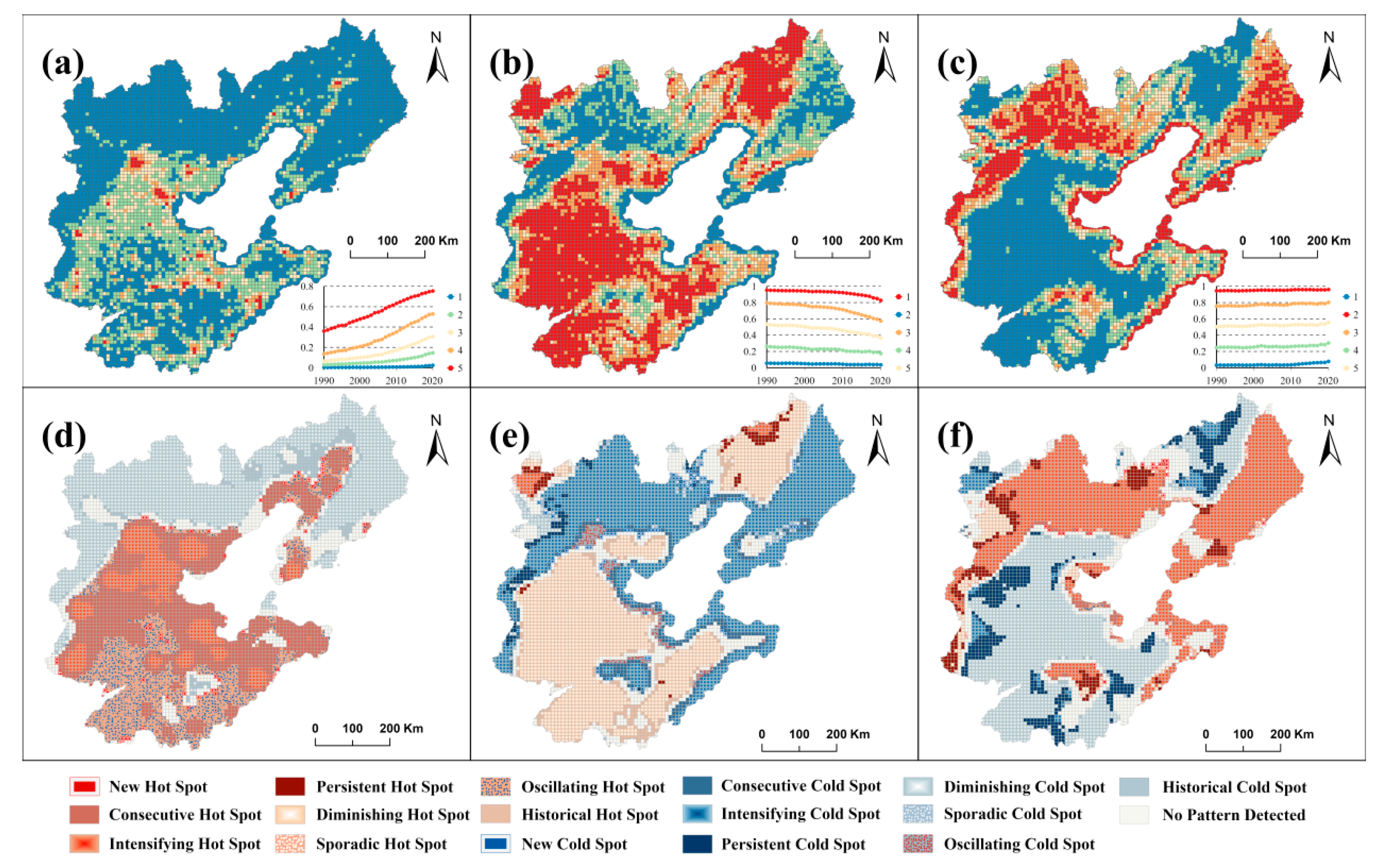
4.1.2. Results of Spatiotemporal Pattern Evolution in the Bohai Rim

To identify the spatiotemporal divergence patterns of construction land, arable land, and ecological land in the Bohai Rim, we conducted time-series clustering and emerging hot spot analyses on construction land, arable land, and ecological land under two 10 × 10 km² grid cells (Figure 6). In the results of the time-series clustering, red (Class I) represents the highest proportion of the corresponding land in the grid cell, followed by orange (Class II) and yellow (Class III), while blue (Class V) indicates the smallest proportion of the land. The percentage of construction land can precisely reflect the development intensity, which can be divided into five categories from high to low: strong (Class I), moderately strong (Class II), medium (Class III), moderately weak (Class IV), and weak (Class V) (Figure 6a). Combined with the line graph of the changes of each type, it is evident that the proportion of construction land shows an increasing trend, among which the more drastic expansion is in the two categories of strong and stronger development grade, and the development intensity of the two categories increased from 37.03% and 14.26% in 1990 to 75.33% and 52.81%, respectively, with an average annual growth rate of more than 1%. These two categories correspond to the main urban areas of each city in terms of spatial distribution, while the yellow (Class III) grid cell with a medium development intensity represents the expansion areas around the prefecture-level cities, and its growth rate is only next to the first two categories, with an average annual growth rate of 0.81%. Arable land, on the other hand, shows an almost opposite spatial and temporal evolution pattern, with an overall decreasing trend, the largest decrease being in Class I and Class II, from 95.04% and 79.09% to 82.68% and 57.31%, respectively. Compared with arable land and construction land, the changes in each classification of ecological land were relatively small and showed an overall upward trend.

Based on the clustering results, we can distinguish the spatial pattern of urban areas in the Bohai Rim as a whole. Overall, it can be divided into three zones: the Beijing-Tianjin-Hebei region, Shandong Peninsula, and Liaodong Peninsula. The Beijing-Tianjin-Hebei region has formed an urban cluster pattern with Beijing and Tianjin as the growth poles and Tangshan as the sub-center, which is echoed by Shijiazhuang in the south of Hebei Province, forming an urban contiguous area. The Shandong Peninsula has formed two city clusters: a coastal belt city cluster with Qingdao as the core, and a provincial capital city cluster with Jinan at its center. The Liaodong Peninsula, on the other hand, forms the Shenyang–Dalian town development axis with Shenyang and Dalian as the core, but in terms of the grid cells with strong and moderately strong development levels, the urban development intensity of the Liaodong Peninsula is slightly lower than that of the Shandong Peninsula and the Beijing-Tianjin-Hebei region. In addition, it is evident from Figure 6a that the distribution of urban clusters in the Beijing-Tianjin-Hebei region and Shandong Peninsula has been transformed from scattered and isolated islands to more closely connected urban contiguous areas, while Liaodong Peninsula is still in a relatively independent state, and its construction land distribution in space is not connected with the Beijing-Tianjin-Hebei region.

The emerging hotspot analysis further demonstrates the pattern revealed by time-series clustering. The dominant hot spot of arable land (Figure 6b) is the Diminishing Hot Spot, which reflects the decreasing clustering intensity of the land categories in the grid cell; the dominant hot spot of ecological land (Figure 6c), which is distributed in the northern part of Beijing-Tianjin-Hebei and the eastern part of Liaodong Peninsula, is the Intensifying Hot Spot. It demonstrates that the clustering intensity and area of ecological land in this region are increasing. The hot spots of construction land are mainly located in the southeastern part of Beijing-Tianjin-Hebei and the northern part of Shandong Peninsula, which appear as an Intensifying Hot Spot in the main urban area and a Continuous Hot Spot in the periphery. These two types of hotspots also form a good match with the clustering results in categories I and II, which indicates that the development intensity level of urban contiguous areas in the Beijing-Tianjin-Hebei region and Shandong Peninsula is not only high but was also in an increasing state during the period from 1990 to 2020. The dense hot spots distributed in the central Liaodong Peninsula and southwestern Shandong Province reflect that the clustering intensity of construction land in this region has been fluctuating and the regional urban development is uneven. These are in agreement with the characteristics of the time-series clustering results. However, some hot/cold spots could reveal a more detailed evolutionary pattern in spatial terms in some cases. The clusters from the time-series clustering results may show more diverse high and low value aggregation characteristics in the corresponding hot/cold spot analysis results, such as the continuous ecological land low value (Class V) area in the middle of the Bohai Sea region, and this low value class is further subdivided into three different types of cold spots, especially in the western part near Shijiazhuang, which shows an aggregation of Persistent Cold Spots and indicates that the ecological land area has a sustained and stable low value level. In conclusion, the emerging hot spot analysis can further complement the fine features of the spatiotemporal pattern.

4.2. Discussion

The STC-based spatiotemporal pattern mining method proposed in this study relies on high classification accuracy and suitably sized grid cells. Previously, the classification of long time-series images tended to ignore the logical consistency of LU evolution among different years. This logical consistency includes not only the similarity in spatial neighborhoods, but also the stability of functional land in time, such as the difficulty of transforming construction land into other types of land. In this study, a bi-directional spatiotemporal consistency detection method was adopted according to the characteristics of a contiguous area with large cities, and the years with a higher overall accuracy were used as the starting and ending points of correction to improve the classification accuracy. The average overall accuracy of the initial classification product is 93.58%, and the counterpart reaches 95.81% after correction, indicating a significant increase of 2.23%. This method was better validated in years with a lower classification accuracy. In five of these years, the overall accuracy improved by over 4%, and this figure further improved by over 3% in more than 1/3 of the period.

We compared the classification quality of our data product with an existing China Land Cover Dataset (CLCD) [45]. We reclassified the shrub land and wetland in the CLCD into forest land and bare land, respectively, to unify the classification system. Then, we used the same sample set for an accuracy evaluation, which found that the average overall accuracy of our corrected data product is about 24.11% higher than that of CLCD, which is a significant increase. Among them, the classification quality of grassland and bare land is significantly better than that of the CLCD, and the accuracy of impervious land and water is also higher in all years. On the one hand, we selected a large amount of high-quality sample points, which were extremely important in the classification process. On the other hand, our classifier pays more attention to the local features of the Bohai Sea region, gaining higher accuracy at the cost of universality. What is noteworthy is that the impacts caused by classification errors in long-term time series change detection are often exponentially cumulative. Therefore, this degree of accuracy improvement is necessary for the subsequent spatiotemporal pattern mining process.

The existence of classification errors at different time nodes with the non-smooth characteristics of different feature time series changes seriously affects the accurate extraction of change points and the recognition of spatial pattern changes. The larger the amount of data, the harder it is to extract the spatiotemporal change features of large regional changes, especially when abstracting the overall pattern of spatial structures. In this process, it is necessary to select appropriate spatial analysis units. This can reduce the influence of classification errors on the one hand and can help to identify the global pattern of spatial structure evolution on the other. After the experiments, we found that a 10 × 10 km² grid cell is a moderate and typical research scale that can capture both the local details of changes and the trends of changes from a global perspective. In addition, we adopted the approach of merging LU classes, such as merging forest, grassland, water, and bare land into ecological land, which weakened the influence of the lower classification accuracy of some LU types to a certain extent.

This study explores the advantages and disadvantages of both the time-series clustering and emerging hotspot analysis methods for identifying spatiotemporal patterns. The time-series clustering method takes a global perspective to match similar patterns in the time series of a certain attribute among all STCs in the region. This method is spatially independent in the process of clustering, without spatial information such as proximity or distance. Therefore, the similarity computed among different regions depends solely on the time series behind them. Compared with time-series clustering, the emerging hot spot analysis additionally considers spatial information. It can capture the similarity degree between an STC and its neighbors in two dimensions, revealing the spatial dependence in an area. It focuses on the question of whether there is a significant agglomeration of land use patterns at a local scale. The calculated temporal trends in emerging hot spot analysis are also different from those of time-series clustering. The temporal trend reflected by the emerging hot spot analysis entails the statistical significance of spatial agglomeration, rather than land use intensity. In contrast, time-series clustering can directly provide the refined change curve behind each cluster and quantitatively show the detailed figures over time.

We conducted multiple sets of experiments based on data characteristics from previous studies and tried different numbers of clusters to test the robustness of the algorithm. We found that the results of clustering for each type of land showed similar trends in overall variation, differing only by orders of magnitude. In the process of land use occupancy in the range of 0–1, setting the number of clusters to five has been sufficient to clearly and comprehensively show the spatial and temporal evolution pattern of the study area, and can effectively identify functional areas such as ecologically fragile areas (cluster 1 and cluster 4 in Figure 6c), rapidly expanding urban areas (cluster 4 and cluster 5 in Figure 6a), and key loss areas of arable land (cluster 3 in Figure 6b). In terms of time-series similarity measurement, besides using Euclidean distance to identify similarity in time, there is another commonly used metric to identify similarity in shape using the DTW (Dynamic Time Warping) distance or statistical correlation. These methods enable us to cluster time series with similar patterns of change and to identify regions with anomalous change locally. In the grid cells selected for this study, the trends of the three LU functions did not differ significantly; therefore, we did not consider identifying the similarity in shape with this metric.

5. Conclusions

Long-term time series remote sensing data facilitate the understanding and monitoring of large-scale surface LU patterns over time. This study not only obtains a long-term time series LU classification product in the contiguous area of large coastal cities with the help of the GEE platform but also explores the spatiotemporal evolution pattern behind it. We found that the LU functions in the Bohai Sea region have changed dramatically in the past 30 years. We delineated three different developmental stages by extracting the change points, and the divergence of each stage is significant. With the help of the time series clustering method and the emerging hot spot analysis method, we uncovered the spatial pattern evolution characteristics implied in the LU classification product, including the global evolution characteristics and local spatial correlation characteristics. The accurate identification of a spatiotemporal pattern depends not only on the classification accuracy but also on the size of the segmented grid cells. Overall, the methods adopted in this study offer great potential towards understanding the processes and mechanisms of the generation and evolution of the contiguous area of large coastal cities, which can provide a fresh perspective for regional macroscopic decision analysis.

References

1. Small, C.; Sousa, D.; Yetman, G.; Elvidge, C.; MacManus, K. Decades of urban growth and development on the Asian megadeltas. Glob. Planet. Chang. 2018, 165, 62–89. [Google Scholar] [CrossRef]
2. Sengupta, D.; Chen, R.; Meadows, M.E. Building beyond land: An overview of coastal land reclamation in 16 global megacities. Appl. Geogr. 2018, 90, 229–238. [Google Scholar] [CrossRef]
3. Gottmann, J. Megalopolis or the urbanization of the northeastern seaboard. Econ. Geogr. 1957, 33, 189–200. [Google Scholar] [CrossRef]
4. Tang, G.; Liu, M.; Zhou, Q.; He, H.; Chen, K.; Zhang, H.; Hu, J.; Huang, Q.; Luo, Y.; Ke, H.; et al. Microplastics and polycyclic aromatic hydrocarbons (PAHs) in Xiamen coastal areas: Implications for anthropogenic impacts. Sci. Total Environ. 2018, 634, 811–820. [Google Scholar] [CrossRef]
5. Yim, J.; Kwon, B.O.; Nam, J.; Hwang, J.H.; Choi, K.; Khim, J.S. Analysis of forty years long changes in coastal land use and land cover of the Yellow Sea: The gains or losses in ecosystem services. Environ. Pollut. 2018, 241, 74–84. [Google Scholar] [CrossRef]
6. Zhang, X.; Song, W.; Lang, Y.; Feng, X.; Yuan, Q.; Wang, J. Land use changes in the coastal zone of China’s Hebei Province and the corresponding impacts on habitat quality. Land Use Policy 2020, 99, 104957. [Google Scholar] [CrossRef]
7. Kulp, S.A.; Strauss, B.H. CoastalDEM: A global coastal digital elevation model improved from SRTM using a neural network. Remote Sens. Environ. 2018, 206, 231–239. [Google Scholar] [CrossRef]
8. Interdonato, R.; Ienco, D.; Gaetano, R.; Ose, K. DuPLO: A Dual view Point deep Learning architecture for time series classification. ISPRS J. Photogramm. Remote Sens. 2019, 149, 91–104. [Google Scholar] [CrossRef] [Green Version]
9. Abdullah, A.Y.M.; Masrur, A.; Adnan, M.S.G.; Baky, M.A.A.B.; Hassan, Q.K.; Dewan, A. Spatio-temporal patterns of land use/land cover change in the heterogeneous coastal region of Bangladesh between 1990 and 2017. Remote Sens. 2019, 11, 790. [Google Scholar] [CrossRef] [Green Version]
10. Sexton, J.O.; Urban, D.L.; Donohue, M.J.; Song, C. Long-term land cover dynamics by multi-temporal classification across the Landsat-5 record. Remote Sens. Environ. 2013, 128, 246–258. [Google Scholar] [CrossRef]
11. Gong, W.; Yuan, L.; Fan, W.; Stott, P. Analysis and simulation of land use spatial pattern in Harbin prefecture based on trajectories and cellular automata—Markov modelling. Int. J. Appl. Earth Obs. Geoinf. 2015, 34, 207–216. [Google Scholar] [CrossRef]
12. Coppin, P.R.; Bauer, M.E. Digital change detection in forest ecosystems with remote sensing imagery. Remote Sens. Rev. 1996, 13, 207–234. [Google Scholar] [CrossRef]
13. Griffiths, P.; Hostert, P.; Gruebner, O.; Van Der Linden, S. Mapping megacity growth with multi-sensor data. Remote Sens. Environ. 2010, 114, 426–439. [Google Scholar] [CrossRef]
14. Schneider, A. Monitoring land cover change in urban and peri-urban areas using dense time stacks of Landsat sat-ellite data and a data mining approach. Remote Sens. Environ. 2012, 124, 689–704. [Google Scholar] [CrossRef]
15. Zhang, Q.; Seto, K.C. Mapping urbanization dynamics at regional and global scales using multi-temporal DMSP/OLS nighttime light data. Remote Sens. Environ. 2011, 115, 2320–2329. [Google Scholar] [CrossRef]
16. Nguyen, L.H.; Joshi, D.R.; Clay, D.E.; Henebry, G.M. Characterizing land cover/land use from multiple years of Landsat and MODIS time series: A novel approach using land surface phenology modeling and random forest classifier. Remote Sens. Environ. 2020, 238, 111017. [Google Scholar] [CrossRef]
17. Wang, J.; Xiao, X.; Qin, Y.; Doughty, Y.B.; Dong, J.; Zou, Z. Characterizing the encroachment of juniper forests into sub-humid and semi-arid prairies from 1984 to 2010 using PALSAR and Landsat data. Remote Sens. Environ. 2018, 205, 166–179. [Google Scholar] [CrossRef]
18. Patel, N.N.; Angiuli, E.; Gamba, P.; Gaughan, A.; Lisini, G.; Stevens, F.R.; Tatem, A.J.; Trianni, G. Multitemporal settlement and population mapping from Landsat using Google Earth Engine. Int. J. Appl. Earth Obs. Geoinf. 2015, 35, 199–208. [Google Scholar] [CrossRef] [Green Version]
19. Liu, D.; Chen, N.; Zhang, X.; Wang, C.; Du, W. Annual large-scale urban land mapping based on Landsat time series in Google Earth Engine and OpenStreetMap data: A case study in the middle Yangtze River basin. ISPRS J. Photogramm. Remote Sens. 2020, 159, 337–351. [Google Scholar] [CrossRef]
20. Liu, C.; Li, W.; Zhu, G.; Zhou, H.; Yan, H.; Xue, P. Land use/land cover changes and their driving factors in the Northeastern Tibetan Plateau based on Geographical Detectors and Google Earth Engine: A case study in Gannan Prefecture. Remote Sens. 2020, 12, 3139. [Google Scholar] [CrossRef]
21. Ye, J.; Hu, Y.; Zhen, L.; Wang, H.; Zhang, Y. Analysis on Land-Use Change and its driving mechanism in Xilingol, China, during 2000–2020 using the google earth engine. Remote Sens. 2021, 13, 5134. [Google Scholar] [CrossRef]
22. Pan, L.; Xia, H.; Yang, J.; Niu, W.; Wang, R.; Song, H.; Guo, Y.; Qin, Y. Mapping cropping intensity in Huaihe basin using phenology algorithm, all Sentinel-2 and Landsat images in Google Earth Engine. Int. J. Appl. Earth Obs. Geoinf. 2021, 102, 102376. [Google Scholar] [CrossRef]
23. Gao, Y.; Cui, L.; Liu, J.; Li, W.; Lei, Y. China’s coastal-wetland change analysis based on high-resolution remote sensing. Mar. Freshw. Res. 2020, 71, 1161–1181. [Google Scholar] [CrossRef]
24. Fekri, E.; Latifi, H.; Amani, M.; Zobeidinezhad, A. A Training Sample Migration Method for Wetland Mapping and Monitoring Using Sentinel Data in Google Earth Engine. Remote Sens. 2021, 13, 4169. [Google Scholar] [CrossRef]
25. Veettil, B.K.; Quang, N.X. Mangrove forests of Cambodia: Recent changes and future threats. Ocean Coast. Manag. 2019, 181, 104895. [Google Scholar] [CrossRef]
26. Zhao, C.; Qin, C.Z. 10-m-resolution mangrove maps of China derived from multi-source and multi-temporal satellite observations. ISPRS J. Photogramm. Remote Sens. 2020, 169, 389–405. [Google Scholar] [CrossRef]
27. Song, X.P.; Hansen, M.C.; Stehman, S.V.; Potapov, P.V.; Tyukavina, A.; Vermote, E.F.; Townshend, J.R. Global land change from 1982 to 2016. Nature 2018, 560, 639–643. [Google Scholar] [CrossRef]
28. Ning, J.; Liu, J.; Kuang, W.; Xu, X.; Zhang, S.; Yan, C.; Li, R.; Wu, S.; Hu, Y.; Du, G.; et al. Spatiotemporal patterns and characteristics of land-use change in China during 2010–2015. J. Geogr. Sci. 2018, 28, 547–562. [Google Scholar] [CrossRef] [Green Version]
29. Zurqani, H.A.; Post, C.J.; Mikhailova, E.A.; Schlautman, M.A.; Sharp, J.L. Geospatial analysis of land use change in the Savannah River Basin using Google Earth Engine. Int. J. Appl. Earth Obs. Geoinf. 2018, 69, 175–185. [Google Scholar] [CrossRef]
30. Zhou, Y.; Kong, Y.; Sha, J.; Wang, H. The role of industrial structure upgrades in eco-efficiency evolution: Spatial correlation and spillover effects. Sci. Total Environ. 2019, 687, 1327–1336. [Google Scholar] [CrossRef] [PubMed]
31. Li, X.; Li, F.; Zhao, N.; Zhu, Q. Measuring environmental sustainability performance of freight transportation seaports in C hina: A data envelopment analysis approach based on the closest targets. Expert Syst. 2020, 37, e12334. [Google Scholar] [CrossRef]
32. Ho, T.K. Random decision forests. In Proceedings of the 3rd International Conference on Document Analysis and Recognition, Montreal, QC, Canada, 14–16 August 1995; Volume 1, pp. 278–282. [Google Scholar]
33. Auger, I.E.; Lawrence, C.E. Algorithms for the optimal identification of segment neighborhoods. Bull. Math. Biol. 1989, 51, 39–54. [Google Scholar] [CrossRef]
34. Han, Z.; Song, W. Spatiotemporal variations in cropland abandonment in the Guizhou–Guangxi karst mountain area, China. J. Clean. Prod. 2019, 238, 117888. [Google Scholar] [CrossRef]
35. Zhang, X.; Zhang, G.; Long, X.; Zhang, Q.; Liu, D.; Wu, H.; Li, S. Identifying the drivers of water yield ecosystem service: A case study in the Yangtze River Basin, China. Ecol. Indic. 2021, 132, 108304. [Google Scholar] [CrossRef]
36. Wu, H.; Lin, A.; Xing, X.; Li, Y. Identifying core driving factors of urban land use change from global land cover products and POI data using the random forest method. Int. J. Appl. Earth Obs. Geoinf. 2021, 103, 102475. [Google Scholar] [CrossRef]
37. Shen, Z.; Wang, Y.; Su, H.; He, Y.; Li, S. A Bi-Directional Strategy to Detect Land Use Function Change Using Time-Series Landsat Imagery on Google Earth Engine: A Case Study of Huangshui River Basin in China. Sci. Remote Sens. 2022, 5, 100039. [Google Scholar] [CrossRef]
38. Kaufman, L.; Rousseeuw, P.J. Partitioning around Medoids (Program PAM). In Finding Groups in Data; John Wiley & Sons, Ltd.: Hoboken, NJ, USA, 1990; pp. 68–125. [Google Scholar]
39. Aghabozorgi, S.; Seyed Shirkhorshidi, A.; Ying Wah, T. Time-Series Clustering—A Decade Review. Inf. Syst. 2015, 53, 16–38. [Google Scholar] [CrossRef]
40. Montero, P.; Vilar, J.A. TSclust: An R Package for Time Series Clustering. J. Stat. Softw. 2014, 62, 1–43. [Google Scholar] [CrossRef] [Green Version]
41. Ord, J.K.; Getis, A. Local Spatial Autocorrelation Statistics: Distributional Issues and an Application. Geogr. Anal. 2010, 27, 286–306. [Google Scholar] [CrossRef]
42. Xu, B.; Qi, B.; Ji, K.; Liu, Z.; Deng, L.; Jiang, L. Emerging Hot Spot Analysis and the Spatial–Temporal Trends of NDVI in the Jing River Basin of China. Environ. Earth Sci. 2022, 81, 55. [Google Scholar] [CrossRef]
43. How Emerging Hot Spot Analysis Works—ArcGIS Pro|Documentation. Available online: https://pro.arcgis.com/en/pro-app/latest/tool-reference/space-time-pattern-mining/learnmoreemerging.htm (accessed on 20 April 2022).
44. Mann, H.B. Nonparametric Tests against Trend. Econometrica 1945, 13, 245–259. [Google Scholar] [CrossRef]
45. Yang, J.; Huang, X. The 30 m Annual Land Cover Dataset and Its Dynamics in China from 1990 to 2019. Earth Syst. Sci. Data 2021, 13, 3907–3925. [Google Scholar] [CrossRef]
Figure 1. Overview map of the study area.
Remotesensing 14 03518 g001
Figure 2. The main technical pathway.
Remotesensing 14 03518 g002
Figure 3. Results of long-term time series land use function classification in the Bohai Sea region.
Remotesensing 14 03518 g003
Figure 4. Sankey chart of different LU functional types from 1990 to 2020.
Remotesensing 14 03518 g004
Figure 5. Change point detection results of construction land under the 10 × 10 km2 grid cell. The line graphs (111) indicate the time-series segment division results in part of the grid cells. The inset at the lower bottom corner (12) shows the distribution of the total number of change points in the whole study area.
Remotesensing 14 03518 g005
Figure 6. Spatial and temporal evolution patterns of land use functions in the Bohai Sea region: (ac) are the results of time-series clustering of construction land, arable land, and ecological land under the 10 × 10 km2 grid cell, respectively; (df) are the results of emerging hot spot analysis of construction land, arable land, and ecological land under the 10 × 10 km2 grid cell, respectively.
Remotesensing 14 03518 g006
Publisher’s Note: MDPI stays neutral with regard to jurisdictional claims in published maps and institutional affiliations.