1. Introduction
It is widely accepted that ecosystems provide multiple benefits for human well-being via ecosystem services (ES). The higher the population density, the more important are the supplies of services, and this is especially the case in urbanized regions. ES provided by the hinterlands surrounding cities, and within cities by green and blue spaces, both have benefits for the urban population [
1]. However, rapid urbanization and population growth can easily lead to the exploitation and degradation of ecosystems [
2], witnessed by findings of the Millennium Ecosystem Assessment [
3,
4], which showed most ES having been in decline over the past years due to human activities [
5]. Specifically, urbanization processes continually shape the quantity and quality of urban blue-green space, determine the location of nature reserves, or, alternatively, influence people’s desires and needs for ES [
6]. Meanwhile, economic growth drivers and policy decisions can also influence management and decision making to change the distribution patterns of ES. The impacts of policies on ES are even more multifaceted and complex. First, policies directly influence the direction of urban development and the balance between economic and ecological priorities. Additionally, regions at different stages of development have different needs and therefore set different priorities for planning. In this context, the mapping and modelling of ES have become an important way to help scientists, managers, and policymakers better understand and manage urban ecological resources, which will further contribute to the restoration of urban ecosystems and the achievement of sustainable development goals (SDGs), especially SDG 11 [
7,
8].
Interestingly, the way in which policies affect urban ES differ substantially between China and Europe. China has experienced rapid urbanization over the past four decades, with its urban population increasing from 170 million in 1978 to 837 million in 2018, and its urbanization level (the proportion of the population living in urban areas) has increased from 18% to 60% during this period [
9]. According to the United Nations Development Programme (UNDP), China’s urbanization level will reach 70% in 2030 [
10,
11]. In addition to rapid urbanization, China has launched a myriad of sustainability initiatives to promote the transition towards urban sustainable development [
12]. For example, the Beijing Plains Afforestation Program has done a great job of improving air quality, mitigating the urban heat island effect, and preventing soil erosion [
13]. Urban green space is also increasing, with 65% of the 117 medium and large cities in China showing increased greening in their urban centers between 2010 and 2019 [
14]. All of the above studies demonstrate the efforts and efficiency of Chinese policies to restore urban ES.
In Europe, the industrial revolution was the major driver for urbanization processes, and urban agglomerations started as early as the 18th century and have mostly reached a saturation stage. For this reason, Europe has been an urban-centered continent for centuries. The urbanization level in Europe has risen at a much slower pace than in China during the last decades, with World Bank statistics showing a rise from 70.8% in 2000 to 75% in 2020 [
15]. Across European regions, different historical and political contexts have caused a high degree of heterogeneity in urbanization patterns, with a diversity of small and medium-sized cities with low growth patterns and only very few megacities [
16]. European cities have undergone a series of low-density discontinuous developments since the 1950s [
17]. Europe has also had active policies to limit urban sprawl, for example by creating “green belts” around cities to protect urban growth or by defining a thirty-hectare target for sealing surfaces to prevent extreme construction activity and promote urban densification. Despite these policies, urban sprawl continues, and urbanization processes intensify [
18]. Different urban development patterns affect the distribution and dynamics of ES at multiple scales. Therefore, comparing the dynamics of Chinese and European urban ES can better reflect the impacts of different urbanization patterns and stages as well as policy instruments on the development of ES, thus improving our understanding of the coupled social–ecological system relationship. Unfortunately, such comparative studies are sorely lacking.
Scenario analysis can provide a more meaningful theoretical basis and decision reference for balancing economic development and ecological conservation and, therefore, has received increasing attention in urban research [
19]. For example, Liu, et al. [
20] constructed several scenarios covering policy and climate change, including the one-child policy and carbon tax policy, and projected the land use distribution under various scenarios, which evaluated impacts on carbon sequestration, soil conservation, and water yields. Based on the aesthetic value and the recreation value of nature reserves, Qin, et al. [
21] combine social and natural factors from the perspective of ES and select priority protected areas by comparing conservation efficiency under multiple scenarios. Gao, et al. [
22] used a CA-Markov model to analyze the land use and ecosystem service values of Shijiazhuang, China in 2030 under a natural development scenario, farmland protection scenario, and an ecological protection scenario. These studies provide an important reference for future urban land cover and ecosystem service estimation.
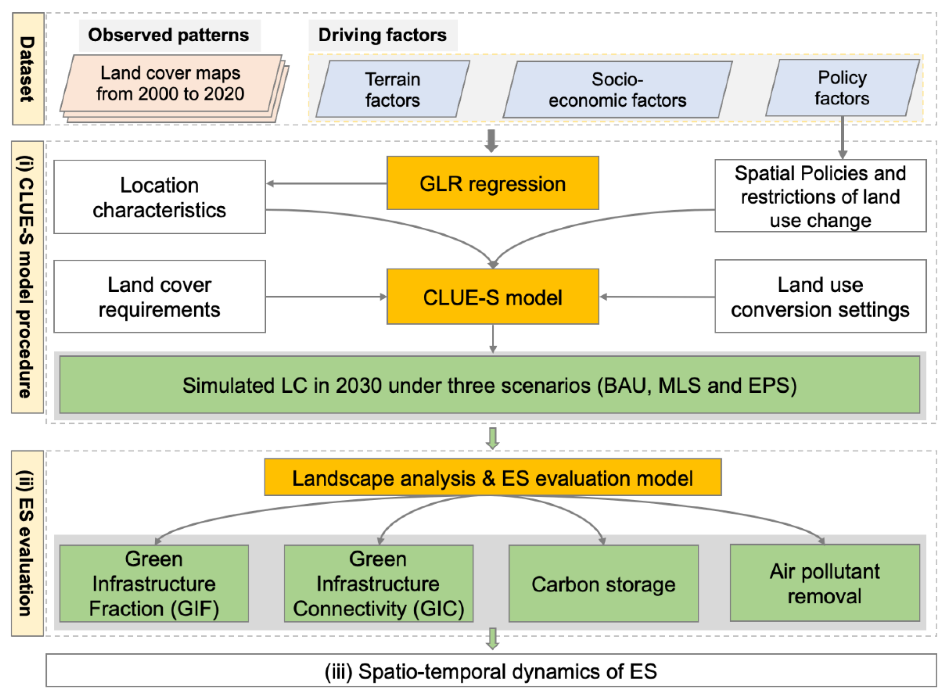
In this paper, our central goal is to understand future urbanization patterns and their effects on ES quantity and equity under a range of policy scenarios. To achieve this goal, the decisive steps towards this are as follows: (1) Predict ES distribution patterns over the next decade under three scenarios. (2) Analyze the differences and characteristics of ES dynamics provided by different phases of development. (3) Explore changes in environmental equity of ES distribution due to urbanization. (4) Assess how land-cover dynamics have led to differences in green infrastructure (GI) and ES changes.
4. Results
4.1. Land Cover Simulation Result
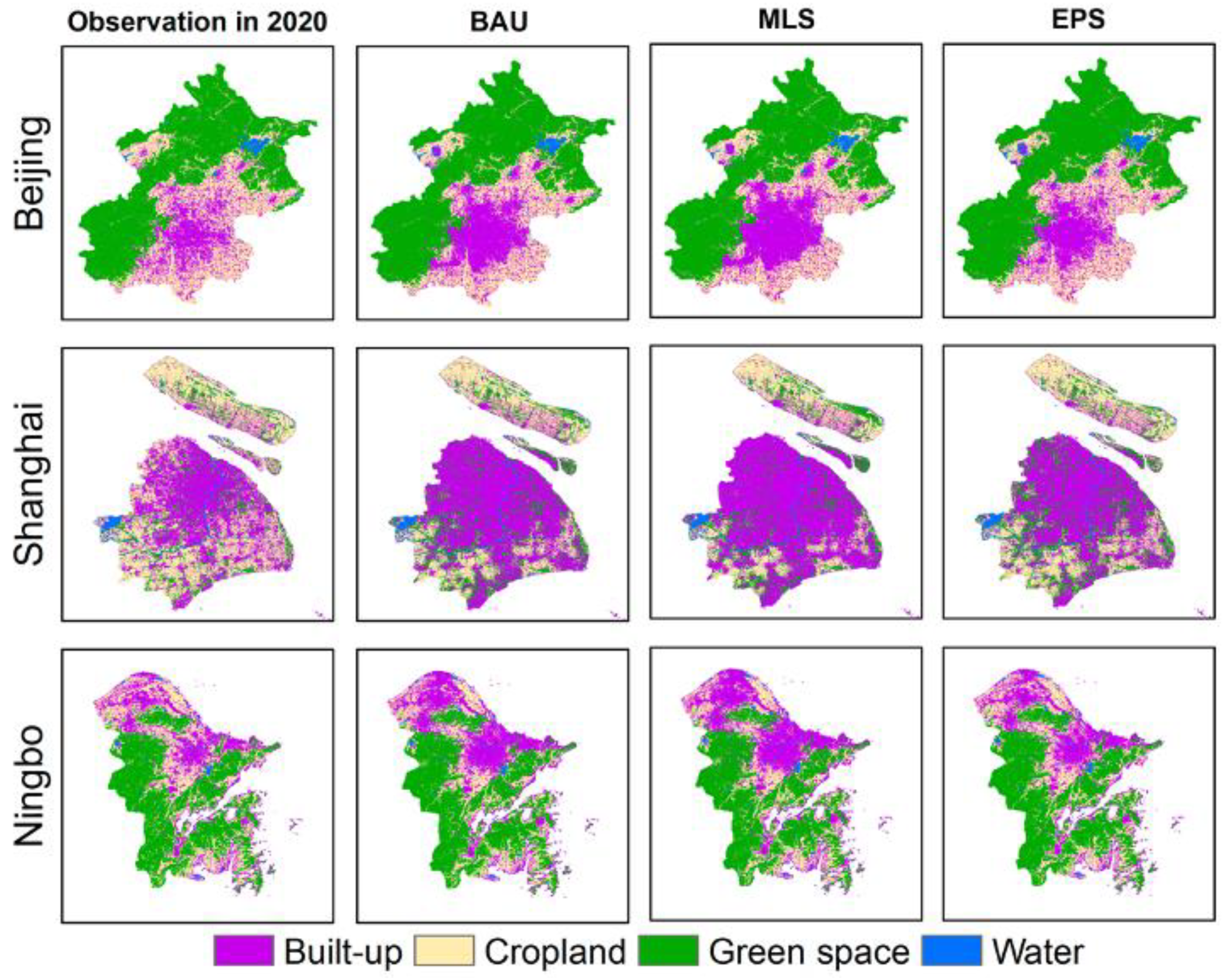
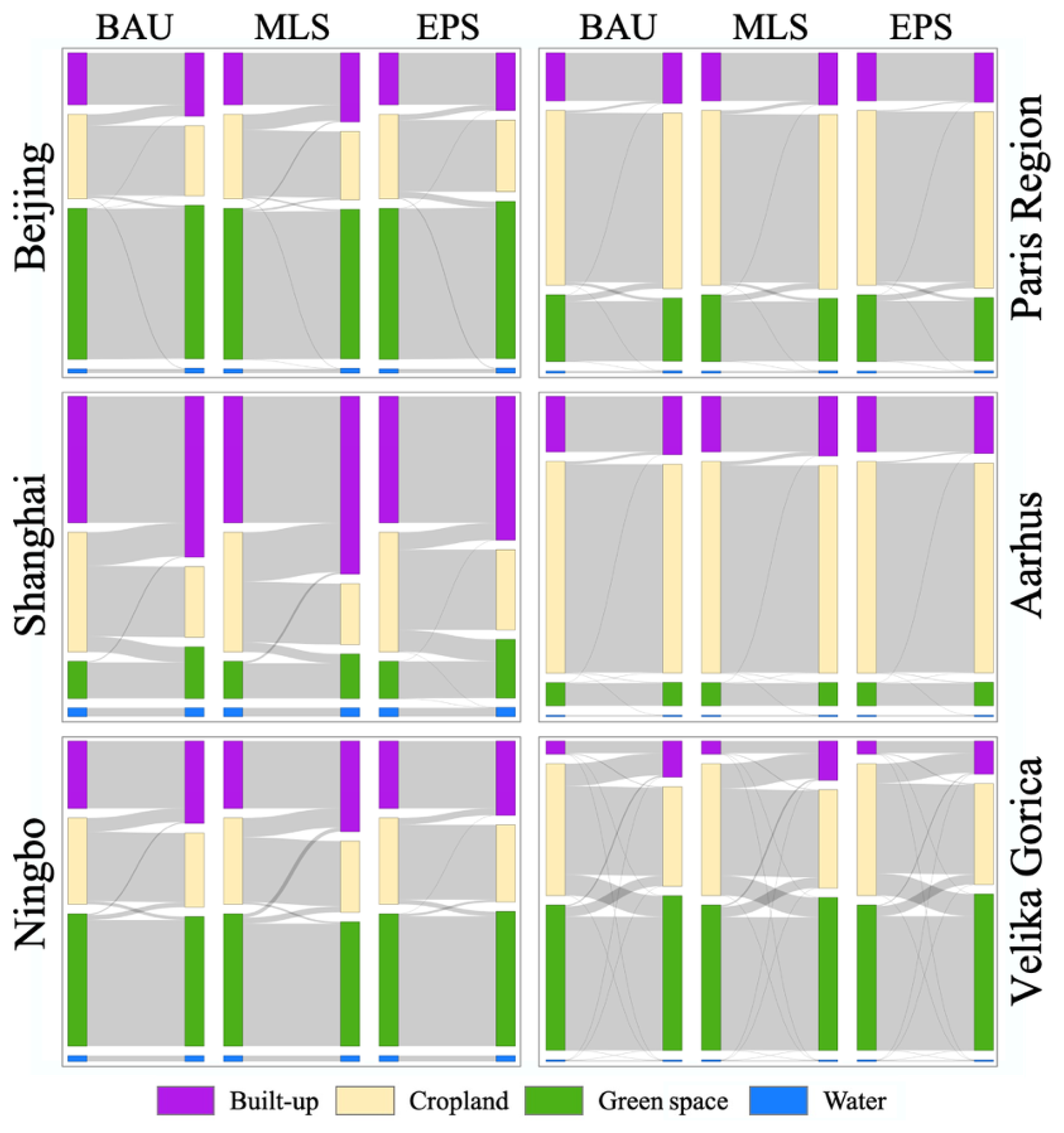
As shown in
Figure 3 and
Figure 4, there is a significant difference between the land cover patterns in 2020 and the three simulated scenarios in 2030.
Figure A2 shows the land cover conversion for different scenarios from 2020 to 2030.
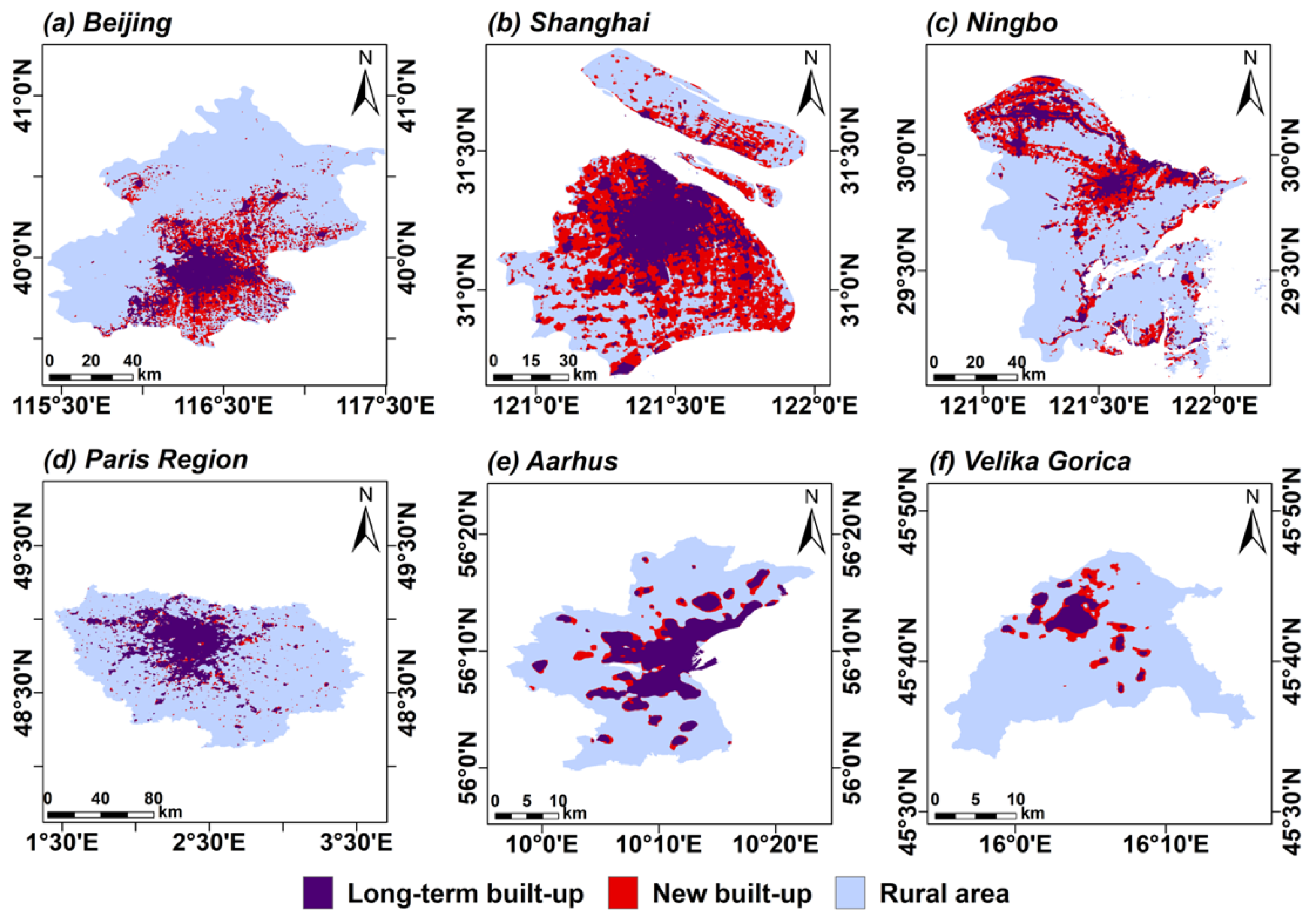
For the three Chinese cities, the built-up area shows rapid growth in all three development scenarios. Specifically, in Beijing, the built-up area grew up to the 643.2 km2 (BAU), 965 km2 (MLS), and 322 km2 (EPS) scenarios by 2030, where almost all (98.7%, 92.3%, and 99.3%) new built-up space was transformed from arable land. In Shanghai, the built-up area increased to 819 km2, 1223 km2, and 413 km2 under the BAU, MLS, and EPS scenarios by 2030. It is worth noting that in all three scenarios in Shanghai, the area of forest grows, mainly converted from cropland, with forest area increasing by 371 km2, 224 km2, and 518.5 km2 in BAU, MLS, and EPS, respectively. In Ningbo, the built-up area increased by 476 km2 (BAU), 720 km2 (MLS), and 215 km2 (EPS). Under the BAU and MLS scenarios, 151 km2 and 189 km2 of forest were converted to cropland, respectively. Overall, the three cities will continue to experience extensive urban expansion in terms of built-up area over the next ten years, with average growth rates of 23.8% (BAU), 35.9% (MLS), and 11.6% (EPS). In the process, cropland will become less available, with average reductions of 24.1% (BAU), 28.6% (MLS), and 19.5% (EPS) in the three cities. The green space area in the three cities shows different trends from 2020 to 2030, with Beijing and Ningbo showing relatively few changes in the green space area under the three scenarios, while in Shanghai, the green space area increases to varying degrees under the three scenarios, at 39.5 km2 (BAU), 19.9 km2 (MLS), and 58.8 km2 (EPS).
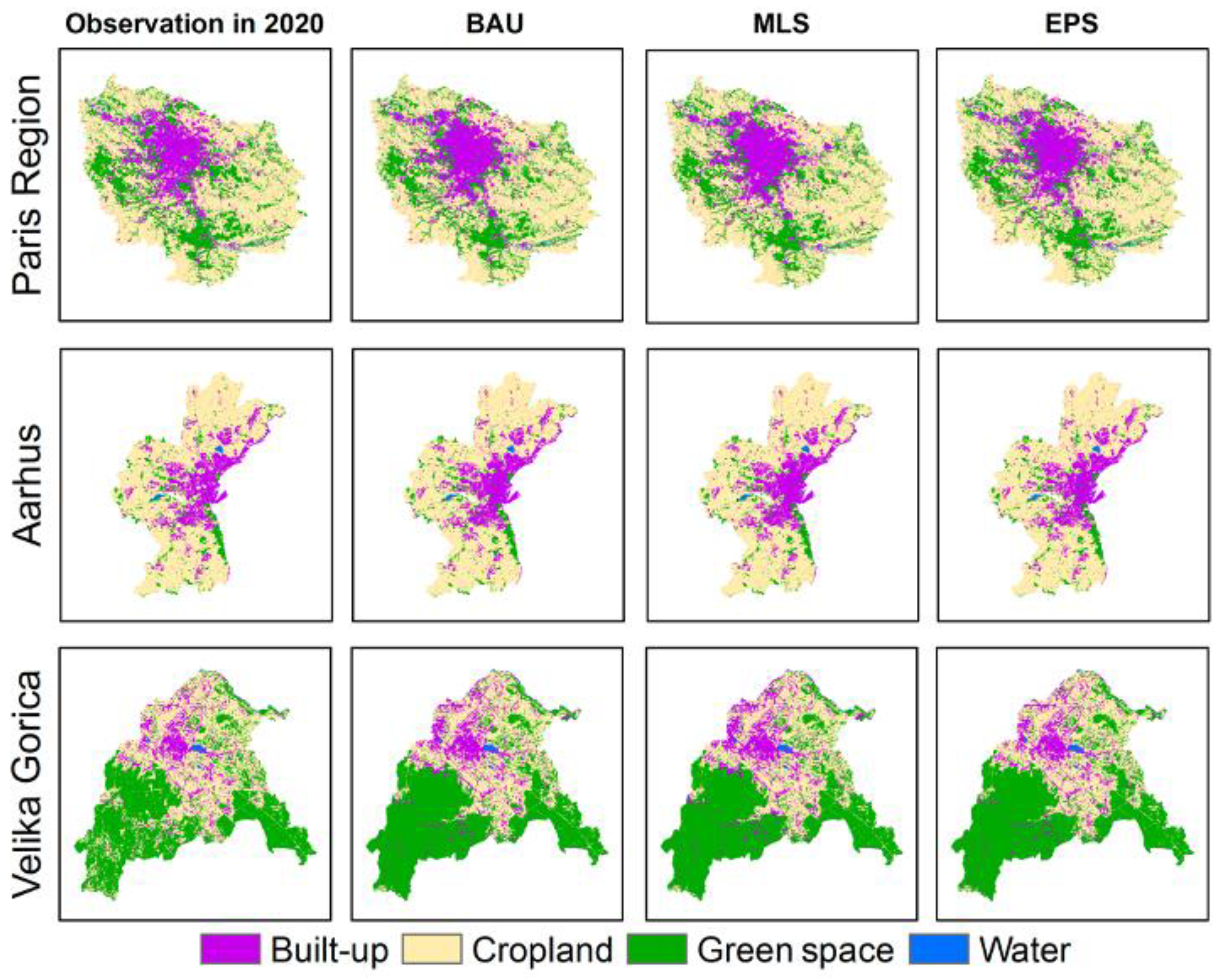
The land-cover patterns of the three European cities for the year 2030 are shown in
Figure 4. The Paris region and Aarhus exhibited relatively little urban expansion between 2020 and 2030, with Paris showing built-up area growths of 111 km
2 (BAU) with a growth rate of 5.5%, 116 km
2 (MLS) with a growth rate of 8.3%, and 56 km
2 (EPS) with a growth rate of 2.8%. Velika Gorica demonstrated a relatively significant urbanization intensity, with built-up area growths of 6.6 km
2 (19.6%) (BAU), 10.1 km
2 (29.9%) (MLS), and 3.1 km
2 (9.3%) (EPS), respectively. The average growth rates of built-up area in the three municipalities range from 10% (BAU) to 15.2% (MLS) and then drop down to 5% (EPS). The average decreases in cropland area are 6.8% (BAU), 7.6% (MLS), and 6.1% (EPS). There are differences in the trends of green space in the three cities: specifically, the green spaces in Aarhus and Velika Gorica show an increasing trend, while the area of green space in the Paris region decreases in all scenarios, with decreases of 5.3% (BAU), 5.9% (MLS), and 4.8% (EPS).
For the validation of land-cover simulation results,
Table A2 shows the ROC values of the logistic regression results. The mean value of ROC for each land cover was greater than 0.8 across all six cities, indicating a good correlation and ability to explain land cover based on the selected driving factors.
Table A3 shows the evaluation of the classification results for the six cities obtained by comparing the observed and simulated land cover in 2020 using 2000 random samples per city, where the mean value of the overall accuracy reached 0.8 and the mean value of the kappa value was 0.74 (
Table A3). These figures indicate that the land-cover simulation model developed in this study can produce a convincing result.
4.2. Dynamics of GI and ES
4.2.1. GI Fraction and Connectivity Changes
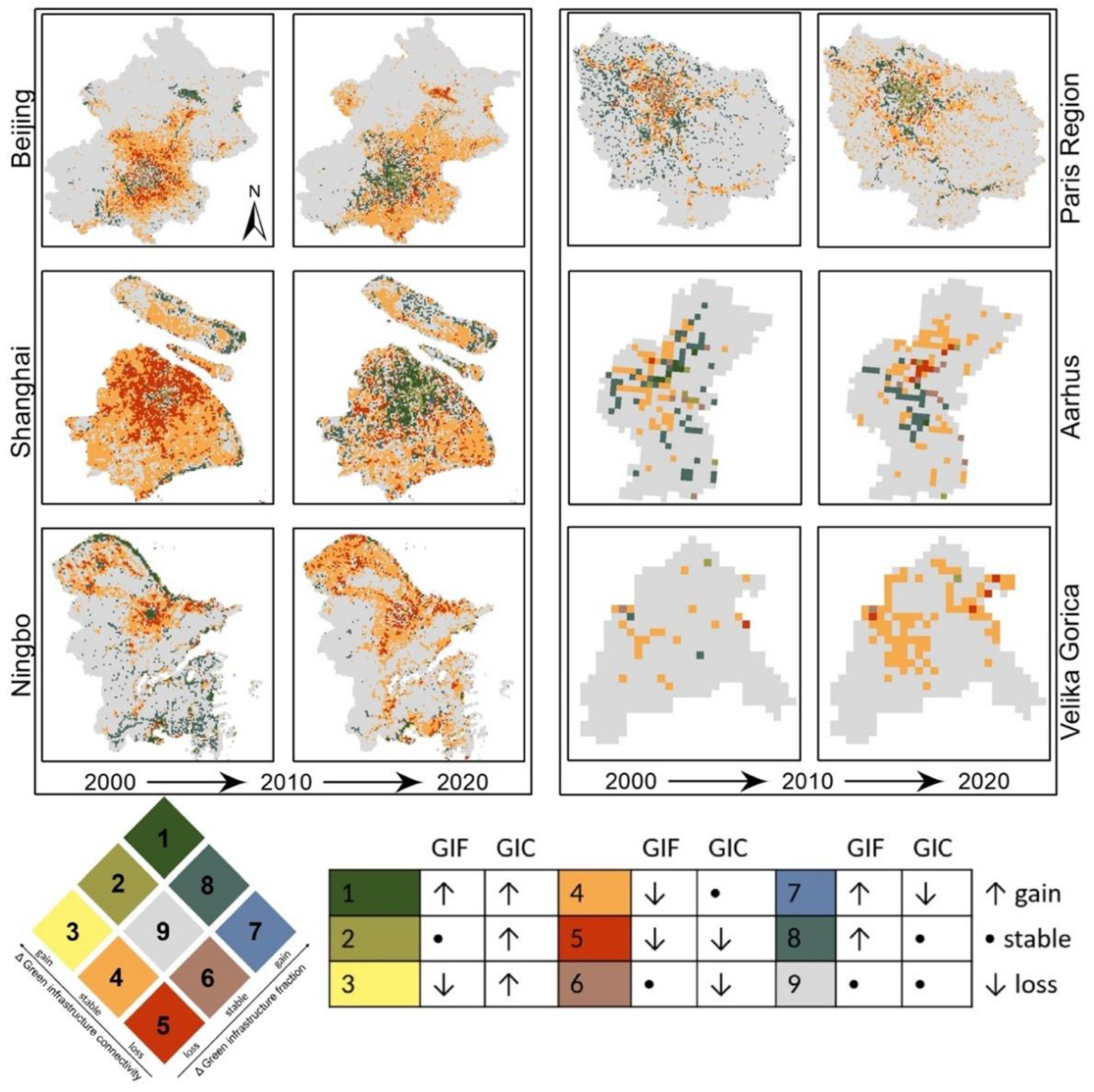
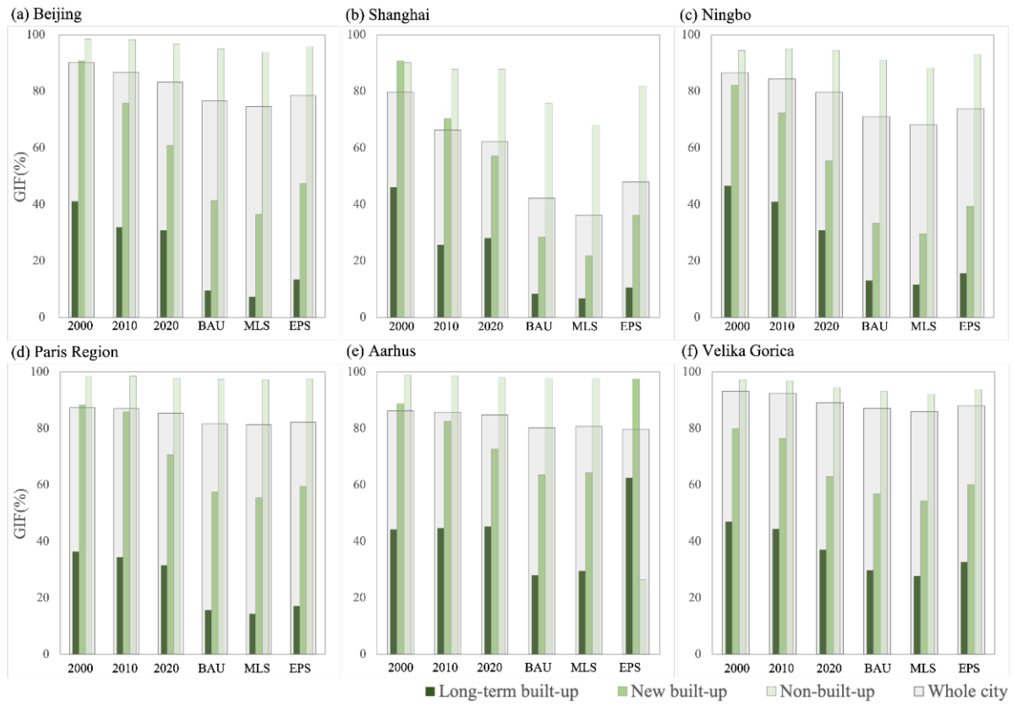
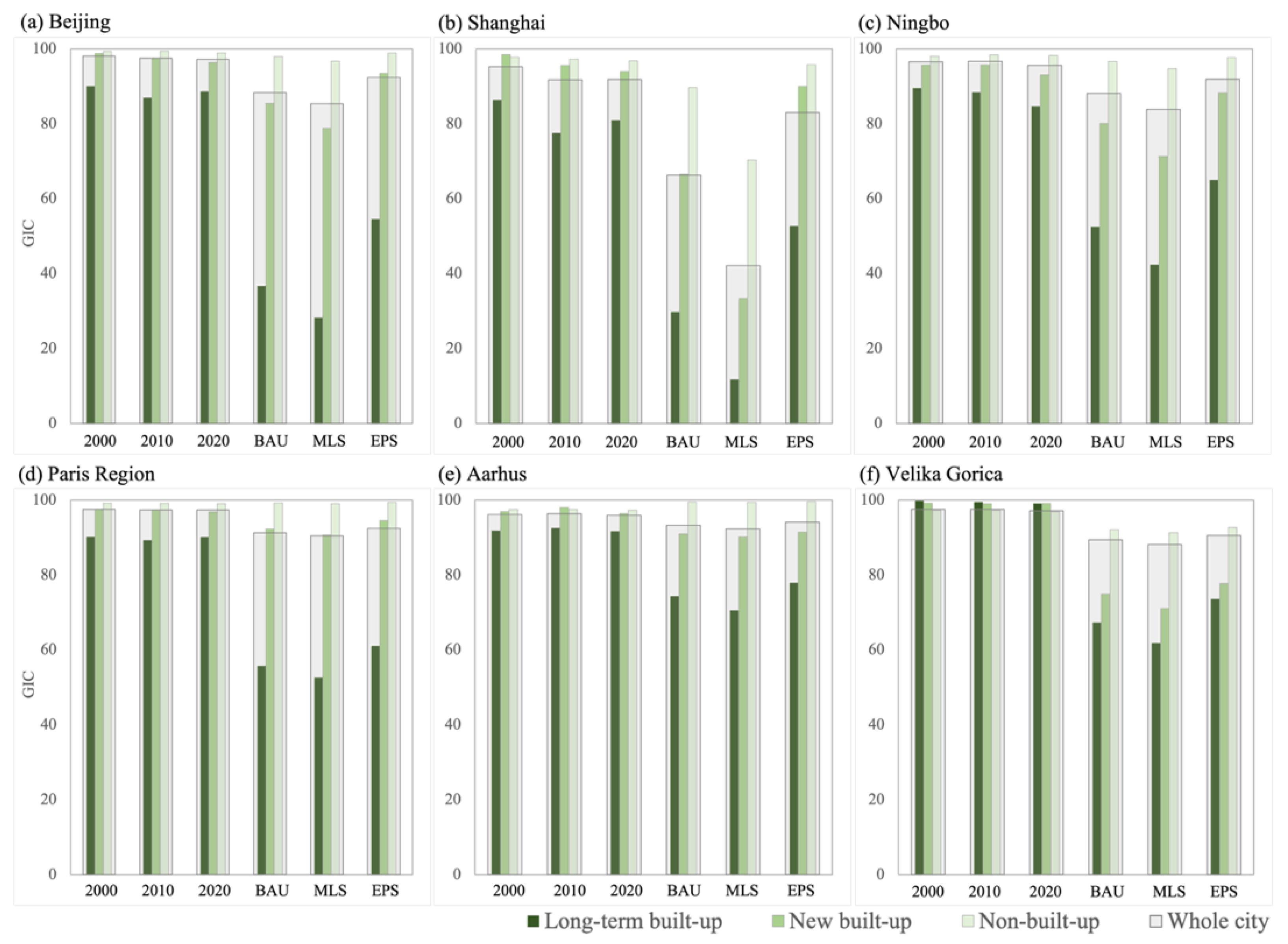
Figure 5 shows the changes in GIF and GIC distribution for the six cities from 2000 to 2020. At the city-wide scale, the GIF values of the three Chinese cities decrease significantly; the average of GIF in the three cities decreased from 85.5% in 2000 to 75.1% in 2020. The most significant reduction in GIF is in the new built-up area, where the average GIF of the three cities in the region decreases from 88% in 2000 to 57.8% in 2020. It is worth noting that the GIF and GIC values increase for most areas of the long-term built-up in Beijing and Shanghai between 2010 and 2020. It is also reflected in the regional averages; for example, from 2010 to 2020 in Shanghai, the GIF of the long-term built-up region increases from 25.6% to 28.1% and the GIC increases from 77.6 to 81. For the three European cities, the changes in GIF and GIC at the city scale are insignificant, with a slight decrease from 89% in 2000 to 86.4% in 2020 for the three cities. GIF, on the other hand, also shows a very small decrease from 97.1 in 2000 to 96.8 in 2020.
The GIF and GIC in different scenarios in 2030 show a big difference between cities in China and Europe (
Figure 6). In China, the average GIFs for the three cities are 59.7% (MLS), 63.3% (BAU), and 66.8% (EPS). In the EPS scenario, GIF increased by 7.1% relative to the MLS scenario, and GIC increased by 18.7 relative to MLS. In the three European cities, the GIFs were 82.7% (MLS), 83% (BAU), and 83.4% (EPS), and the GICs were 90.3 (MLS), 91.3 (BAU), and 92.3 (EPS), respectively, with small differences across scenarios.
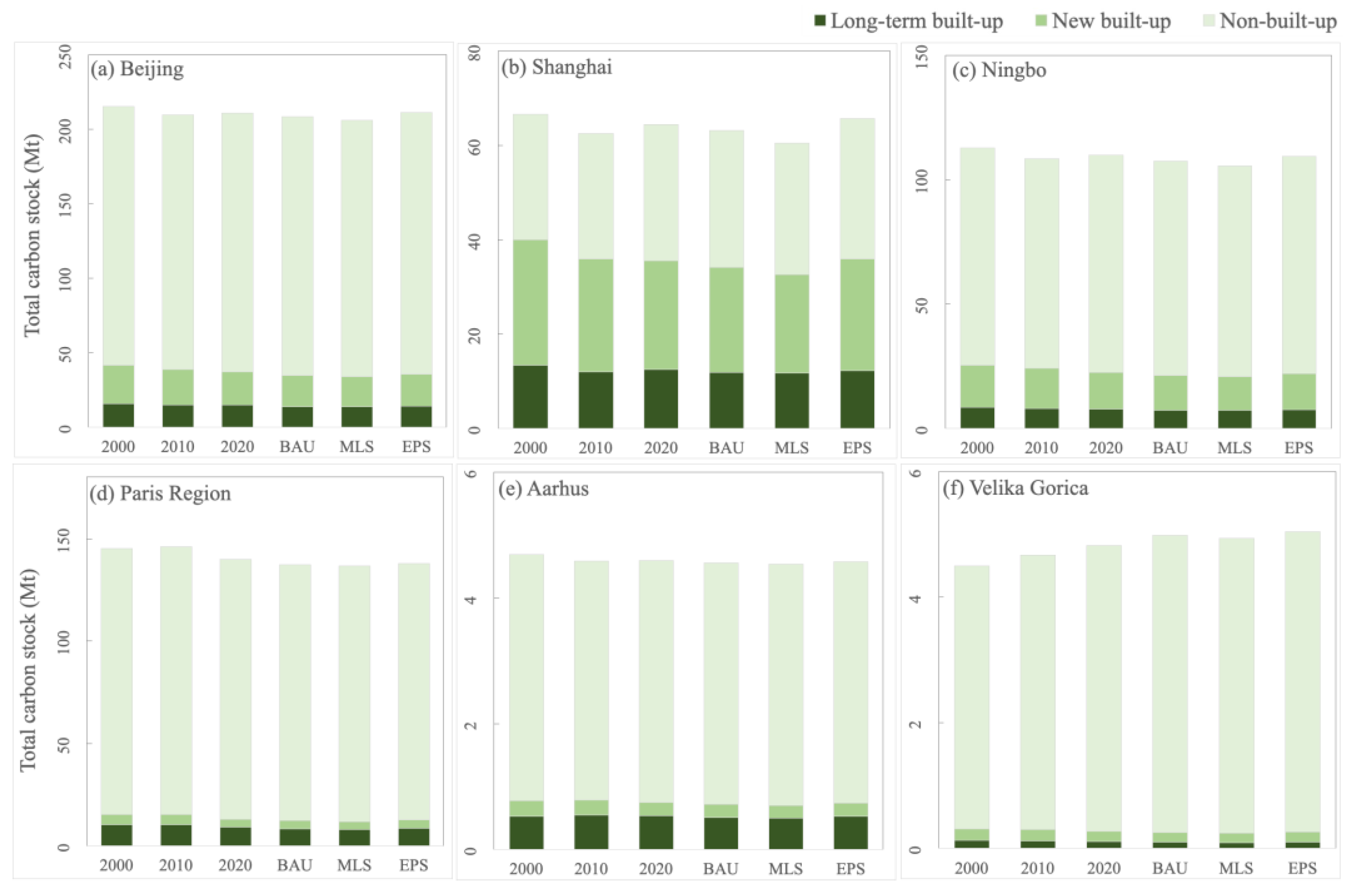
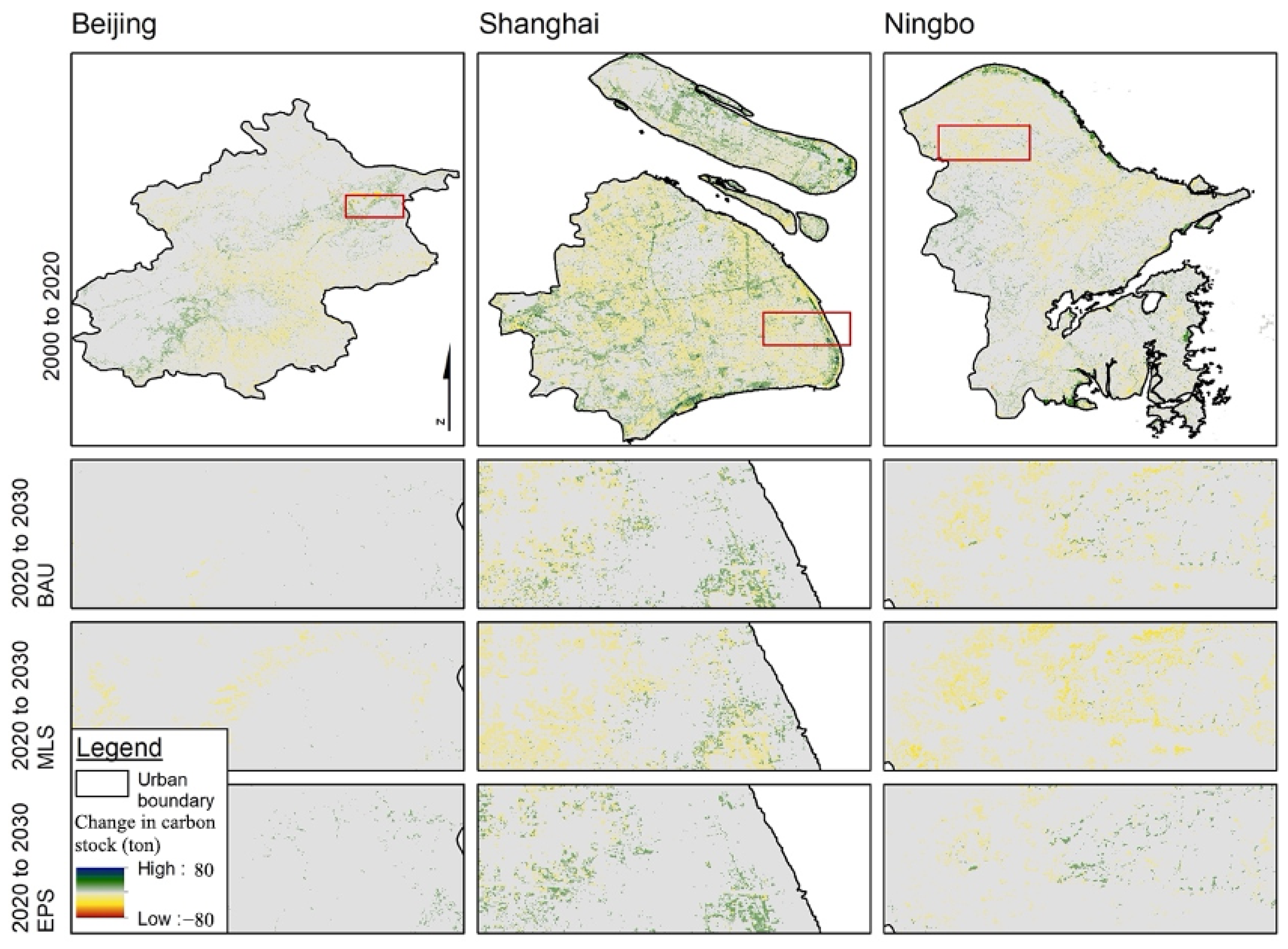
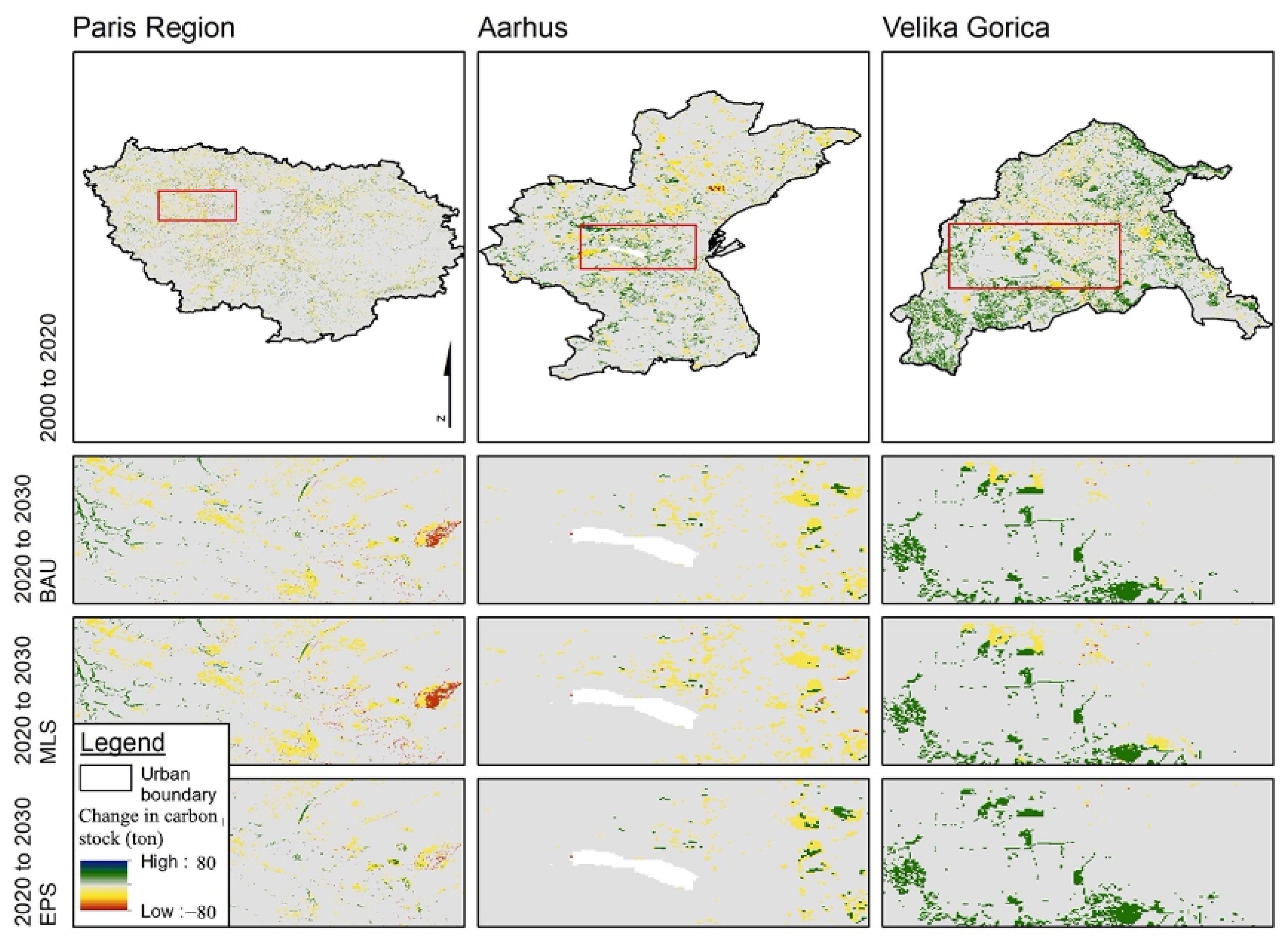
4.2.2. Dynamics in Carbon Stock
Figure 7 and
Figure A4 show the distribution of carbon stock changes from 2000 to 2020 and 2020 to 2030 under different scenarios. Between 2000 and 2020, some areas of the long-term built-up areas in Beijing and Shanghai have greater carbon stocks, with increases in the southwestern and southeastern parts of Beijing and increases in Shanghai mainly in the outer ring green belt and Chongming Island. For Ningbo, the carbon stock shows a decreasing trend between 2000 and 2020. From 2020 to 2030 under various scenarios, there is a significant increase in carbon stock in the EPS scenario relative to the BAU and MLS. As for the three cities in Europe, from 2000 to 2020, carbon stock shows a stable trend in the Paris region, while in Aarhus, there is a strong increasing trend in carbon stock in the south of the city. In Velika Gorica, the carbon increase was significant throughout the region, especially in the forest area.
Figure A5 shows the changes of carbon stock in different urban development phases. Among the six cities, in 2020, Beijing has the largest carbon stock with 210.7 Mt, followed by the Paris region with 140 Mt. There is a slight increase in the long-term built-up carbon stock in Shanghai between 2010 and 2020, from 11.9 Mt to 12.4 Mt. Under different development scenarios, the most carbon stock is found in the EPS scenario. For example, in China, the total carbon stocks of the three cities in the EPS scenario are 7.1 Mt and 14.3 Mt more than those in the BAU and MLS scenarios, respectively. The Chinese cities generally show much more carbon in the newly built up areas compared with old built-up areas, when compared with European cities. Shanghai in particular shows a large proportion in newly built-up compared with the total study area (
Figure A5).
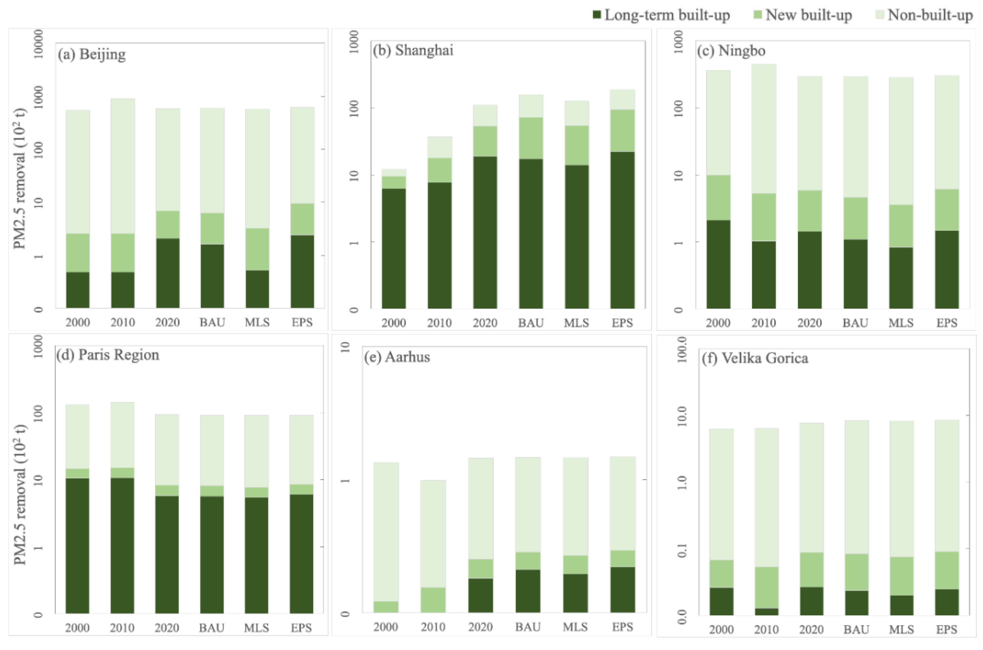
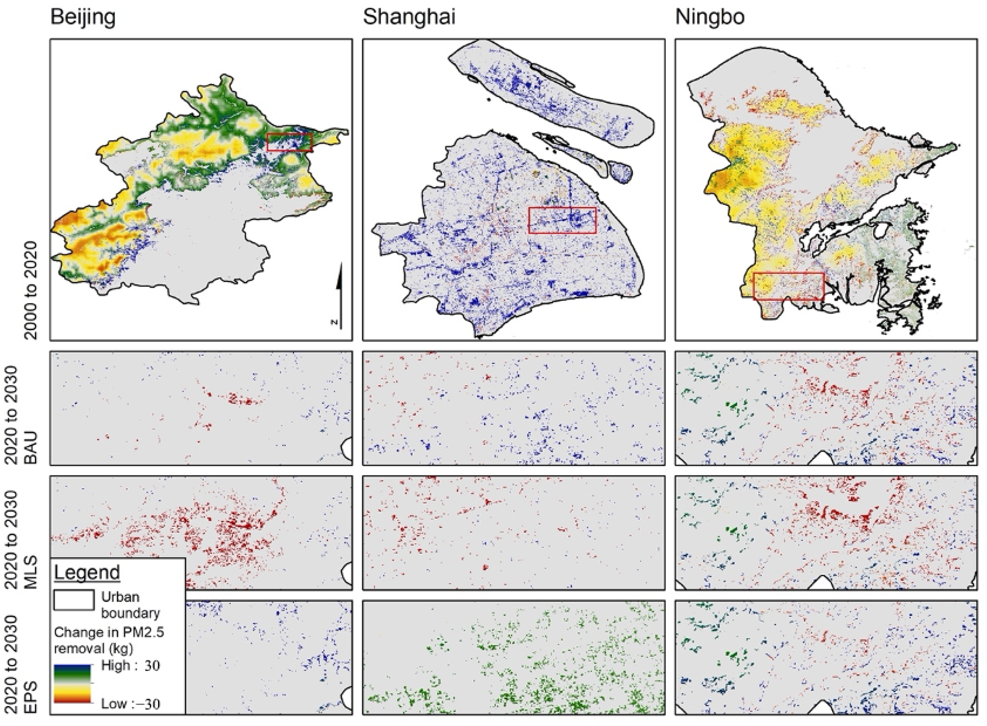
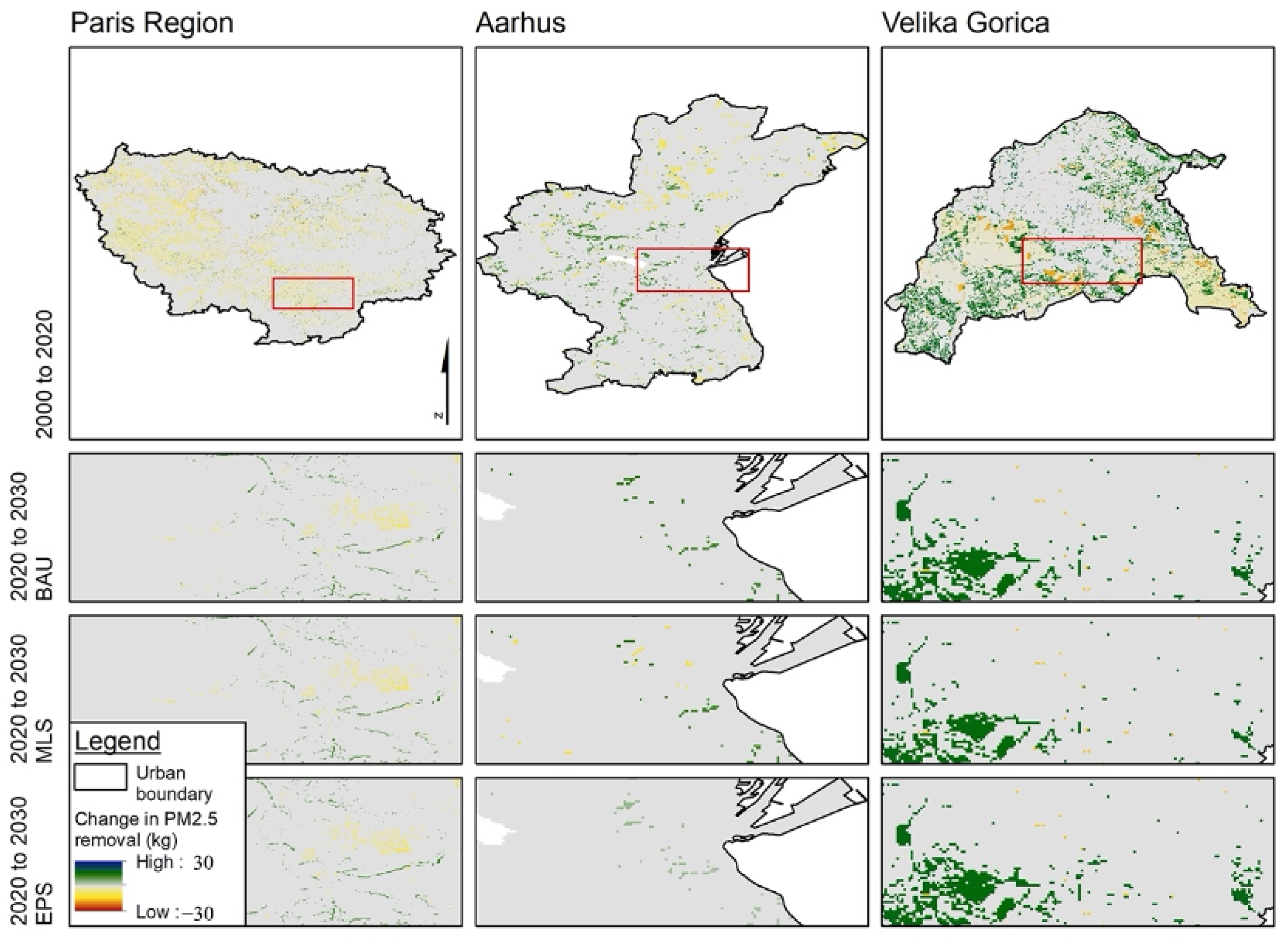
4.2.3. Dynamics in PM2.5 Removal
Figure 8 and
Figure A6 show the dynamics of PM
2.5 removal under different development scenarios from 2000 to 2020 and from 2020 to 2030. Between 2000 and 2020, both Shanghai in China and Velika Gorica in Europe exhibit large increases in PM
2.5 removal. The results for regions at different phases (
Figure A7) of urban development show that Beijing has the highest PM
2.5 removal among the six cities. The level of PM
2.5 removal in Shanghai substantially increased from 2000 to 2020 and continued to increase slightly in 2030, especially under EPS. For Ningbo, the amount of PM
2.5 removal increased from 2000 to 2010 but then decreased in 2020. PM
2.5 removal in the Paris region experienced an increase up to 2010 and then a decrease in 2020, with insignificant differences in PM
2.5 removal among the three future scenarios. For Aarhus and Velika Gorica, their PM
2.5 removals are much lower compared with the other cities, with insignificant changes in the values of PM
2.5 removals for Aarhus in each year. Detailed information about the dynamics of GI and ES in different urban development stages and different years are available in the supporting materials (
Table A4,
Table A5,
Table A6 and
Table A7).
4.3. Sensitivity of GI and ES to Land-Cover Changes
Table 2 shows the SI of various indicators related to land-cover changes. Overall, most of the SIs for the four different indicators are less than 0, indicating that land-cover changes in the six cities have a negative impact on the coverage and connectivity of GI, as well as on the amount of carbon sequestration and air pollution removal. Based on observations from 2000 to 2020, land-cover change showed a positive effect on carbon stock and PM
2.5 removal from 2000 to 2010 in Beijing, while land cover in Shanghai continued to positively affect carbon stock and PM
2.5 removal from 2000 to 2020. In Ningbo, land-cover change had a positive effect on PM
2.5 removal only from 2000 to 2010. For the three European cities, land-cover change had a small positive effect on carbon stock and PM
2.5 removal between 2000 and 2020, while in Aarhus, the land cover had a positive effect on carbon stock and PM
2.5 removal between 2010 and 2020, where SIcarbon was 0.02, and SIpm
2.5 was 4.16. In Velika Gorica, there was a continuous positive effect of land cover on both carbon stock and PM
2.5 removal between 2000 and 2020.
Under the three scenarios in 2030, land-cover change had a negative impact on all four indicators to varying degrees. The impact of land-cover change on ES was most pronounced under MLS, with an average SI of −1.95. It is worth noting that in the Paris region, land-cover change positively affects both carbon stock and PM2.5 removal under EPS.
4.4. Equity of GI Distribution
In order to better understand changes in the distribution of GI in areas that rarely experience urban expansion, in
Table 3, the GINI coefficients are shown as a function of the GIF distribution of long-term built-up areas on a 1 km × 1 km grid between 2000 and 2030. According to the results, GINI coefficients of GIF distributions from 2010 to 2020 decreased for Beijing and Shanghai, indicating a greater equity of GIF in the long-term built-up areas of the region. By contrast, for Ningbo, the GINI coefficients increased from 2000 to 2020, indicating an increasing inequity of GIF distributions. Among the three European cities, the GINI coefficients of the GIF distribution in the long-term built-up area vary less, and Velika Gorica has the smallest GINI coefficient of the GIF distribution in the stable built-up area, with a GINI value of 0.1 in 2020 and a GINI value of 0.24 in the EPS scenario in 2030. The GINI coefficient values increase the least in the EPS scenario in 2030, indicating that the EPS scenario is also a guarantee of the equity of the GIF distribution. In all cases, the GINI coefficients are greatest (i.e., greatest inequity) in the MLS scenario.
5. Discussion
Urban development stages and policies directly affect the quantity and distribution pattern of GI, which in turn affects the equity of distribution of ES. This study enables a robust multi-context prediction of future land cover in cities and provides an assessment of past and future GI and ES functions.
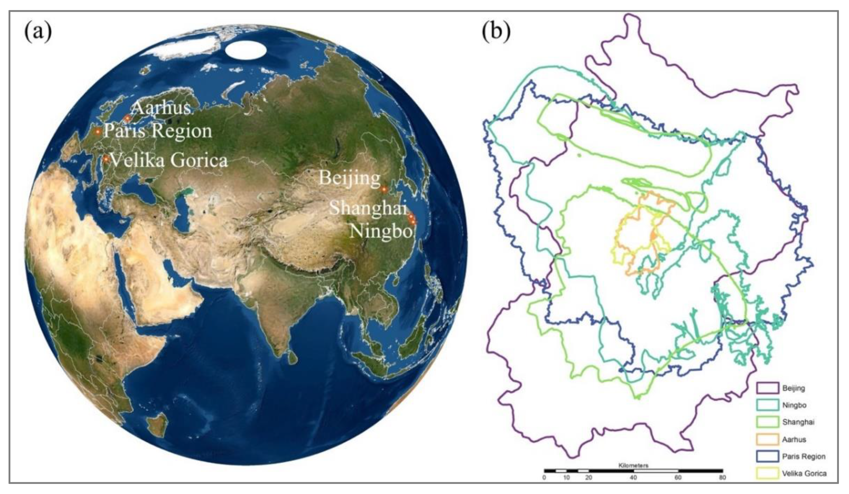
The selection of six contrasting cities in China and Europe exemplifies the evolution of ES for fairly typical sizes of towns, cities, and megacities to illustrate impacts of ongoing urbanization processes. On the one hand, due to the difference of urbanization process and stage between China and Europe, the dynamic changes in land cover and ES showed substantial differences for similar time points. Specifically, Europe is a highly urbanized continent, while China is progressing rapidly towards an urbanized country over the last decades. Therefore, urban expansion in the three Chinese cities caused significant damage to the coverage and connectivity of urban GI and the ES it provides [
53]. In contrast, national land cover and ES in Europe have shown more moderate changes.
Specifically, the multi-scenario analysis provides urban planners and policy makers with more dimensions of reference, which may guide urban planning policies by demonstrating the characteristics of ES distribution and their impacts under different scenarios. In addition to the extensive research on the spatial and temporal dynamics of ES, the resulting environmental equity is also receiving increasing attention because it is essential for equitable urban policy making [
54]. Recent studies show that the loss of ES equity can affect not only ethnic groups of people differently [
55], it is also essential in order to attain the social inclusion that is part of SDG 11 [
56]. Quantifying ES distribution patterns helps increase the understanding of its contribution to environmental equity and use it as an important reference for reallocating ecological resources.
Moreover, the multi-regional analysis distinguishes between the impacts of urbanization on ES at different stages of urban development, i.e., long-term, new, and non-built-up areas [
14,
53], which is useful to increase the understanding of how ES are affected by different urbanization intensities and dynamics. The focus on long-term built-up areas also provides insight into the status and recovery of ES in urban centers that are not subject to urban sprawl or in the post-urbanization phase, and, as revealed in China, that there is potential to retrospectively improve GI provision at large scale within existing urban areas. For example, the values and distributional balance of GI and ES in long-term built-up areas in Beijing and Shanghai, China, improved between 2010 and 2020, indicating a return to green in these cities, which is a direct outcome of government policies [
1].
In particular, in the early stages of urban development, such as from 2000 to 2010, most regions of China experienced rapid urbanization and urban sprawl, and many blue-green elements were directly replaced by built-up areas, resulting in a direct loss of GI coverage and ES. During the latter stages of development, GI and ES have improved in long-term built-up areas with a higher demand for ES, as seen in Beijing and Shanghai from 2010 to 2020. As compared to the three Chinese cities, the European cities have experienced longer-term development and slower urban expansion in the past decades, so the EPS scenario is more likely to maintain and optimize ES in Chinese cities in the future.
The study examined both GI and ES in order to explore the comprehensive effects of urbanization and policies on urban ecosystems. Specifically, a high GIF, for instance, contributes to an inclusive, resilient, and sustainable urban development [
57]. In addition to regulating urban microclimate and reducing urban heat islands, adequate green space also prevents surface runoff and floods as well as provides residents with habitat, recreation, and cultural opportunities [
58,
59,
60]. Furthermore, GIC reflects the loss of natural habitat mentioned in SDG 15.5 and its consequences for biodiversity [
61,
62]. This is because natural vegetation corridors provide adequate connectivity, allowing species to move freely and contributing to biodiversity preservation, while low connectivity isolates species and threatens biodiversity [
63]. The benefit of carbon stock as one of the main ES is that the absorbed carbon dioxide from the air in urban vegetation is bound to organic carbon through photosynthesis and ultimately stored. As PM
2.5 does great harm to the health of urban residents, we analyzed this indicator as, to a certain extent, it is captured and removed through the atmospheric process of dry deposition to vegetation surfaces.
For the uncertainty of the study, because of the high heterogeneity of land cover in urban centers, there are inevitable errors in both the mapping and simulation of land cover and which further lead to uncertainty in ES assessment. These uncertainties in ES assessment have also been explored extensively in previous studies [
64]. Different spatial resolutions and time lags between historical and future parameters, available for land-cover simulations, may lead to uncertainties in the results. In future studies, the accuracy of land-cover simulations can be effectively improved by using more high-resolution inputs and more homogeneously stored spatial information, such as new road plans and established future protected areas. Furthermore, interpreting results of the ecosystem service model outputs is not straightforward, since the models include other components. For example, in the estimation of PM
2.5 removal, the model used in this study is sensitive to the initial concentration of PM
2.5 as well as the removal capacity of trees [
65]. Therefore, interpreting the final results requires knowledge about how other aspects (e.g., air pollution levels) are changing at the same time. When estimating carbon stock, the carbon density parameters were obtained from the literature but could be improved with more detailed data collected for each city.
6. Conclusions
Urbanization processing and policies can directly affect urban land cover patterns and further influence ES. In this study, six cities of different sizes from China and Europe were selected as case areas, and a framework for an integrated assessment of urban ecosystem service dynamics under different development scenarios (BAU, MLS, and EPS) in the past and future was proposed. Additionally, this study focuses on the dynamics and changes in the variability and equity of GI and ES among different cities (Chinese and European cities) and within cities at different stages of development, as well as quantifying the sensitivity between changes in each indicator with respect to land-cover change. The main conclusions of the study are as follows: (1) The use of multi-source remote sensing data and the CLUE-S model can simulate future urban land cover distribution patterns under different development scenarios, and the simulation accuracy performs well in cities of different scales. (2) Urbanization levels in China and Europe are still at very different stages of development, not only in terms of the intensity of land-cover changes but also in terms of the characteristics of the changes in GI and ES. (3) Long-term built-up areas can be an important indicator of urban regeneration and ecosystem restoration; e.g., Beijing and Shanghai in China have seen significant improvements in both green space coverage and equity and ES in long-term built-up areas over the last decade. (4) In the future, the expansion of built-up areas will remain the main trend, and the loss of green space and arable land will be greatly reduced in EPS scenarios compared to BAU and MLS, while the green space cover in stable built-up areas is more fragile and should be a priority area for protection. The results obtained from this study can be used as an important reference for urban planners and policy makers at a later stage.


