Spatial Modelling of Vineyard Erosion in the Neszmély Wine Region, Hungary Using Proximal Sensing

Abstract

Intense soil erosion in the northern part of the Gerecse Hills, Hungary, is causing significant damage to vineyards in the area. Three vineyards in the Neszmély Wine Region were investigated to quantify the amount of eroded soils. The method was based on monitoring vineyards for one-year between July 2019 and June 2020. Every season, a set of photographs of the vineyards were taken from an unmanned aerial vehicle. The images were processed in a photogrammetric workflow to produce high-resolution digital terrain models (DTMs) and orthophotos, which were used to estimate the soil loss using the Universal Soil Loss Equation (USLE) model. Particular attention was paid to the effect of seasonal variation in vegetation cover and rainfall, and the erosion control effect of the inter-row grassing already applied in the vineyards was also modelled. The results confirm and quantify the extent to which intense summer rainfall has a more significant effect on erosion compared to autumn or winter rainfall.

1. Introduction

Soil is one of the essential components of land and therefore agriculture. Degradation occurs when soil formation can no longer keep up with the rate of soil erosion. The natural process of soil degradation is strongly influenced by human activity in agricultural areas. Soil degradation is a complex process, which can cause loss of land or decrease soil fertility; therefore, soil degradation places plantations at risk of becoming unsustainable. These consequences increase with the intensification of climate change. The way to control erosion is to reduce the impact of triggering factors and to influence the modifying factors to reduce the rate of soil degradation, among other methods which are as follows [1,2,3]:

• The use of appropriate slope adjustment techniques, i.e., slope grading or terracing;
• Changing the type of cultivation;
• Slab formation perpendicular to the slope direction;
• The use of appropriate tillage practices;
• The use of soil protection planting [4].

The study of soil erosion is still an important research topic today, not only internationally but also at the national level [5,6,7].

Vineyards are among the areas that are most exposed to erosion. The influencing factors of this exposure are hilly and mountainous topographies with slopes, lack of vegetation, the use of heavy machinery, soil properties and climate [8]. In order to maintain the sustainable management of these areas it is essential to control soil erosion. There exist many practices which can be used to reduce the effect of erosion such as terracing, diversion ditches, buffer strips, inter-row soil management and mulch applied in row middles [9,10]. In Hungary, the use of inter-row sodding is prevalent [11], which can be permanent or periodical. Permanent sodding can be applied to all rows or every second row, and can be either sown or left with natural weed flora.

More extensive spatial estimations of soil erosion rates are determined by using satellite remote sensing data and meteorological measurements, as well as geospatial methods based on knowledge of the soil properties of the area [6]. These methods have also been successfully applied to near-surface remote sensing data, which can be used to produce high-resolution (cm/pixel level) models [12,13]. The latter method can be applied to smaller but also contiguous areas. Fernandez et al. [14] studied the formation of erosion furrows in olive groves in Spain, and Pijl et al. [12] applied this method to soil erosion estimation in vineyards in northern Italy. A similar model was developed in agricultural fields in Canada [15]. In Nepal, terraced cultivation erosion studies used near-surface remote sensing data [16]. In the previously mentioned studies, various erosion models were applied at a sub-meter resolution, e.g., USLE, RUSLE (Revised Universal Soil Loss Equation) and SIMWE (SIMulated Water Erosion).

A number of previous studies focused on surface evolution in the area of the Gerecse Hills, which show that both soil erosion and landslides are significant land-forming factors in the present, e.g., [17,18,19,20]. The study area belongs to one of the well-known wine regions of Hungary, the Neszmély wine region. A major vineyard and winery of this wine region is the Hilltop Neszmély Ltd., Meleges-hegy, Hungary. In this area, several plantations of the company are threatened by soil erosion. The aim of this study was, by conducting short- and medium-term monitoring of vineyards at risk of high erosion, to produce seasonal, high resolution (10 cm/pixel) soil loss maps of the study areas. These were used to define critical zones within vineyards at high risk of erosion, and to estimate the soil loss and its dynamics of change during the year in each area.

2. Materials and Methods

2.1. The Neszmély Wine Region and the Study Sites

The territory of the Neszmély wine region is about 1400 ha in the northern part of the Transdanubia, Hungary. The center of the wine region can be found in the western and northern slopes of the Gerecse Hills.

The wine-growing area is characterised by brown forest soils formed on loess, but also by dolomite and limestone, as well as brown forest soils formed on sandstone and marl [21].

The Neszmély wine region has a unique microclimate influenced by the hilly nature of the area and by the warm currents arriving from the Little Hungarian Plain. It is also influenced by the Danube which provides a moderately wet and cool climate. On the north-facing slopes, the river reflects back the sun’s rays and creates a favourable climate for the viticulture. The number of sunshine hours is 2000–2050 and the yearly precipitation is 550–650 mm [22].

The soil types and the climate of the area make the wines produced here highly acidic and therefore suitable for long-distance transport, meaning large quantities are shipped abroad. White grapes are the main grape varieties grown in the area, such as Sauvignon Blanc, Irsai Olivér, Ezerjó and Chardonnay. The Neszmély wine region can be divided into the following two districts: the Ászar and the Neszmély district.

The study sites are located in the Neszmély district, near Dunaszentmiklós, in the area of the Hilltop winery (Figure 1). The first field observation took place in July 2019. The staff of the viticulture were also interested in the research topic and helped us to select the sample areas. They informed us about areas of concern for the high and rapid rate of soil degradation. We compared this information with the results of previous erosion and landslide studies [19,20]. Finally, soil erosion was estimated for a total of 63.4 ha in three study sites, where high levels of soil degradation were observed based on the medium-scale models and local experiences.

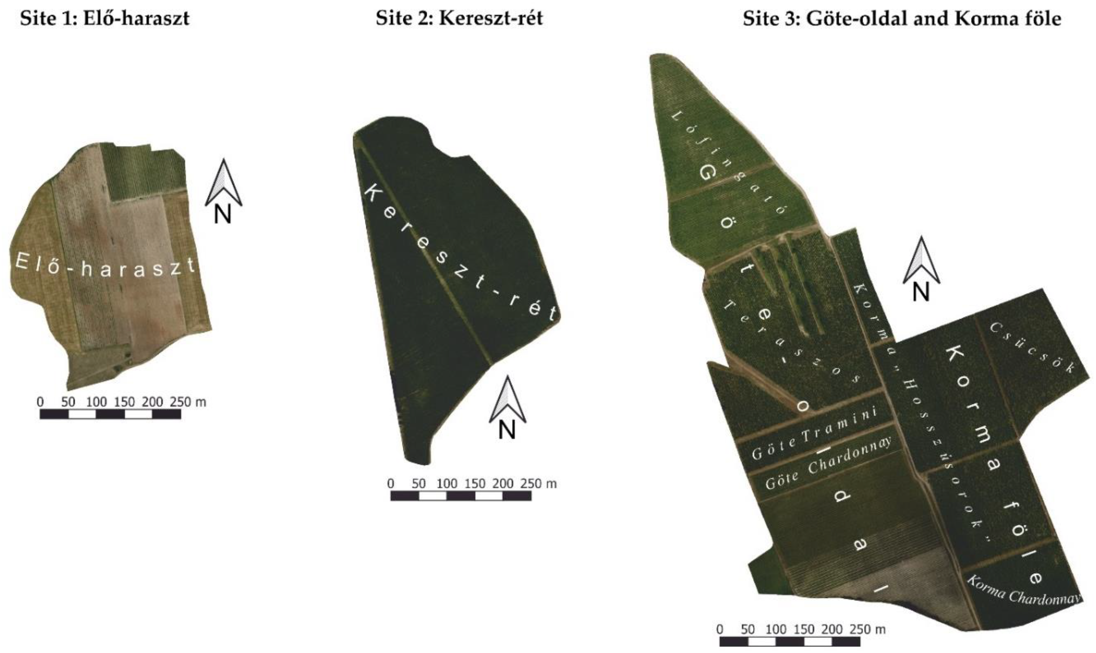
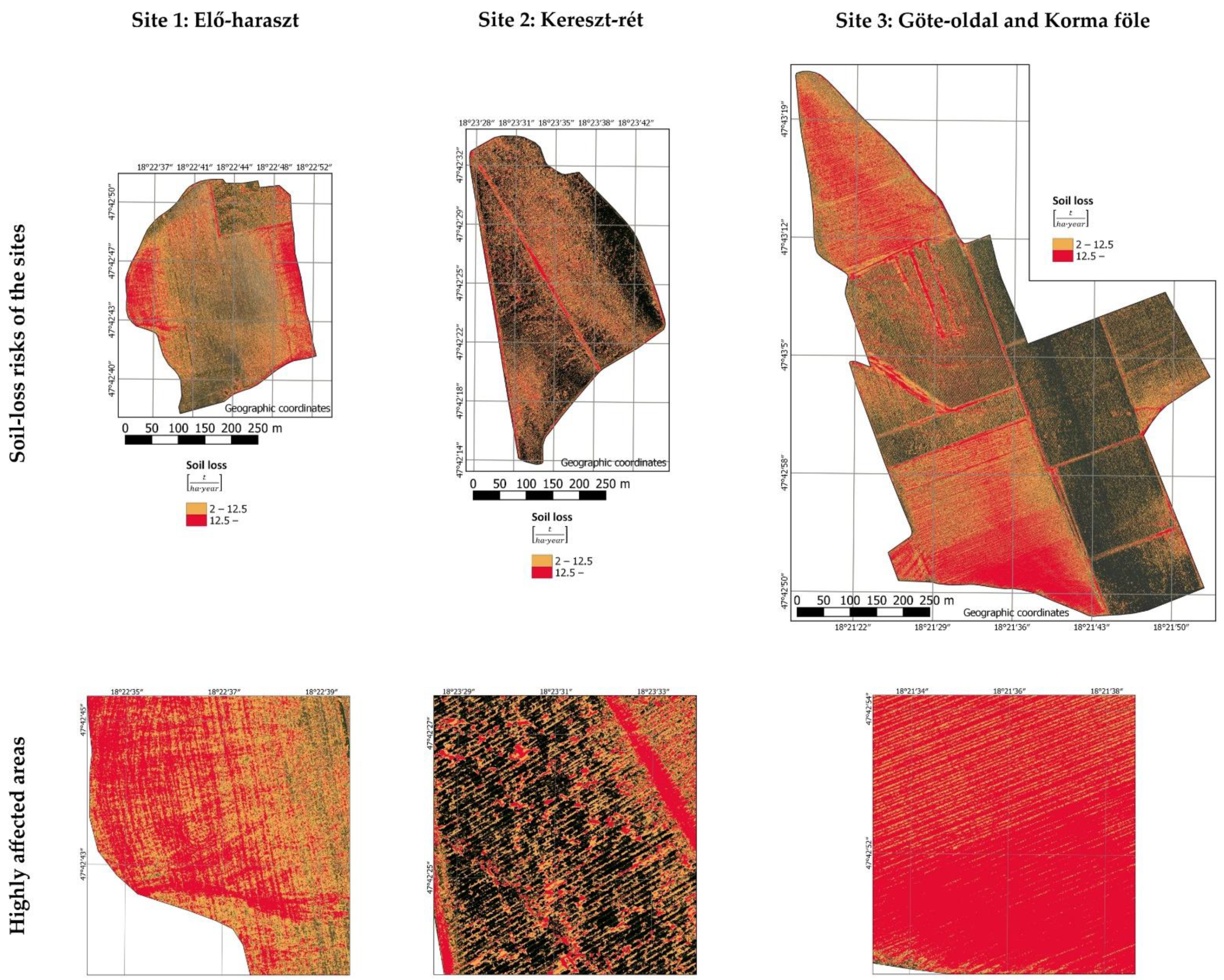
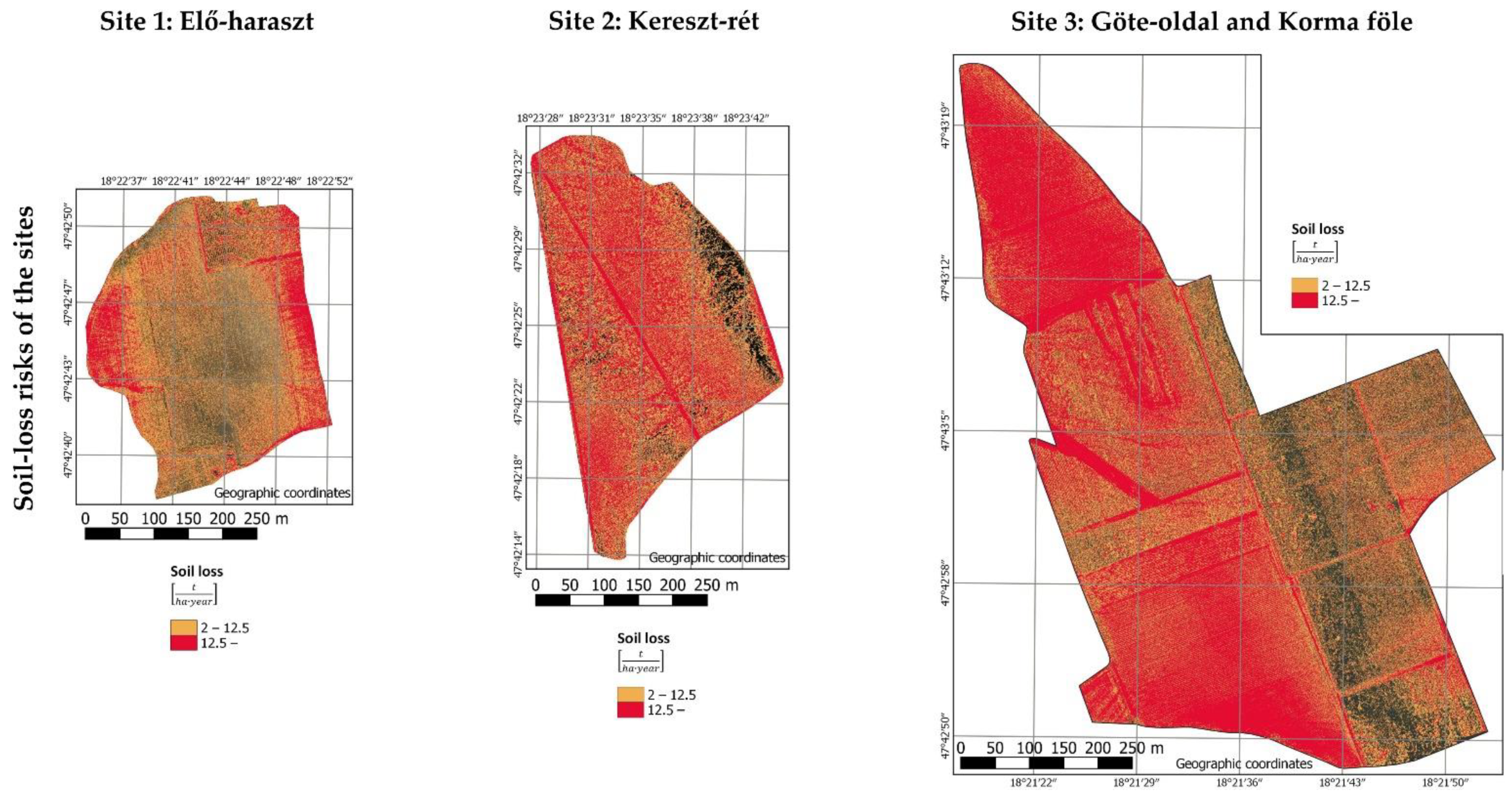
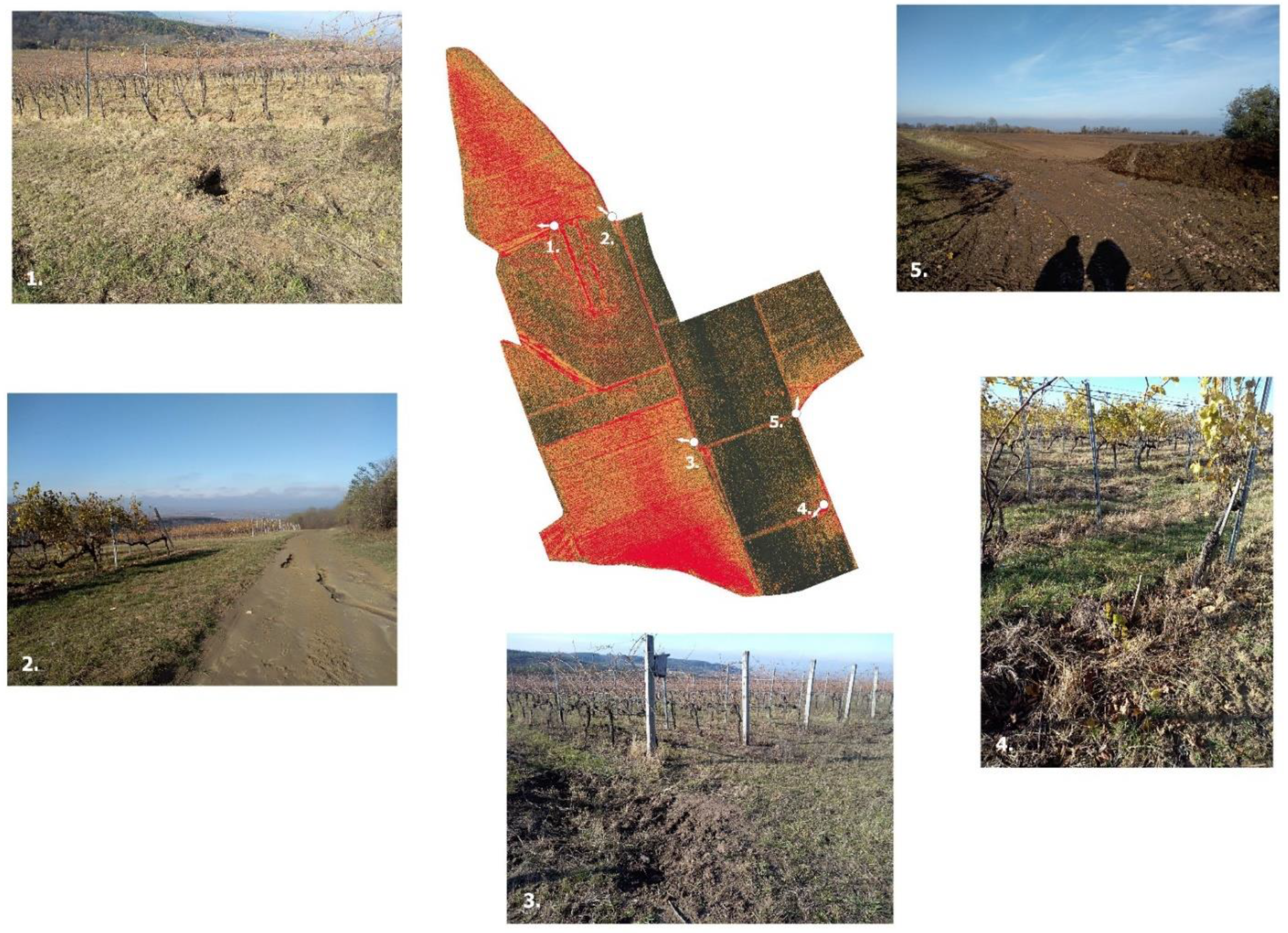
The names of the areas were derived from the names of the vineyards and the parcel names used by the winery, which were as follows (Figure 2): site 1: Elő-haraszt, site 2: Kereszt-rét, site 3: Göte-oldal, and Korma föle. The serial numbers below refer to the territories mentioned before.

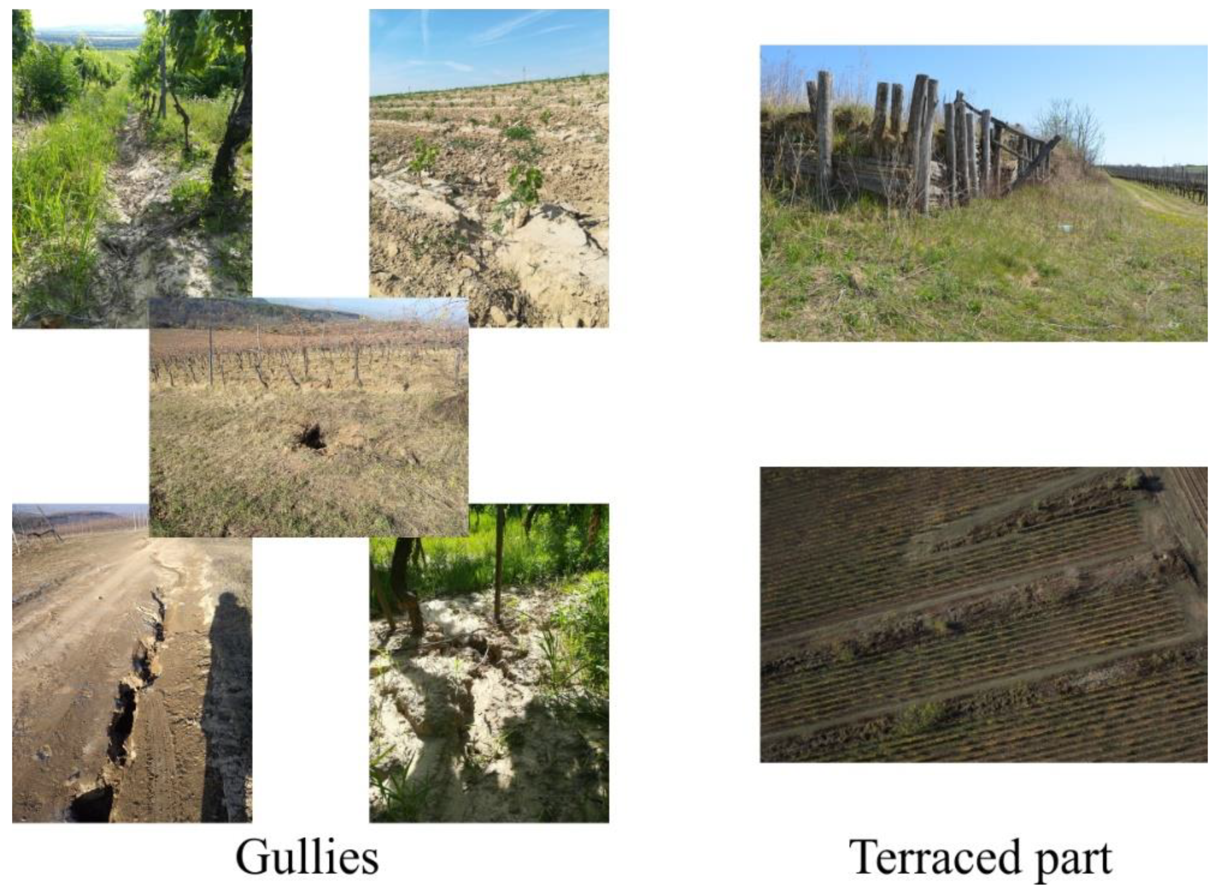
In site 1, the focus was on the part of the Elő-haraszt where young vines were planted in 2018. Therefore, in this field, the vines were still small, so it was possible to observe the uncovered soil. The eastern and western parts of site 1 were arable land. Site 2 was crossed by a large gully and the rows of vines were grassed between. Site 3 had a varied soil surface. Some parcels were grassed among the rows, while others were not. Several gullies were observed in this field (Figure 3, ‘Gullies’). In a particularly endangered part of the area, there were three terraces where the vines could not be cultivated by machines for fear of landslides occurring under the machinery (Figure 3, ‘Terraced part’). The vine deficit was greatest in the “Teraszos” parcel. In the “Csücsök” parcel (Figure 2), the vines were taken out in autumn 2019 and replanted in spring 2020. The winery performs several measures to slow down soil erosion. One of the measures is the permanent grassing between the rows of vines since 2017. According to the operators’ observations, soil erosion has visibly decreased since then.

2.2. The Aerial Surveys

The project was based on a year-long series of observations, with drone surveys of the study sites in each season. The dates, weather conditions and outcomes of the field surveys are presented in

Table 1. Field measurement data and photographs of the study sites.

	Date	Weather
Field trip	5 July 2019	warm, sunny
Summer survey	24 July 2019	warm, sunny
Autumn survey	14 November 2019	Warm, similar to spring, sunny
Winter survey	19 February 2020	cold, slightly windy, sunny
Spring survey	10 April 2020	sunny, windy

. Three different types of UAVs were used during the surveys. The use of different UAV devices was not a problem during processing, as all cameras had a similar type of sensor and a standardised lower spatial resolution (10 cm) was used to determine soil erosion.

The data of the first two surveys were recorded using a Ricoh GR II compact camera mounted on a home-developed drone. The camera has a CMOS (Complementary Metal Oxide Semiconductor) sensor, an effective resolution of 16.2 MP and pixel resolution of 4928 × 3264. A proprietary 28 mm lens was used that provides a high-resolution image free of distortion and chromatic aberration right up to the edge of the frame. The spatial resolution of images taken with this sensor was originally in the range of 2.62–3.32 cm. The UAV was also equipped with an RTK (Real-Time Kinetic) GPS receiver, which provided high accuracy positioning. Before the flights started, a base station was installed at the winery site to provide correction data. During processing, all other measurements were adjusted to the first survey, i.e., the summer 2019 measurements.

During the winter survey, a DJI Phantom 4 Pro drone was used to record the images. The built-in camera had a 1” CMOS sensor with an effective resolution of 20 MP and pixel resolution of 5472 × 3648, which improved the signal-to-noise ratio and the quality of images taken in low light conditions. This device also had a GPS receiver, which assigned the current coordinates to each photo, but it is not suitable for high-precision positioning. Its inaccuracy was mainly observed in the altitude data, but this did not affect the analyzability of the images.

For the spring survey, a new UAV with a Fujifilm X-T20 MILC (Mirrorless Camera) (Fujifilm Corporation, Tokyo, Japan) camera was used. This device also had a CMOS sensor. The effective resolution of the camera was 24MP and the pixel resolution was 6000 × 4000. For the latter two devices, the camera was mounted on a triaxial stabilizer (gimbal) and the spatial resolution of the images were between 3.00 and 3.29 cm. As the optics of each camera had a wide angle of view, the UAVs flew 120 m above the terrain and took pictures of the surface every 4–5 s. In each case, the flight plan was generated using autonomous flight planning software (Mission Planner ver. 1.3.77 (ArduPilot Development Team, Pix4D Capture), which allowed for the live tracking of the UAV with flight information (speed, altitude, etc.).

2.3. Data Processing

The drone images were used to create an orthophoto and a surface and terrain model using photogrammetric methods (MetaShape [23] and CloudCompare [24] programs). The processing of the summer survey differed slightly from the others. In this case, the coordinates of the images were obtained from the RTK GPS mounted on the drone.

The coordinates were used in the process (i) to place the photos in their real spatial position, (ii) to perform an overlay analysis of the images and (iii) to produce a spatial point cloud model based on the SFM (Structure from Motion) principle. The dense point cloud categorization by height is used to select ground points, i.e., to filter vegetation cover, and thus to produce the high resolution digital terrain model (DTM) and its geometry for the orthophoto. A shape file was consistently used to delineate the study sites for each seasonal exposure.

On subsequent occasions, the individual images were not always accompanied by appropriate GPS data, so Ground Control Points (GCPs) were defined in the summer images. These data were stored in a text file (txt). The points were used for the spatial alignment of the autumn, winter and spring images by marking their locations on the images. In this way, the spatial arrangement of the images was adapted to the summer measurement. After performing spatial fitting, the point cloud of the surface models was created, and then the processing procedure was the same as mentioned before. The resulting terrain models and orthophotos were exported at a resolution of 10 cm/pixel.

The resulting terrain models were used to estimate the soil degradation and to determine the morphometric factor and tillage method. DTM processing and spatial data management were performed in the QGIS software environment [25]. The orthophotos were used to determine the vegetation cover classes.

2.4. Erosion Estimation Using the Universal Soil Loss Equation

The main objective was to produce high-resolution soil loss maps for vineyards at a high risk of erosion, which would allow us to measure the variation of soil erosion rates between seasons. The maps were produced as a series of raster-based spatial data analyses, with cells as the basis for the calculations of unit areas.

To determine the soil loss per unit area, the Universal Soil Loss Equation (USLE) was used. Each factor in the equation expresses how the climate, soil, surface morphology, land cover or cultivation method affects the rate of soil loss. The equation can be used to calculate an estimate of the average soil loss over a given area per year (or other specified period). The equation was developed in the United States in the 1940s [26]. Initially, the method used Anglo-Saxon units of measurement, and in 1981 the SI (Systeme International d’Unites) version of the equation was developed [27]. Since then, the equation and its improved versions have been widely used to estimate soil degradation [28,29,30,31]. The equation contains six spatial variables, which are multiplied by the soil erosion rate per unit of time (in the formula, per year):

A = R∙K∙L∙S∙C∙P

(1)

$$\mathrm{A}=\mathrm{average} \mathrm{annual} \mathrm{soil} \mathrm{loss} \left[\frac{\mathrm{t}}{\mathrm{ha}·\mathrm{year}}\right]$$

(2)

$$\mathrm{R}=\mathrm{rainfall} \mathrm{and} \mathrm{runoff} \mathrm{erosivity} \mathrm{factor} \left[\frac{\mathrm{MJ}·\mathrm{mm}}{\mathrm{ha}·\mathrm{h}·\mathrm{year}}\right]$$

(3)

$$\mathrm{K}=\mathrm{soil} \mathrm{erodibility} \mathrm{factor} \left[\frac{\mathrm{t}·\mathrm{ha}·\mathrm{h}}{\mathrm{ha}·\mathrm{MJ}·\mathrm{mm}}\right]$$

(4)

L = slope length factor (dimensionless)

(5)

S = slope steepness factor (dimensionless)

(6)

C = crop cover factor (dimensionless)

(7)

P = factor for the type of tillage applied (dimensionless)

(8)

In this study, the value of “A” refers to each season, so the precipitation data were considered for summer (June–August), autumn (September–November), winter (December–February) and spring (March–May) time intervals.

2.4.1. R Factor

Soil degradation depends on the intensity of rainfall and the size of raindrops. The R-factor expresses the kinetic energy of precipitation, which includes the erosion index of each rainfall event and information on the amount and rate of runoff. The R factor is given in $\left[\frac{\mathrm{MJ}·\mathrm{mm}}{\mathrm{ha}·\mathrm{h}}\right]$ [26].

The R factor was calculated using the equation converted to SI units. For each rainfall event, the kinetic energy was determined using the following Formula [32]:

$$e_c=0.119+0.0873·log i$$

(9)

$e_c:$ is the kinetic energy for each rain segment $\left(\mathrm{MJ}·{\mathrm{h}}^{-1}·{\mathrm{mm}}^{-1}\right)$

$i:$ is the rainfall intensity of each segment $\left(\mathrm{mm}·{\mathrm{h}}^{-1}\right)$

We determined the total kinetic energy in each rain segment as follows $\left(E_{s , }in \mathrm{MJ}·{\mathrm{ha}}^{-1}\right)$:

$$E_s=e_c·p$$

(10)

The total kinetic energy of the rain $\left(E_{t , } in \mathrm{MJ}·{\mathrm{ha}}^{-1}\right)$:

$$E_t={\displaystyle \sum }{E}_s$$

(11)

Multiplying the total kinetic energy of the rain by the greatest intensity for 30 min we gained the erosivity index $\left(E{I}_{30 , } in \mathrm{MJ}·\mathrm{mm}·{\mathrm{ha}}^{-1}·{\mathrm{h}}^{-1}\right)$ of each rain event as follows:

$$E{I}_{30}=E_t·I_{30}$$

(12)

$I_{30}:$ is the greatest maximum intensity in 30 min $\left(\mathrm{mm}·{\mathrm{h}}^{-1}\right)$

Precipitation data for the calculation of the R factor were provided by the National Meteorological Service of Hungary (OMSZ). Hourly data were available from two permanent monitoring stations closest to the study area, which were (1) Gerecse-tető and (2) Tata, Új út. Therefore, we could only make an estimate of the greatest 30 min intensity by taking half of the amount of the hourly measured precipitation. During the monitoring year, the Gerecse-tető station recorded 581.6 mm of precipitation, while the Tata, Új út station recorded 471.4 mm.

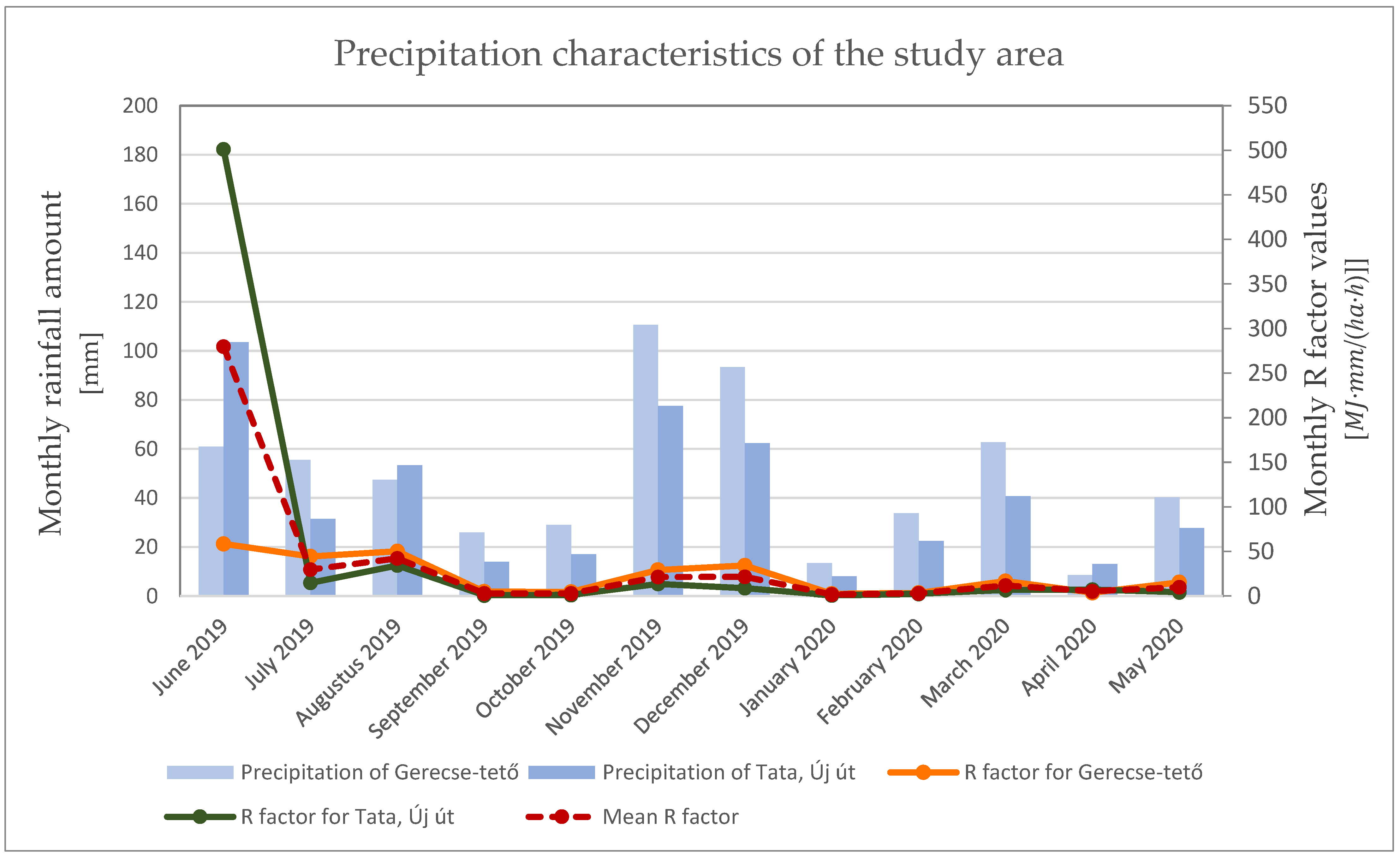
To obtain the erosion equation, it was necessary to calculate the monthly cumulative amount of precipitation and the value of the R factor (Figure 4). In the available, data a prolonged period of light rainfall and sudden bursts of heavy rainfall with short duration was observed. The erosion was estimated by summing the R factor values by season.

Three months with exceptionally high rainfall were June, November and December. The monthly R values show that rainfall had a much greater impact on soil erosion in June than in November or December. This is because of the prolonged period of light rainfall (with 0.13 mm/h mean intensity [sd: 0.61 mm/h]) in November and December, while the evening of 22 June saw a sudden heavy rainfall event (with 53.6 mm/h intensity).

The seasonal R-factor was obtained by summing the erosion indices within a season, i.e., over three months, and used in the estimation of soil erosion (

Table 2. Seasonal R values.

Season	$\mathbf{R} \mathbf{Factor} \left[\frac{\mathrm{M}\mathrm{J}\mathrm{·}\mathrm{m}\mathrm{m}}{\mathrm{h}\mathrm{a}\mathrm{·}\mathrm{h}\mathrm{·}\mathrm{s}\mathrm{e}\mathrm{a}\mathrm{s}\mathrm{o}\mathrm{n}}\right]$
Summer	351.59
Autumn	27.19
Winter	26.22
Spring	27.02

).

2.4.2. K Factor

The K-factor indicates the soil erosion susceptibility, which is influenced by several soil properties, such as soil structure, soil particle composition, soil permeability, organic matter and clay mineral content [26]. These primary soil properties can be used to estimate the value of K, for which a one-hectare resolution map dataset edited by Pásztor and colleagues [33] was used in the present study. The K factor values for the study sites fell within the intervals indicated in

Table 3. K-factor values for each site.

Site	$\mathbf{K} \mathbf{Factor} \mathbf{Values} \left[\frac{\mathrm{t}\mathrm{·}\mathrm{h}\mathrm{a}\mathrm{·}\mathrm{h}}{\mathrm{h}\mathrm{a}\mathrm{·}\mathrm{M}\mathrm{J}\mathrm{·}\mathrm{m}\mathrm{m}}\right]$
1. Elő-haraszt	0.027–0.029
2. Kereszt-rét	0.028–0.030
3. Göte-oldal/Korma föle	0.026–0.030
1. Elő-haraszt	0.027–0.029

.

2.4.3. LS Factor

The morphometric element of the USLE equation is the Slope Length and Steepness factor (LS factor). It is composed of two components whereby L is the slope length and S is the steepness. This factor describes the effect of topography on soil erosion and usually has the greatest influence on soil loss.

The LS factor can be calculated from a digital terrain model using GIS tools based on the unit contributing area (UCA) principle [34]. Values for L and S values were generated using the slope steepness and runoff accumulation per cell derived from the high-resolution DTM obtained from drone images. The L factor was calculated according to the method of Wischmeier–Smith [26]:

$$L={\left(\frac{\lambda }{22.13}\right)}^m$$

(13)

λ = slope length.

(14)

The exponent m in the equation is a value that depends on the percentage of slope [35].

s > 5% → m = 0.5;

(15)

3 < s ≤ 5% → m = 0.4;

(16)

1 < s ≤ 3% → m = 0.3;

(17)

s ≤ 1% → m = 0.2.

(18)

The S factor was also calculated using the Wischmeier–Smith equation [26]:

$$S=65.41·si{n}^2\theta +4.56·sin \theta +0.065$$

(19)

θ = slope angle (in radians).

(20)

For each period, flow accumulation maps and slope angle maps of the sites were created and used to determine the L and S factors. Using the two factors as raster data, the LS maps were produced with cell-by-cell clustering.

The resulting maps highlight the major watercourses and their impact on the extent of soil degradation. Seasonal variations were also observed, mainly due to changes in morphology, precipitation and the impact of agricultural activities in the areas.

2.4.4. C Factor

The C factor shows the extent to which land cover and land use affect the soil erosion. This factor can be highly variable both temporally and spatially since vegetation cover plays a significant role in mitigating soil erosion. C factor and its variation during the year can be calculated with the help of NDVI (Normalized Difference Vegetation Index) [36,37,38]. In this work, we did not have a multispectral/hyperspectral camera to calculate the NDVI value for each season and study site. We wanted to quantify the seasonal change in the vegetation; therefore, we determined the C factor based on the orthophotos of the areas.

Seasonal orthophotos from the processing of drone images were used to generate the C factors of study sites. Supervised classification, performed in the Semi-automatic Classification module of QGIS [39], was used to separate the different type of coverages in each season and study site. The three main categories which we wanted to identify were vines, grassland and bare soil. Firstly, we assigned several ROIs (Regions of Interest) for each coverage category by manually digitizing polygons with at least 5 m² area. The pixel values of the ROIs were used as training data for the classifier, namely the minimum distance algorithm. Because of the limited area of the sites, manual validation of the classification was possible and we concluded that it is sufficient to support our calculations. C values were determined for different densities and types of vegetation cover [40]. The values for different land cover types can differ by orders of magnitude, but the value should be between 0 and 1 (

Table 4. C factor values for different coverage types [40].

Coverage Type	C Factor Value
Bare soil	1
Grape	0.3605
Agricultural area	0.1491
Grassland	0.0564
Transitional woody, shrubby	0.0306
Stony, rocky	0

). Denser and more extensive vegetation cover is preferred and slows erosion, as the roots of plants bind the soil and the leaves retain precipitation. This process reduces the impact of other factors. We joined these C factor values to the identified coverage categories, creating factor maps to indicate the effect of plant cover in each season and site.

2.4.5. P Factor

This variable shows how the type of tillage effects soil erosion. It indicates the proportion of the area under contouring, strip cropping or terraced cultivation compared to down-slope cultivation [26].

Because of the high resolution of the other factors, an attempt was also made to determine the P factor as accurately as possible. The numerical values of the P factor were derived according to Fehér et al. [41] (

Table 5. Numerical values of the P factor based on cultivation type and slope angle [41].

Slope%	Downslope Cultivation	Contouring Tillage	Strip Cropping Tillage
1.1–2.0	1	0.60	0.30
2.1–7.0	1	0.50	0.25
7.1–12.0	1	0.60	0.30
12.1–18.0	1	0.60	0.40
18.1–24.0	1	0.90	0.45

). In the observed vineyards, contouring tillage was predominant, but downslope cultivation was also present in some parts. In the part of the study sites where other agricultural land was under cultivation, strip cropping tillage was used. For those areas where we could not precisely identify the type of tillage and/or there was no cultivation, the P factor was set to 1, as there was no erosion control.

2.5. Examining the Impact of the Land Cover

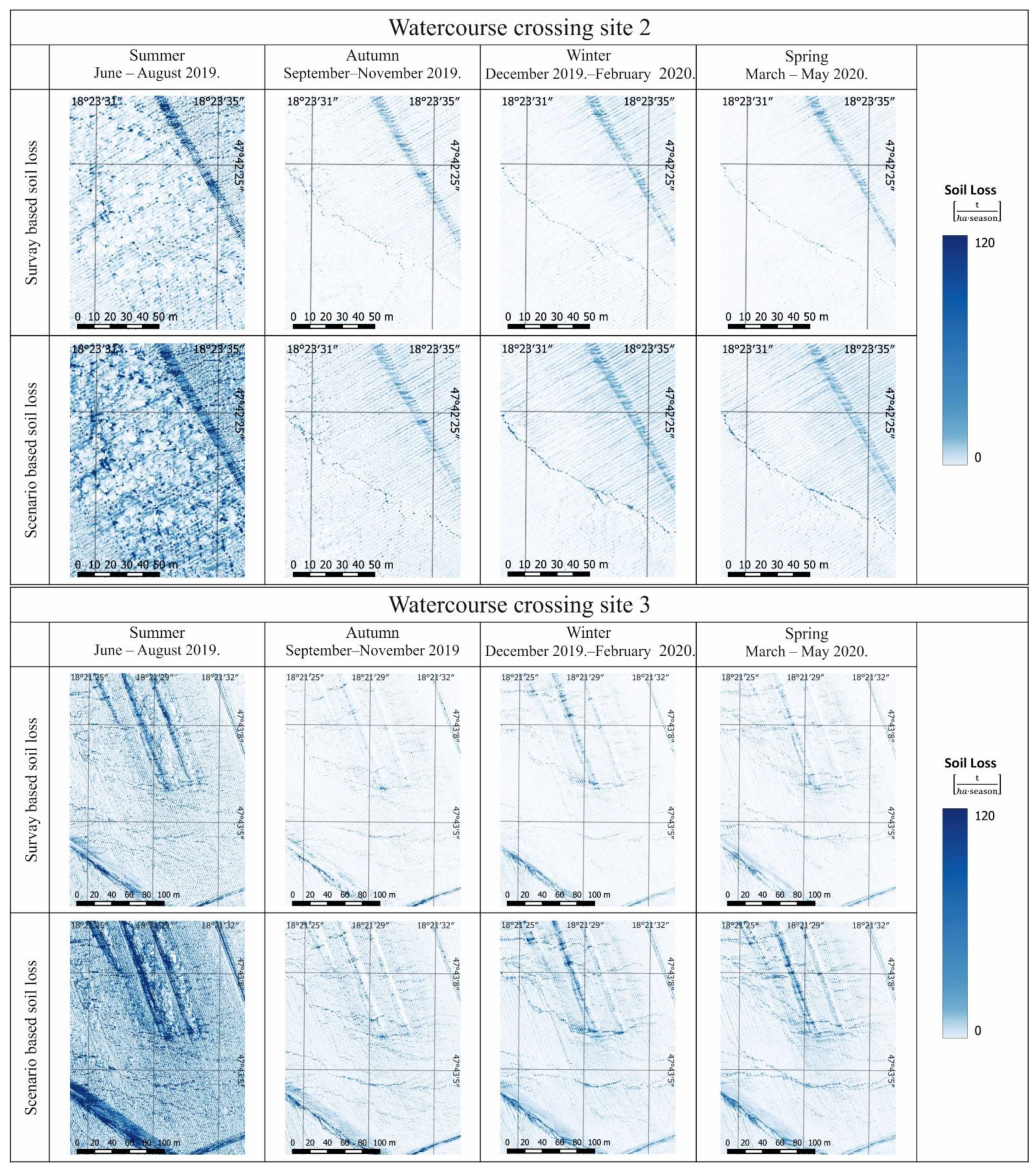
We constructed a scenario in which our aim was to investigate the erosion control effect of the land cover. In this part of the study, we paid special attention to sites 2 and 3. This was calculated by examining the importance of inter-row grass cover in terms of soil degradation at these sites.

For this scenario, a new C factor map was created in which the previously grassed areas were replaced by bare soil, i.e., the C-value was increased from 0.0564 to 1.

Table 6. Size of study sites and grassland area in ha.

Site	Season	Total Sample Area (ha)	Grassed Area (ha)
1. Elő-haraszt	Summer 2019	10.94	1.37
	Autumn 2019		3.32
	Winter 2019–2020		2.48
	Spring 2020		1.49
2. Kereszt-rét	Summer 2019	12.94	8.31
	Autumn 2019		6.49
	Winter 2019–2020		5.86
	Spring 2020		7.61
3. Göte-oldal/Korma föle	Summer 2019	39.52	23.28
	Autumn 2019		18.68
	Winter 2019–2020		16.90
	Spring 2020		16.06

shows the total size of the study sites and the amount of grassland area that changed during the modelling of the C factor. The modelled C factor was also used to estimate the extent of soil erosion.

3. Results

3.1. Seasonal Changes in Soil Erosion

For all four periods (seasons), estimated soil degradation maps were produced for each study site (Figure 5). The maps show how many tons of soil eroded per hectare and per season.

Table 7. The amount of soil erosion by season and the mean value per hectare in tons for the study sites.

Site	Season	$\mathbf{Mean} \mathbf{Soil} \mathbf{Loss} \left[\frac{\mathrm{t}}{\mathrm{h}\mathrm{a}\mathrm{·}\mathrm{s}\mathrm{e}\mathrm{a}\mathrm{s}\mathrm{o}\mathrm{n}}\right]$
1. Elő-haraszt	Summer 2019	$9.49$
	Autumn 2019	$1.09$
	Winter 2019–2020	$0.90$
	Spring 2020	$1.22$
2. Kereszt-rét	Summer 2019	$6.80$
	Autumn 2019	$0.74$
	Winter 2019–2020	$0.65$
	Spring 2020	$0.49$
3. Göte-oldal/Korma föle	Summer 2019	$16.39$
	Autumn 2019	$1.56$
	Winter 2019–2020	$1.65$
	Spring 2020	$1.81$

shows the soil loss per season and the average soil loss per hectare for each study site. In all three sample areas, soil loss was the highest in the summer period, despite the fact that this was the season with the highest plant cover. During the summer, the mean soil loss was almost always an order of magnitude different from the autumn, winter and the spring values ($6.80–16.39$ t/ha in summer and $0.65–1.65$ t/ha in winter), which is due to the heavy rainfall during the summer. In the spring measurements, the only area with lower soil loss values compared to the autumn and winter measurements was site 2, but the difference in magnitude did not change. For sites 1 and 3, spring erosion values were the highest after summer ($1.22$ and $1.81$ t/ha) due to less but more intense rainfall compared to autumn and winter.

The maximum tolerable rate of soil degradation in intensive agricultural land is 2 t/ha/year [42]. However, there exists another soil-loss tolerance rate for farmers which is less strict. According to the USLE manual, this rate is 12.5 t/ha/year [42]. By summing the seasonal results, the annual rate of soil degradation was also determined for the period under study. We indicate the areas with high risk of erosion in Figure 6. In the areas marked in red on the maps, the rate of soil loss exceeded the amount accepted in the more lenient measured. The areas of high risk were located along roads and watercourses at all sites surveyed. At site 1, the highest values were not observed in the vineyard area but in the arable fields on the two edges. At site 2, around the middle of the road from the NNW to the SSE that crosses the area, the intermittent watercourse entering the road from the SE was found to be a high risk area, which was even more pronounced along the road due to the lack of vegetation. In site 3, higher values were observed in the parcels in the north-western part called “Lófingató” and in the central part called “Göte Chardonnay”. In these areas, the vines were planted parallel to the direction of the slope. In the terraced part (upper third of the western side), the highest values were found along the terraces. The south-western part of this area was also under arable cultivation.

3.2. Effect of the Land Cover on Erosion Rates

The effect of land cover was measured using the C factor values generated in the scenario. Part of the seasonal soil loss per season estimated with this new C factor for sites 2 and 3 is shown on the maps in Figure 7.

By comparing the scenario model results with the survey maps, the amount of soil that can be protected from degradation by grassland per cell could be determined. As there was a very small area of grassland in the original condition for site 1, the smallest discrepancy between modeled and surveyed erosion was found for the site. The differences were mainly found in the area of the older vineyard parcel overhanging the study site. For the other two sites, the differences were more significant. For site 2, there was significant variation along the watercourse that crossed the site, while for site 3 there were several priority areas which are as follows: the terraced parcel; the larger watercourses; and the parcels where cultivation was not perpendicular to the slope. The seasonal variation of the study sites are summarised in

Table 8. Survey-based and modelled soil degradation rates for each study site.

	$\mathbf{Soil} \mathbf{loss} \mathbf{Rate} \left[\frac{\mathrm{t}}{\mathrm{s}\mathrm{i}\mathrm{t}\mathrm{e}\mathrm{·}\mathrm{s}\mathrm{e}\mathrm{a}\mathrm{s}\mathrm{o}\mathrm{n}}\right]$
Site		Summer	Autumn	Winter	Spring
1. Elő-haraszt	Survey	1.04 × 108	1.19 × 107	9.9 × 106	1.34× 107
	Scenario	1.23 × 108	1.76 × 107	1.27 × 107	1.4 4 × 107
2. Kereszt-rét	Survey	8.79 × 107	9.57 × 106	8.43 × 106	6.37 × 106
	Scenario	3.58 × 108	2.43 × 107	2.14 × 107	$2.00\times {10}^7$
3. Göte-oldal/Korma föle	Survey	6.48 × 108	6.11 × 107	6.52 × 107	7.13 × 107
	Scenario	1.98 × 109	1.3 × 108	1.38 × 108	1.22 × 108

.

By summing the seasonal results in the scenario, an annual soil loss estimate was also obtained (Figure 8). The results indicate that soil degradation rates would be higher in all study sites if the rows of vines were not grassed.

Table 9. Annual soil degradation and modelled annual soil degradation rates by study site.

Site	Annual Soil Loss $\left[\frac{\mathbf{t}}{\mathrm{s}\mathrm{i}\mathrm{t}\mathrm{e}\mathrm{·}\mathrm{y}\mathrm{e}\mathrm{a}\mathrm{r}}\right]$	Scenario Annual Soil Loss $\left[\frac{\mathrm{t}}{\mathrm{s}\mathrm{i}\mathrm{t}\mathrm{e}\mathrm{·}\mathrm{y}\mathrm{e}\mathrm{a}\mathrm{r}}\right]$
1. Elő-haraszt	1.39$\times {10}^8$	1.67$\times {10}^8$
2. Kereszt-rét	1.12$\times {10}^8$	4.24$\times {10}^8$
3. Göte-oldal/Korma föle	8.45$\times {10}^8$	2.37$\times {10}^9$

shows a comparison of the actual and modeled annual soil loss rates for the different sites. The calculation shows the total soil erosion values per cell per area. For site 1, this change was not significant as the area was not covered by grass at the time of the study (1.2 times). For site 2 and 3, it was much more significant (3.78 and 2.8 times, respectively). The largest change in the annual rate of soil loss occurred at site 2, where the amount of soil eroded increased by approximately 311.7 tons per year for the total area.

Average soil degradation of the study sites was calculated by using both the original and the scenario modelled values (Figure 9). At site 2, the rate of soil degradation would reach a minimum of 2.54 times and a maximum of 4.07 times, while at site 3 it would be a minimum of 1.71 times and a maximum of 3.05 times. In all cases, the largest variation was observed during the summer period.

4. Conclusions

The aim of our research was to determine the annual soil erosion rate and its seasonal variation in the most vulnerable vineyards in the northern part of the Gerecse Hill. Moreover, we produced high-resolution soil degradation maps of each study area, which could be used as tools for viticulture. Finally, 63.4 ha (in total) was surveyed in three sites near Dunaszentmiklós. The surface ground features were monitored on a seasonal time scale, thus the variation in erosion during the year could be studied.

Nowadays, several erosion models can be produced at high resolutions, aided by proximal sensing [12,43]. High resolution DEMs are able to represent small differences in the surface; thus, we can describe flow direction and accumulation in more detail [44]. In vineyards, these DEMs can help to map soil erosion in high resolution. We can capture the potential risky areas within a parcel, where nutrients disappear more quickly and there exists a chance of vine mortality.

The proximal sensing method we used was suitable for producing high resolution (10 cm/pixel) data that were processed using geoinformatics methods. In such high-resolution erosion mapping, the DoD (DEM of Difference) method is commonly used [43]; however, we were not interested in only the amount of soil loss, but also in the seasonal variation of soil loss and the significance of the effect of inter-row vegetation. That is why we used an empirical model to estimate soil erosion, the USLE model, which has been used in the past to model not only annual but also seasonal and even monthly erosion [45,46,47,48]. The model contains the effects of different influencing factors such as rainfall, topography, soil properties, vegetation cover or the type of tillage applied. Therefore, this method is suitable for investigating the effects of different vegetation cover or the variation in vegetation during the year [46,48,49,50,51].

The input data for the USLE equation used to estimate soil degradation were maps of the LS, C, and P factors based on our own surveys. Although there is a more accurate method of terrain assessment than UAV imagery (e.g., lidar), our images allowed us to determine the LS values, which show the effect of slope length and slope steepness; C values, which show the influence of different vegetation cover; and the P factor, which examines the effect of the tillage method used. The R factor was determined based on the data of two meteorological stations located near the study area. Since these stations were not specifically located in the area, the measured data used for precipitation, e.g., summer thunderstorms, may differ from the actual amount of precipitation falling in the area. However, the greater precision of these instruments made it worthwhile to use this solution rather than low-cost measuring stations that could be installed in vineyards. Finally, the spatial data set for the K factor were provided by the Institute for Soil Sciences. This was based on a complex geodatabase, but at a smaller nominal scale than the one we studied, so that the K-factor can also be considered as an approximation.

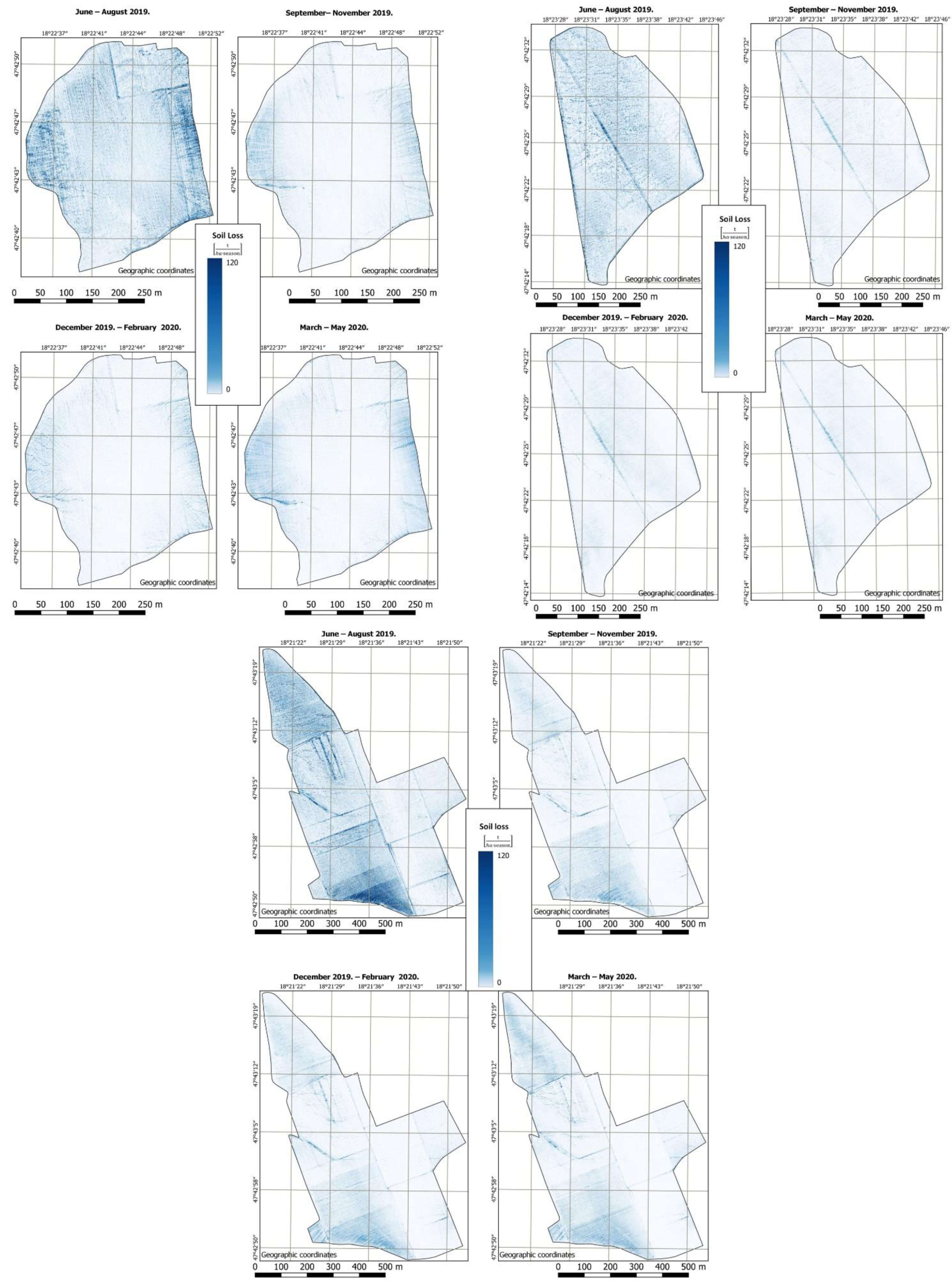
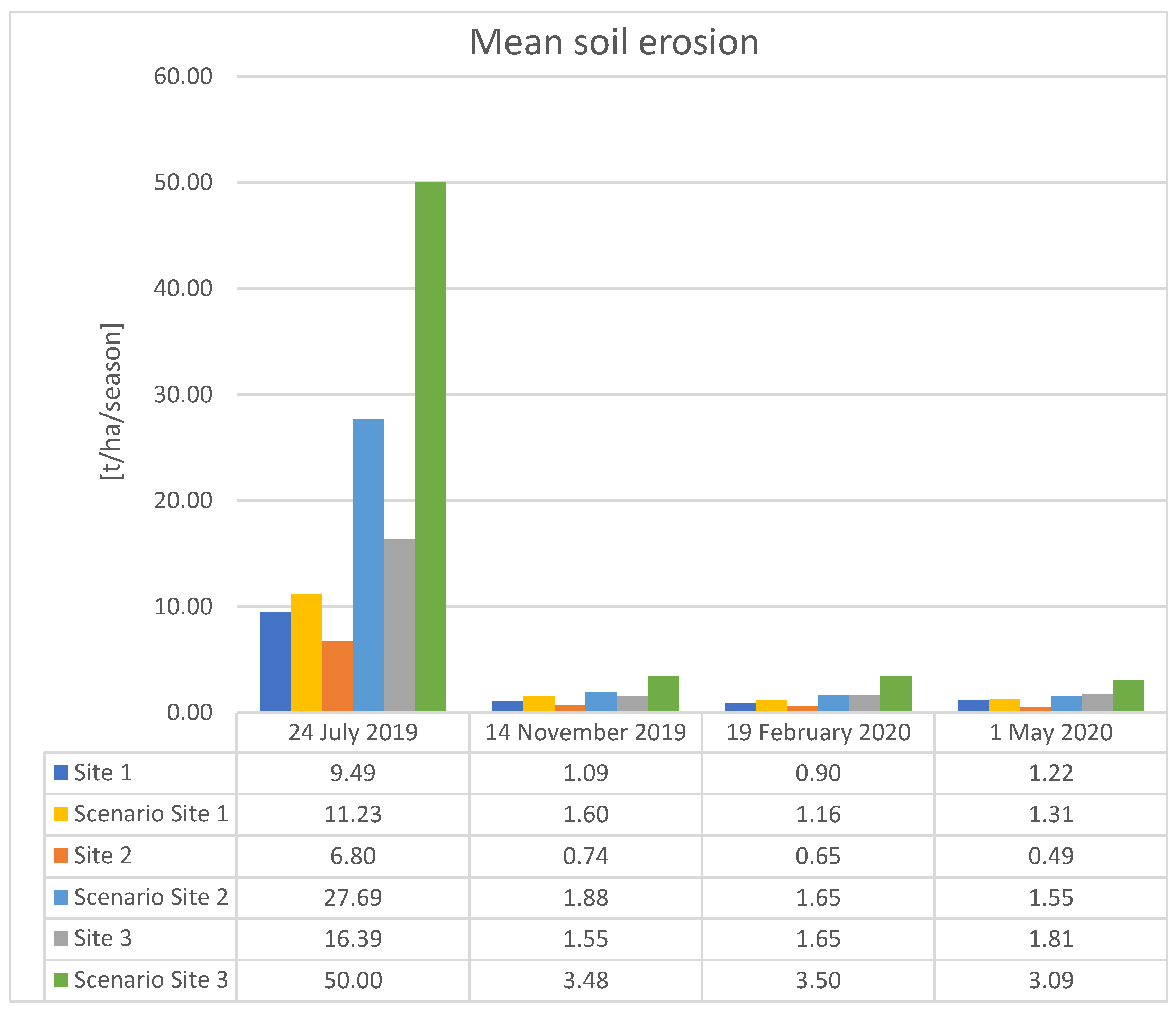
In terms of seasonal and annual soil degradation rates, it can be observed that soil degradation in the study sites varied in different seasons. In all cases, soil degradation was highest in summer. During this period, the erosion rate differed by approximately one order of magnitude compared to the other periods. In contrast, there were no significant differences between autumn and winter. In the spring period of 2020, there was no significant precipitation, so the erosion estimates were similar to the winter and autumn periods.

The maximum erosion detected in summer can be attributed to the sudden high precipitation, which can also be inferred from the R values. In contrast, the other seasons were characterised by low intensity rainfall over a long period. This seasonal variation is of course reflected not only in the effect of precipitation but also in the variation of plant cover. At the same time, high intensity rainfall has a destructive effect on plantations, which is already being observed along watercourses in the study areas. In these places, for example, fresh plantations can be washed away by water. Our results showing that the highest erosion rates occur during the wettest period of the year, in our case in the summer, are consistent with the literature.

The importance of the type of tillage used is also reflected in the results. In areas where the vines were planted in the same direction as the slope, soil erosion was higher. The predicted erosion rates were not checked quantitatively with experimental field measurements (e.g., sedimentation trap). Despite the lack of numerical verification, the high erosion values indicated on the resulting maps and the locations of the runoffs and rill erosions are consistent with the erosion traces observed in the field by local staff. (Figure 10).

The importance of inter-row grassing was also quantified in the modelling, as shown for site 2 and 3. At site 2, the minimum soil degradation rate was 2.54 times and maximum 4.07 times, while at site 3, the minimum soil degradation rate was 1.71 times and a maximum of 3.05 times if the soil was left bare. Based on the results of this study, inter-row grassing is therefore clearly recommended to reduce erosion. Erosion mapping using the proximal sensing methods presented in this study can contribute to the work towards sustainable vineyard management.