
Design and Development of Array POS for Airborne Remote Sensing Motion Compensation


1
School of Instrumentation Science and Optoelectronic Engineering, Beijing University of Aeronautics and Astronautics, Beijing 100191, China
2
Hangzhou Innovation Institute, Beihang University, Hangzhou 310051, China
*
Author to whom correspondence should be addressed.
Remote Sens. 2022, 14(14), 3420; https://doi.org/10.3390/rs14143420
Submission received: 23 May 2022
/
Revised: 6 July 2022
/
Accepted: 14 July 2022
/
Published: 16 July 2022
Abstract
:Multi-antenna airborne remote sensing systems have received more attention recently because they can realize high-resolution three-dimensional (3-D) imaging, such as array Synthetic Aperture Radar (SAR). Their high-precision imaging needs multi-antenna motion and relative motion between antennas. However, the existing facility and technology hardly meet the motion measurement precision demand of array SAR. To solve this problem, an array Position and Orientation System (POS) for airborne remote sensing motion compensation is designed and developed. It is composed of a high-precision POS, several small-size Inertial Measurement Units (IMU), and a 6-D deformation measurement system based on Fiber Bragg Grating (FBG) sensors. Firstly, the transfer alignment method based on 6-D deformation is used to measure the relative motion between array POS. Then, the motion conversion method from array POS to array SAR is presented to obtain the multi-antenna motion and relative motion between antennas. Finally, the ground experiment results identify that the accuracies of multi-antenna position, multi-antenna attitude, and flexible baseline length between antennas are superior to 3 cm, 0.01°, and 0.1 mm, respectively, which can meet the motion measurement precision demand of array SAR.

1. Introduction
For an airborne remote sensing system with a single antenna, such as Synthetic Aperture Radar (SAR), its high-precision two-dimensional (2-D) imaging needs a Position and Orientation System (POS) to provide motion compensation [1]. POS is an integrated navigation system with multiple sensors [2,3] and is composed of a high-precision Inertial Measurement Unit (IMU), a Global Navigation Satellite System (GNSS), and a POS Computer System (PCS) [4,5,6]. In recent years, on the basis of the single-antenna system, the multi-antenna airborne remote sensing system represented by array SAR has been developed and quickly become the most attractive and competitive development direction, because it can bring about all-weather three-dimensional (3-D) imaging [7,8] and includes multi-baseline interferometry [9], multi-input and multi-output [10], and tomography modes [11]. Each antenna of array SAR is installed at both wings along the length. Due to the gust, turbulence, engine vibration, and the aircraft weight variation, the wing will generate deformation, which will seriously reduce the imaging precision. Therefore, the high-precision imaging of array SAR needs not only the multi-antenna motion, but also the relative motion between antennas [12,13]. In general, the submillimeter-level baseline length precision between antennas, centimeter-level position precision of multi-antennas, and a multi-antenna attitude precision better than 0.05° are required [14]. Thus, only the POS cannot meet the motion measurement demand of array SAR.
In order to measure the multi-antenna motion and relative motion between antennas, researchers have carried out many studies. Wheeler et al. [15] used an Inertial Navigation System (INS)/Global Position System (GPS) integrated navigation system and a complex optical measurement system composed of five laser rangefinders, eight cameras, and reflectors and beacons to measure the absolute motion and relative position for dual-frequency interferometric radar, respectively. Although it can measure the absolute and relative motions, the optical measurement system is susceptible to the weather and light [16,17], which will reduce measured accuracy or even be impossible to measure. Thus, this scheme is difficult to realize all-weather remote sensing tasks with high-precision.
Aiming at this problem, distributed POS is developed to measure multi-antenna motion and relative motion for array SAR, and is composed of a high-precision POS and several IMUs [18]. Its working principle is shown as follows. Firstly, the motion of POS is obtained by INS/GNSS integrated navigation technology. Then, the motion of each IMU can be received by transfer alignment technology based on a mathematical model of deformation, taking the POS motion as the measurement vector [19]. Finally, the relative motion can be obtained by subtraction of two motions.
However, due to the complexity and uncertainty of the wing deformation, the mathematical model, such as Markov process, is hardly able to describe the actual deformation, which will restrain the transfer alignment accuracy [20]. Moreover, this transfer alignment method will be affected by the motion error of POS and reduce the accuracy. Therefore, is it is very difficult for distributed POS to meet the motion precision demand of array SAR.
Aiming at the problem that the mathematical model is not accurate, Fiber Bragg Grating (FBG) sensors are used to measure the deformation [21,22,23,24], because of the advantages of light weight, high sensitivity, and anti-electromagnetic interference [25,26,27]. Li et al. [28] established a six-dimensional (6-D) deformation measurement system based on FBG sensors and obtained encouraging experimental results in the laboratory. However, it can only provide the deformation and cannot meet the demand of multi-antenna motion.
To solve the above problems, on the basis of distributed POS, the array POS for airborne remote sensing motion compensation is designed and developed. It is composed of a high-precision master POS, several small-size Slave IMUs (SIMU), and the 6-D deformation measurement system based on FBG sensors. Thereinto, the IMU of master POS is also called Master IMU (MIMU). The working principle of array POS is shown in Figure 1. Firstly, the transfer alignment method based on 6-D deformation is used to measure the relative motion between MIMU and SIMU, and includes the relative inertial navigation algorithm, 6-D deformation method, and Kalman filter based on relative navigation. Then, the motion conversion method from array POS to array SAR is presented to obtain the multi-antenna motion and the relative motion between antennas. Finally, the ground experiment is carried out to verify the performance of array POS.
The rest of this paper is organized as follows. Section 2 introduces the component and layout of array POS, the transfer alignment method based on 6-D deformation, and the motion conversion method from array POS to array SAR. Section 3 reports the experimental equipment and results. Conclusions are drawn in Section 4.
2. Materials and Methods
2.1. Component and Layout of Array POS
Array POS is composed of a high-precision master POS including a MIMU composed of three fiber optic gyroscopes and three quartz accelerometers, a GNSS, and a PCS, several small-size SIMUs composed of three Micro Electro Mechanical System (MEMS) gyroscopes and three MEMS accelerometers, and the 6-D deformation measurement system including many FBG sensors and an FBG interrogator, as shown in Figure 2.
In Figure 2, MIMU, SIMU, GNSS, and FBG sensors as the data acquisition components are used to measure the angle velocity and acceleration at the installation position of MIMU, the angle velocity and acceleration at the installation position of SIMU, the position and velocity at the installation position of GNSS antenna, and the strain at the installation position of the FBG sensor, respectively, and the PCS and FBG interrogator are the data processing components. The volume, weight, and acquisition frequency of MIMU are 187 × 174 × 135 mm3, 4.4 kg, and 200 Hz, respectively, and those of SIMU are 70 × 64 × 17 mm3, 100 g, and 200 Hz, respectively. The gyroscope drift and accelerometer bias of MIMU are better than 0.01°/h and 10μg, respectively, and those of SIMU are better than 3°/h and 50μg, respectively. The post-processed position and attitude accuracies of the master POS are better than 3 cm and 0.005°, respectively. FBG strain sensors are carved in corning SMF-28e fibers using phase mask technology, and its strain-measured precision and acquisition frequency are 3με and 20 Hz, respectively.
In general, array SAR is installed at both wings along length. To measure the multi-antenna motion and the relative motion between antennas for array SAR, array POS also needs to be installed at both wings along length, and the layout of each part for array POS is shown in Figure 3.
In Figure 3, MIMU is installed in the cabin, and each SIMU is installed bellow both wings along length as close to each SAR antenna as possible. FBG sensors are pasted at points A, B, C, and D of each wing cross-section by epoxy glues; points A, B, and C are on the upper surface and point D is on the lower surface. To obtain a high-precision deformation, the distance between two adjacent cross-sections is less than 20 cm, and four points should be as far apart as possible [28]. FBG sensors at each wing are connected along length to form 4 FBG arrays, and the end of FBG array is connected to the FBG interrogator. Moreover, the PCS and FBG interrogator as the data processing systems are in the cabin, and a GNSS antenna is mounted at the top of the aircraft.
2.2. Transfer Alignment Method Based on 6-D Deformation
The transfer alignment is the key technology to realize relative motion measurement between MIMU and SIMU and consists of the relative inertial navigation algorithm and the Kalman filter based on relative navigation. Firstly, the relative motion is preliminarily measured by relative inertial navigation algorithm. Then, the Kalman filter based on relative navigation is established taking the 6-D deformation as the measurement vector to accurately estimate the inertial navigation error and improve the relative motion accuracy.
The relative position and attitude relationship between MIMU and SIMU is shown in Figure 4. Denoted by the body frame of MIMU, by the body frame of SIMU, and by the inertial frame. Denoted by , , , and three axes and the origin of with , respectively. Denoted by , , and the MIMU position, SIMU position, and the relative position between MIMU and SIMU, respectively.
2.2.1. Relative Inertial Navigation Algorithm
The relative inertial navigation algorithm can realize relative motion update in time domain using gyroscope and accelerometer data of MIMU and SIMU, and includes the differential equations of relative attitude, relative velocity, and relative position shown as follows:
where is the anti-symmetric matrix composed of the bracketed vector , is the angular velocity of with respect to in , and is the angular velocity of with respect to in . is the relative velocity between MIMU and SIMU, is the specific force of with respect to in , and is the specific force of with respect to in . is the relative attitude matrix from to , which is composed of Euler angles , , and around axes , , and , respectively, and can be expressed as:
By solving the numerical solution in Equation (1), the relative attitude matrix, relative velocity, and relative position can be updated. Then, according to the relative attitude matrix, the updated relative attitude can be given by:
where is the value of in the j-th column of the i-th row.
2.2.2. 6-D Deformation Method
When the aircraft is in flight, the wing will generate two plane-bending deformations and a torsion deformation due to the gust, turbulence, engine vibration, and aircraft weight variation. The bending deformations in plane and are shown in Figure 5a,b, respectively, and each plane-bending deformation is composed of a deflection, an axial displacement, and a bending angle. The torsion deformation is shown in Figure 5c and includes one torsion angle. Due to the actions of the bending and the torsion, the 6-D deformation of the wing will generate and needs to be measured by the 6-D measurement method based on FBG sensors which is composed of the strain measurement principle of the FBG sensor, the strain decoupling approach, the bending model, the torsion model, and the 6-D deformation model.
- Strain Measurement Principle of FBG Sensors
As shown in Figure 6, the FBG sensor has a selective function for different wavelength light and it reflects specific wavelengths of light and transmits all others [29]. The central wavelength of the reflected light can be expressed as:
where is the effective refractive index of the grating in the fiber core and is the grating period which varies with the strain and the temperature. Thus, the measured strain is mainly determined by both the central wavelength change and the temperature change and can be approximately expressed as:
where is the strain sensitivity coefficient and is the temperature sensitivity coefficient.
- 2
- Strain Decoupling Approach
The strain measured by the FBG sensor couples several compositions and cannot be directly used to calculate the deformation. Therefore, the strain decoupling approach is needed to improve the measured accuracy of the strain. According to the measured demands of 6-D deformation, the strains , , , and need to be decoupled from the other strain and are shown as follows:
where , , and are the strain generated by bending around neutral axis y at points , , and , respectively, and is the strain generated by bending around neutral axis z at point . , , , and are known strains measured by FBG sensors at points , , , and , respectively, and is the coefficient matrix in reference [28].
The continuous strains , , , and can be obtained by fitting the strains , , , and of each cross-section along wing length l with the quadratic polynomial.
- 3
- Bending Model
According to the principle of plane-bending deformation, the bending angle, axial displacement, and deflection generated by bending around axis at centroid of any cross-section can be obtained and given by:
where is the distance between point and neutral axis in any cross-section, , and .
After the linear superposition of and , the whole axial displacement at centroid of any cross-section can be expressed as:
- 4
- Torsion Model
According to the calculation method of torsion deformation in reference [28], the torsion angle at centroid of any cross-section, as shown in Figure 5c, can be obtained and given by:
- 5
- 6-D Deformation Model
According to the calculated axial displacement , deflections and , bending angles and , and torsion angle , the 6-D deformation at centroid of any cross-section expressed in frame can be obtained and expressed as:
where and are 3-D displacement deformation and 3-D angle deformation in frame , respectively.
According to the 6-D deformation obtained by equation (12) and the angle between frames and in plane , the 6-D deformation at centroid of any cross-section expressed in frame m can be received and expressed as:
where and are the 3-D displacement deformation and 3-D angle deformation expressed in frame , respectively.
2.2.3. Kalman Filter Based on Relative Navigation
Due to the errors of gyroscope and accelerometer, the relative inertial navigation error will drift with time, and the Kalman filter based on relative navigation is the key technology to estimate error and improve accuracy taking 6-D deformation as the measurement vector. It includes the state equation and measurement equation, which can be obtained by the relative motion error differential equations shown as follows:
where , , and are the errors of relative attitude, relative velocity, and relative position, respectively. and are constant errors of gyroscope and accelerometer from SIMU, respectively, and .
The state vector is chosen as follows:
According to the error differential Equation (14) and state vector (15), the state equation can be received and given by:
where is the system noise matrix composed of the random noise from gyroscope and accelerometer, and the system matrix and the system noise drive matrix can be described as follows:
where
The measurement vector is selected as:
where is the value of with respect to its initial state, , and are the initial relative position obtained by initial calibration. is the value of with respect to the initial state, which can be obtained by solving its relative attitude matrix with , is the initial relative attitude matrix obtained by initial calibration, and can be given by:
where is the element of in the j-th column of the i-th row.
According to the measurement vector (21) and the state vector (15), the measurement equation can be given by:
where is the measurement noise of 6-D deformation and the measurement matrix is shown as:
2.3. Motion Conversion Method from Array POS to Array SAR
Although this transfer alignment method can measure the relative motion between MIMU and SIMU, array SAR needs multi-antenna motion and relative motion between the main transmitting antenna and other receiving antennas. Thus, the motions between array POS need to be converted to those of between array SAR. Moreover, because the structure size is not infinitely small, the rigid lever-arm with shown in Figure 7 will exist between the measured center of the i-th SIMU and the phase center of the i-th antenna and needs to be compensated because it can generate the nonnegligible position error.
2.3.1. Relative Motion between Antennas
Firstly, the relative motion between MIMU and the SAR antenna can be obtained by that of between MIMU and SIMU and the rigid lever-arm, and is given by:
where and are the relative position and attitude between MIMU and the i-th antenna, respectively. and are the relative position and attitude between MIMU and the i-th SIMU. is the rigid lever-arm between the i-th SIMU and antenna and projected in the i-th SIMU body frame . is the relative attitude matrix from to , and is the amount of SAR antenna or SIMU.
Afterwards, the antenna 1 is assumed to be the main transmitting antenna, and the relative motion between antenna 1 and other receiving antennas can be obtained and given by:
where and are the relative position and the relative attitude matrix between antenna 1 and the i-th antenna, and the relative attitude can be obtained by solving and is given by:
where is the value of in the j-th column of the i-th row.
According to the relative position between antennas, the baseline length between antenna 1 and the i-th antenna can be calculated and shown as:
2.3.2. Multi-Antenna Motion
The multi-antenna motion can be obtained by the post-processed motion of the master POS and the relative motion. Firstly, the motion of antenna 1 can be given by:
where and are the position and attitude matrix of antenna 1, respectively, and is the post-processed position of master POS. is the conversion matrix from length to latitude, longitude, and height, and is the attitude matrix from to navigation frame , which can be obtained by the post-processed attitude of master POS. The attitude of antenna 1 can be obtained by solving and is given by:
where is the value of in the j-th column of the i-th row.
Then, the motion of other antennas can be given by:
where and are the position and the attitude matrix of the i-th antenna, respectively, and the attitude of the i-th antenna can be obtained by solving , which can be expressed as:
where is the value of in the k-th column of the j-th row.
3. Results
3.1. Experimental Equipment
To verify the performance of array POS, the experiment on the ground needs to be carried out. Firstly, two aluminum alloy airfoil wing models with lengths of 3 m are designed and fabricated and both wing roots are fixed on the turntable to form the experimental platform on the ground with a wingspan of 6 m. Afterwards, the array POS is established on the platform, which includes a high-precision master POS, six small-size SIMUs, and the 6-D deformation measurement system with about 120 FBG sensors and an interrogator, and the wing model pasted by FBG sensors is shown in Figure 8.
Next, the six points on the wing corresponding to SIMUs are assumed to be the SAR antennas and are pasted with the optical targets. Antenna 1 is regarded as the main transmitting antenna and other antennas are regarded as the receiving antennas. Finally, to verify the precision of multi-antenna motion and relative motion between antennas, a high-precision binocular camera, a double theodolite, and two benchmark POSs are selected as the benchmark equipment to complete the measurement of multi-antenna motion and relative motion. The experimental equipment is shown in Figure 9.
The high-precision binocular camera is produced by Xintuo 3D Technology Corporation with the XTDIC-STROBE-HR model and it can measure the 3-D position from tens of millimeters to several meters with an accuracy of better than 0.01 pixels. Its pixel is 12 million (4096 × 3000) and its field of view in the experiment is about 3000 mm×2200 mm. According to the pixel amount, the field-of-view size, and the measured precision of 0.01 pixels, the position precision of this camera is 3000/4096×0.01≈0.01 mm. The double theodolite is produced by Leica Corporation with the TM6100A and TS09 models and its angle precision is better than 1″. Moreover, a square reflector plate with multiple concentric rings is selected as the theodolite target, and the target centroid is determined by cutting the target ring with the theodolite cross, which can achieve a position measurement accuracy better than 0.03 mm. The high-precision binocular camera is used to measure the relative position between MIMU and antennas 1, 2, and 3, and the double theodolite is used to measure the relative position between MIMU and antennas 4, 5, and 6. According to and Equation (26), the relative position between antenna 1 and other antennas can be obtained and is further submitted into Equation (28) to gain the baseline length between antenna 1 and other antennas. The initial baseline length is listed in Table 1.
Moreover, the benchmark POS is produced by Beijing University of Aeronautics and Astronautics with the post-processed position, heading, pitch, and roll precision of better than 3 cm, 0.005°, 0.0025°, and 0.0025°, respectively, and its IMU is also composed of three fiber optic gyroscopes and three quartz accelerometers. Two benchmark POSs are installed below SAR antennas 1 and 6, which are taken as the position and attitude benchmarks of antennas 1 and 6.
3.2. Experiment Results
Due to the gust, turbulence, engine vibration, and aircraft weight variation in flight, the wing will generate deformation and the deformation usually includes the constant and vibration components. Therefore, in this experiment, the left wing is used to simulate the vibration deformation by applying static load at the wing tip and the right wing is used to simulate the constant deformation by applying pulse load at the wing tip. This experiment is repeated three times with different loads for about 3 min each time and the experimental process is shown in Table 2.
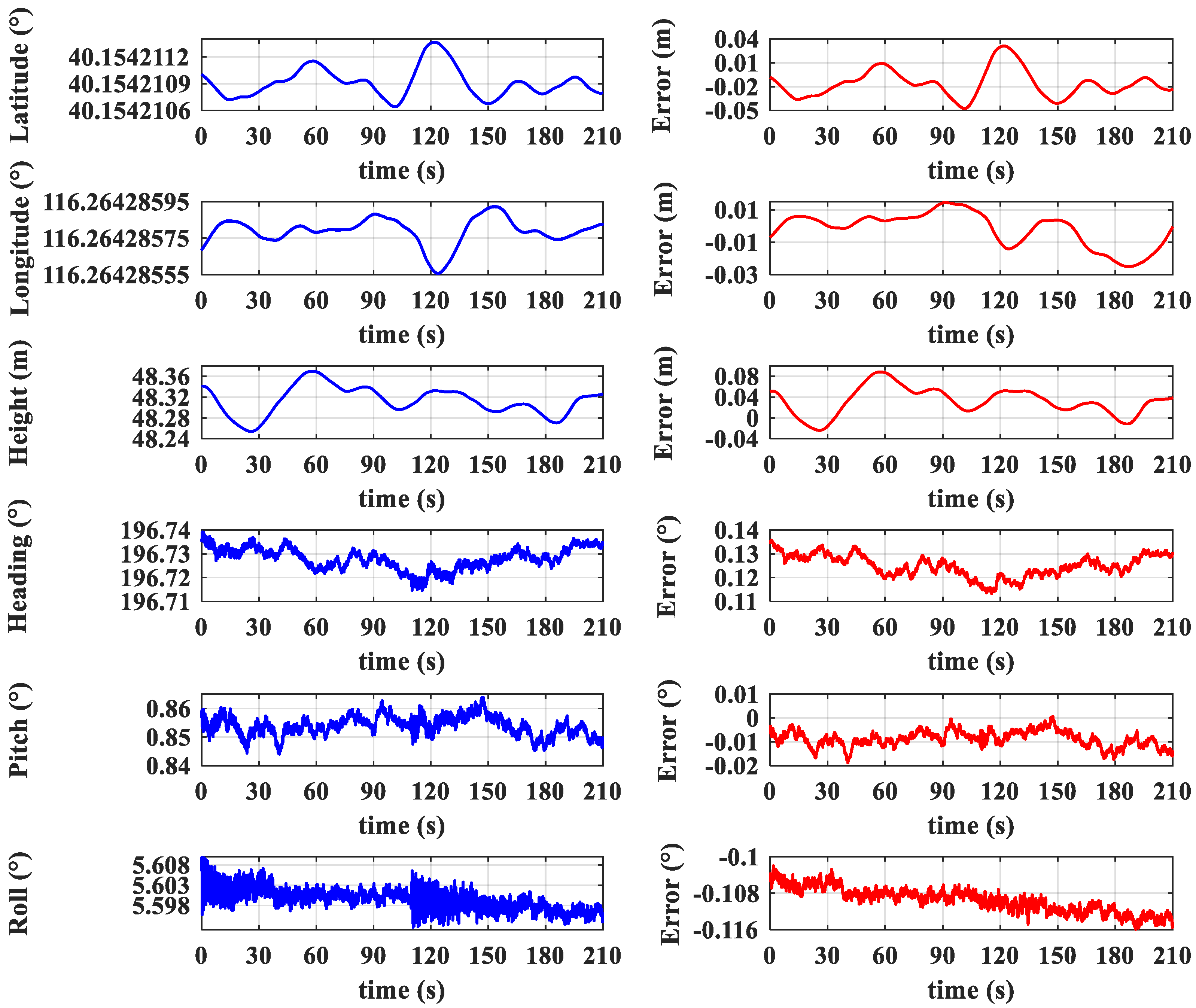
It can be seen from Table 2 that the load weight increases gradually with the loading times and the deformation also increases correspondingly. The maximum deformation occurs in the third experiment and the maximum peak-to-peak value of displacement is over 10 cm. In the third experiment, the measured values and errors of relative position and flexible baseline length between antenna 1 and other antennas are calculated and shown in Figure 10, Figure 11, Figure 12, Figure 13 and Figure 14, and those of position and attitude for antennas 1 and 6 are calculated and shown in Figure 15 and Figure 16.
To quantitatively analyze the precision of array POS, the standard deviation (STD) of error is calculated three times and the maximum value is taken as the final precision of array POS. The error statistical results of relative motion between antennas are shown in Table 3 and those of multi-antenna motion are shown in Table 4.
It can be seen from Figure 10, Figure 11, Figure 12, Figure 13 and Figure 14 and Table 3 that array POS has a great performance on relative motion measurement and the measurement accuracies of relative position and flexible baseline length between antennas are better than 0.5 mm and 0.1 mm under the maximum flexible baseline length of 5.6 m, respectively, which can meet the demands of submillimeter-level baseline length for array SAR.
4. Conclusions
In this article, aiming at the high-precision measurement problem of the multi-antenna motion and the relative motion between antennas for array SAR high-resolution 3-D imaging, an array POS for airborne remote sensing motion compensation is designed and developed and is composed of a high-precision master POS, several small-size SIMUs, and the 6-D deformation measurement system based on FBG sensors. The relative motion between antennas and multi-antenna motion can be obtained by the transfer alignment technology and the motion conversion method. The ground experiment results show that array POS can effectively measure the multi-antenna motion and relative motion, the accuracies of flexible baseline length between antennas are superior to 0.1 mm, and those of multi-antenna position and attitude are better than 3 cm and 0.01°, respectively. In a word, the designed and developed array POS can meet the compensation precision demands of multi-antenna motion and relative motion for array SAR. However, the above experimental results are obtained in an ideal laboratory environment and may be a little different from the measurement results in flight, because the actual wing structure and the flight environment are different from this experiment in the laboratory to some extent.
In the future, we will apply array POS to the actual remote sensing of array SAR and we also believe that array POS can play a great role and make a big contribution to array SAR for high-resolution 3-D imaging.
Author Contributions
Conceptualization, C.Q.; methodology, C.Q.; software, C.Q.; validation, C.Q. and J.L.; formal analysis, C.Q., J.L., J.B. and Z.Z.; investigation, J.L.; resources, J.L.; data curation, J.L. and Z.Z.; writing—original draft preparation, C.Q.; writing—review and editing, C.Q. and J.L.; visualization, J.B.; supervision, J.L. and Z.Z.; project administration, Z.Z.; funding acquisition, J.L. All authors have read and agreed to the published version of the manuscript.
Funding
This research was funded by the National Natural Science Foundation of China under Grant 61722103, Grant 62173019, Grant 61973020, and Grant 61873019, and, in part, by the Beijing Natural Science Foundation under Grant 4222047.
Data Availability Statement
Not applicable.
Conflicts of Interest
The authors declare no conflict of interest.
References
- Zhu, Z.; Li, C.; Zhou, X. An Accurate High-Order Errors Suppression and Cancellation Method for High-Precision Airborne POS. IEEE Trans. Geosci. Remote Sens. 2018, 56, 5357–5367. [Google Scholar] [CrossRef]
- Artés, F.; Hutton, J. GPS and Inertial Navigation-Delivering. GEOconnexion Int. Mag. 2005, 4, 52–53. [Google Scholar]
- Jiang, S.; Jiang, W. On-Board GNSS/IMU Assisted Feature Extraction and Matching for Oblique UAV Images. Remote Sens. 2017, 9, 813. [Google Scholar] [CrossRef] [Green Version]
- Scheninger, B.M.; Hutton, J.J.; McMillan, J.C. Low Cost Inertial/GPS Integrated Position and Orientation System for Marine Applications. IEEE Aerosp. Electron. Syst. Mag. 1997, 12, 15–19. [Google Scholar] [CrossRef]
- Fang, J.; Chen, L.; Yao, J. An Accurate Gravity Compensation Method for High-Precision Airborne POS. IEEE Trans. Geosci. Remote Sens. 2014, 52, 4564–4573. [Google Scholar] [CrossRef]
- Reulke, R.; Wehr, A.; Griesbach, D. Mobile Panoramic Mapping Using CCD-Line Camera and Laser Scanner with Integrated Position and Orientation System. In Imaging beyond the Pinhole Camera; Daniilidis, K., Klette, R., Eds.; Springer: Dordrecht, The Netherlands, 2006; Volume 33, pp. 165–183. [Google Scholar]
- Li, X.; Zhang, F.; Liang, X.; Li, Y.; Guo, Q.; Wan, Y.; Bu, X.; Liu, Y. Fourfold Bounce Scattering-Based Reconstruction of Building Backs Using Airborne Array TomoSAR Point Clouds. Remote Sens. 2022, 14, 1937. [Google Scholar] [CrossRef]
- Tan, K.; Wu, S.; Liu, X.; Fang, G. Omega-K Algorithm for Near-Field 3-D Image Reconstruction Based on Planar SIMO/MIMO Array. IEEE Trans. Geosci. Remote Sens. 2019, 57, 2381–2394. [Google Scholar] [CrossRef]
- Zhu, X.; Wang, Y.; Montazeri, S.; Ge, N. A Review of Ten-Year Advances of Multi-Baseline SAR Interferometry Using TerraSAR-X Data. Remote Sens. 2018, 10, 1374. [Google Scholar] [CrossRef] [Green Version]
- Yang, G.; Li, C.; Wu, S.; Zheng, S.; Liu, X.; Fang, G. Phase Shift Migration with Modified Coherent Factor Algorithm for MIMO-SAR 3D Imaging in THz Band. Remote Sens. 2021, 13, 4701. [Google Scholar] [CrossRef]
- Li, X.; Zhang, F.; Li, Y.; Guo, Q.; Wan, Y.; Bu, X.; Liu, Y.; Liang, X. An Elevation Ambiguity Resolution Method Based on Segmentation and Reorganization of TomoSAR Point Cloud in 3D Mountain Reconstruction. Remote Sens. 2021, 13, 5118. [Google Scholar] [CrossRef]
- Franceschetti, G.; Iodice, A.; Maddaluno, S.; Riccio, D. Effect of Antenna Mast Motion on X-SAR/SRTM Performance. IEEE Trans. Geosci. Remote Sens. 2000, 38, 2361–2372. [Google Scholar] [CrossRef]
- Wang, B.; Xiang, M.; Chen, L. Motion Compensation on Baseline Oscillations for Distributed Array SAR by Combining Interferograms and Inertial Measurement. IET Radar Sonar Navig. 2017, 11, 1285–1291. [Google Scholar] [CrossRef]
- Li, D.; Teng, X.; Pan, Z. The Concept and Applications of Distributed POS. J. Radars 2014, 2, 400–405. [Google Scholar] [CrossRef]
- Wheeler, K.; Hensley, S. The GeoSAR Airborne Mapping System. In Proceedings of the Record of the IEEE 2000 International Radar Conference, Alexandria, VA, USA, 12 May 2000; pp. 831–835. [Google Scholar]
- Iwasaki, Y. A Method of Robust Moving Vehicle Detection for Bad Weather Using an Infrared Thermography Camera. In Proceedings of the 2008 International Conference on Wavelet Analysis and Pattern Recognition, Hong Kong, China, 30–31 August 2008; pp. 86–90. [Google Scholar]
- Boukhriss, R.R. Moving Object Detection under Different Weather Conditions Using Full-Spectrum Light Sources. Pattern Recognition Letters 2020, 129, 205–212. [Google Scholar] [CrossRef]
- Zou, S.; Li, J.; Lu, Z.; Liu, Q.; Fang, J. A Nonlinear Transfer Alignment of Distributed POS Based on Adaptive Second-Order Divided Difference Filter. IEEE Sens. J. 2018, 18, 9612–9618. [Google Scholar] [CrossRef]
- Lu, Z.; Fang, J.; Liu, H.; Gong, X.; Wang, S. Dual-Filter Transfer Alignment for Airborne Distributed POS Based on PVAM. Aerospace Sci. Technol. 2017, 71, 136–146. [Google Scholar] [CrossRef]
- Gong, X.; Chen, L.; Fang, J.; Liu, G. A Transfer Alignment Method for Airborne Distributed POS with Three-Dimensional Aircraft Flexure Angles. Sci. China Inf. Sci. 2018, 61, 092204. [Google Scholar] [CrossRef] [Green Version]
- Pak, C. Wing Shape Sensing from Measured Strain. AIAA J. 2016, 54, 1068–1077. [Google Scholar] [CrossRef] [Green Version]
- Freydin, M.; Rattner, M.K.; Raveh, D.E.; Kressel, I.; Davidi, R.; Tur, M. Fiber-Optics-Based Aeroelastic Shape Sensing. AIAA J. 2019, 57, 5094–5103. [Google Scholar] [CrossRef]
- Klotz, T.; Pothier, R.; Walch, D.; Colombo, T. Prediction of the Business Jet Global 7500 Wing Deformed Shape Using Fiber Bragg Gratings and Neural Network. Results Eng. 2021, 9, 100190. [Google Scholar] [CrossRef]
- Kefal, A.; Tabrizi, I.E.; Yildiz, M.; Tessler, A. A Smoothed IFEM Approach for Efficient Shape-Sensing Applications: Numerical and Experimental Validation on Composite Structures. Mech. Syst. Signal. Process. 2021, 152, 107486. [Google Scholar] [CrossRef]
- Mieloszyk, M.; Majewska, K.; Zywica, G.; Kaczmarczyk, T.Z.; Jurek, M.; Ostachowicz, W. Fibre Bragg Grating Sensors as a Measurement Tool for an Organic Rankine Cycle Micro-Turbogenerator. Measurement 2020, 157, 107666. [Google Scholar] [CrossRef]
- El-Gammal, H.M.; Ismail, N.E.; Rizk, M.R.M.; Aly, M.H. Strain Sensing in Underwater Acoustics with a Hybrid π-Shifted FBG and Different Interrogation Methods. Opt Quant. Electron. 2022, 54, 226. [Google Scholar] [CrossRef]
- Deepa, S.; Das, B. Interrogation Techniques for π-Phase-Shifted Fiber Bragg Grating Sensor: A Review. Sens. Actuat. A Phys. 2020, 315, 112215. [Google Scholar] [CrossRef]
- Li, J.; Qu, C.; Zhu, Z.; Gong, X.; Sun, Y.; Li, Y.; Chen, Z. Six-Dimensional Deformation Measurement of Distributed POS Based on FBG Sensors. IEEE Sens. J. 2021, 21, 7849–7856. [Google Scholar] [CrossRef]
- Fajkus, M.; Kovar, P.; Skapa, J.; Nedoma, J.; Martinek, R.; Vasinek, V. Design of Fiber Bragg Grating Sensor Networks. IEEE Trans. Instrum. Meas. 2022, 71, 1–11. [Google Scholar] [CrossRef]
Figure 1.
Working principle of array POS.
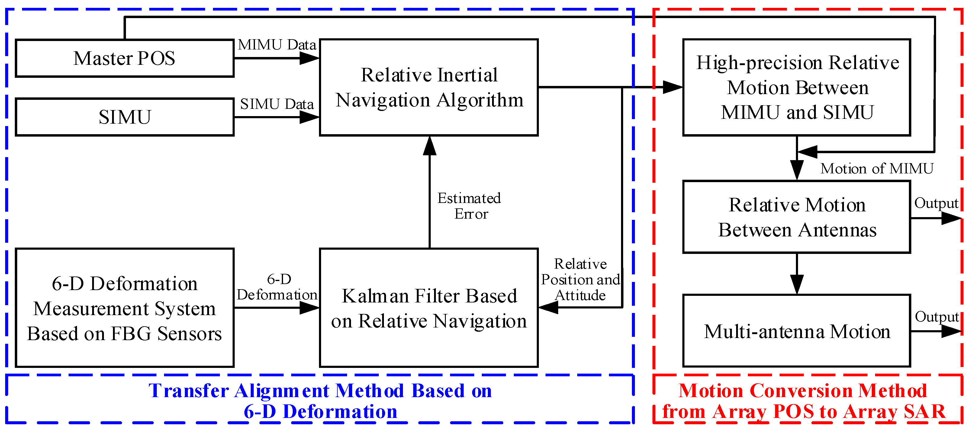
Figure 2.
Component of array POS.
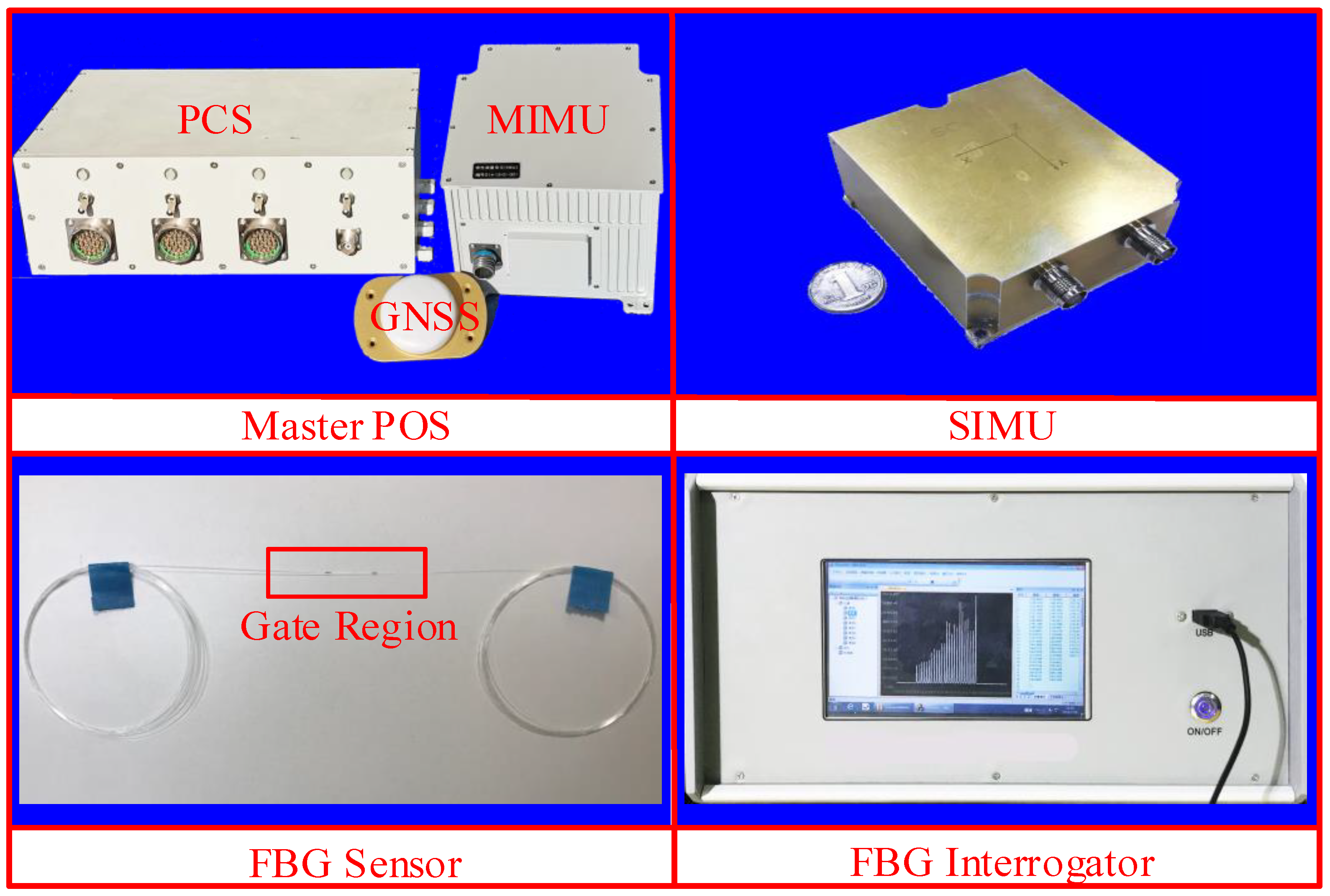
Figure 3.
Layout of array POS.
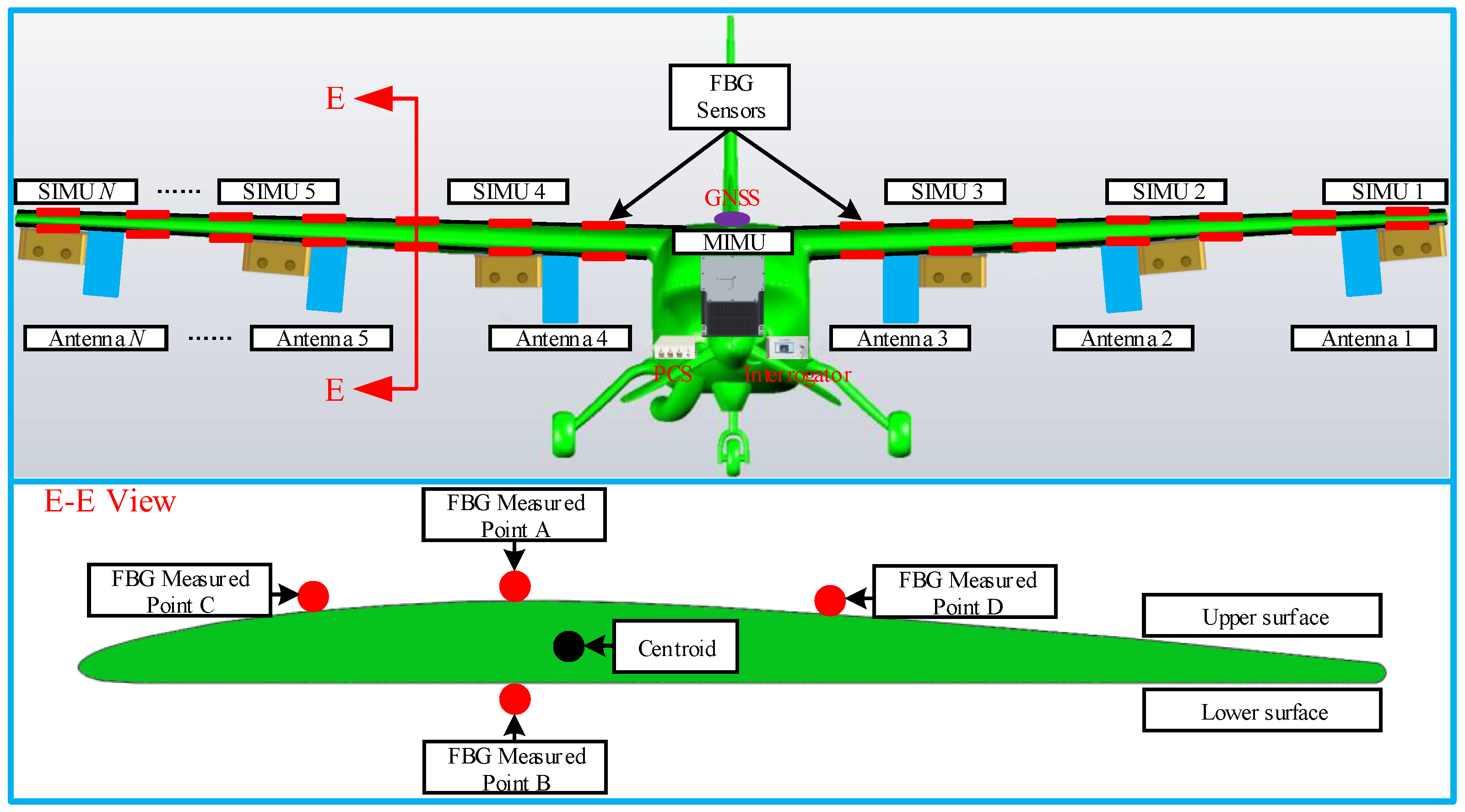
Figure 4.
Relative position and attitude relationship between MIMU and SIMU.

Figure 5.
Bending and torsion of wing. (a) Bending in plane; (b) bending in plane; (c) torsion around axis.
Figure 5.
Bending and torsion of wing. (a) Bending in plane; (b) bending in plane; (c) torsion around axis.
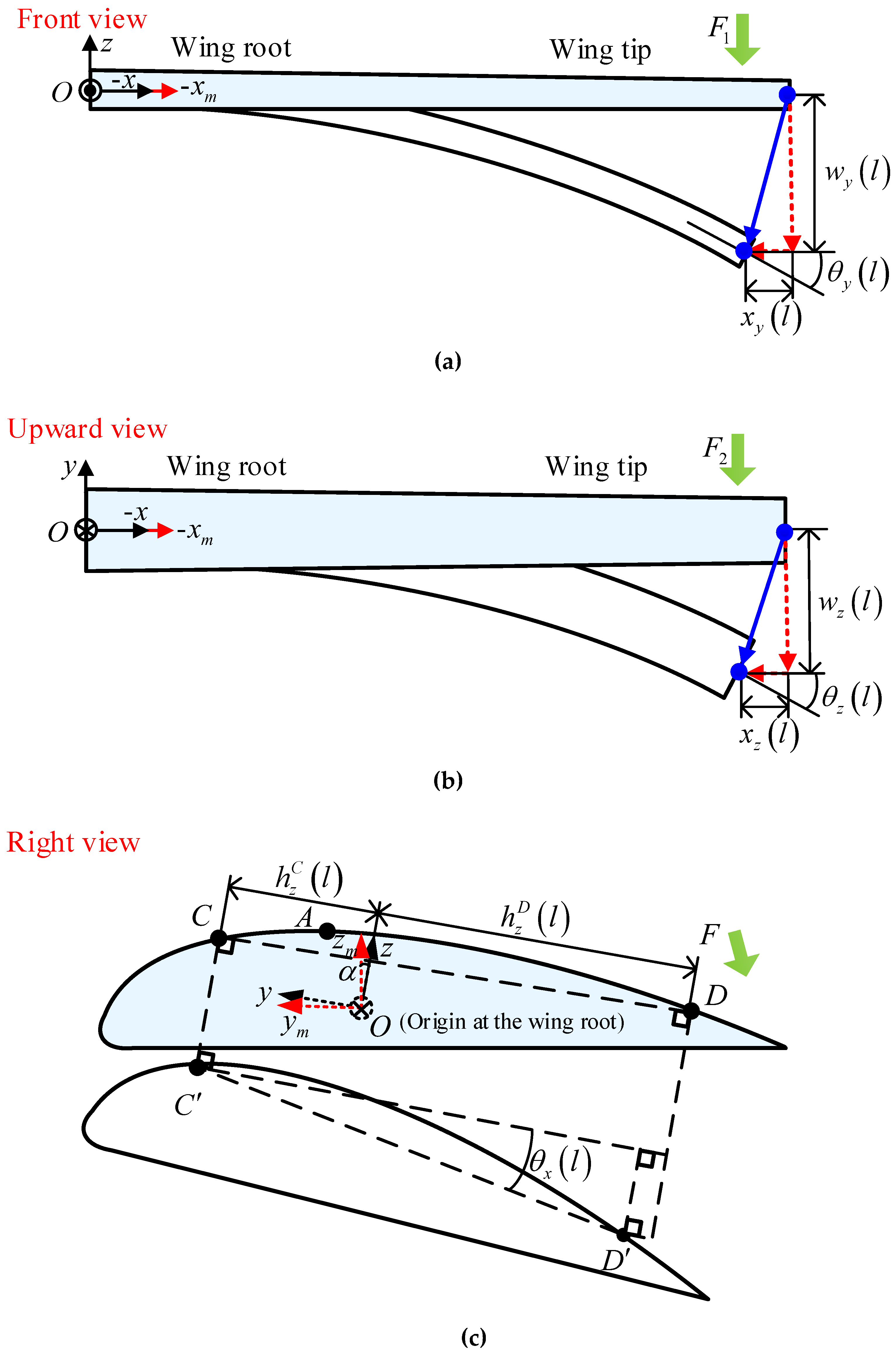
Figure 6.
Principle of FBG sensor.

Figure 7.
Rigid lever-arm between SIMU and SAR antenna.

Figure 8.
Wing model pasted by FBG sensors.
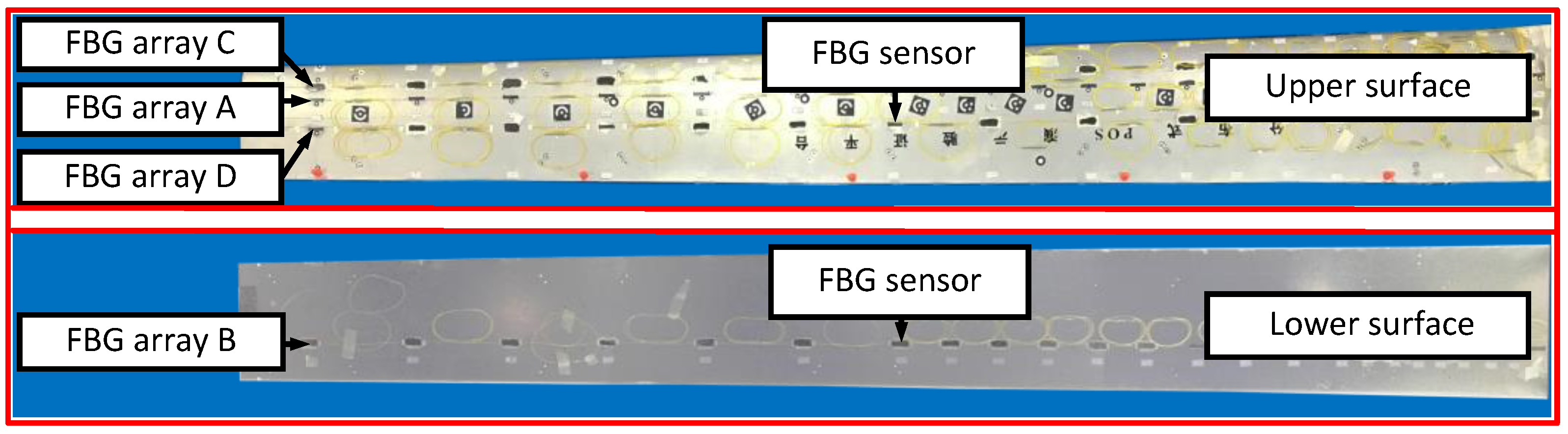
Figure 9.
Experimental equipment on the ground.
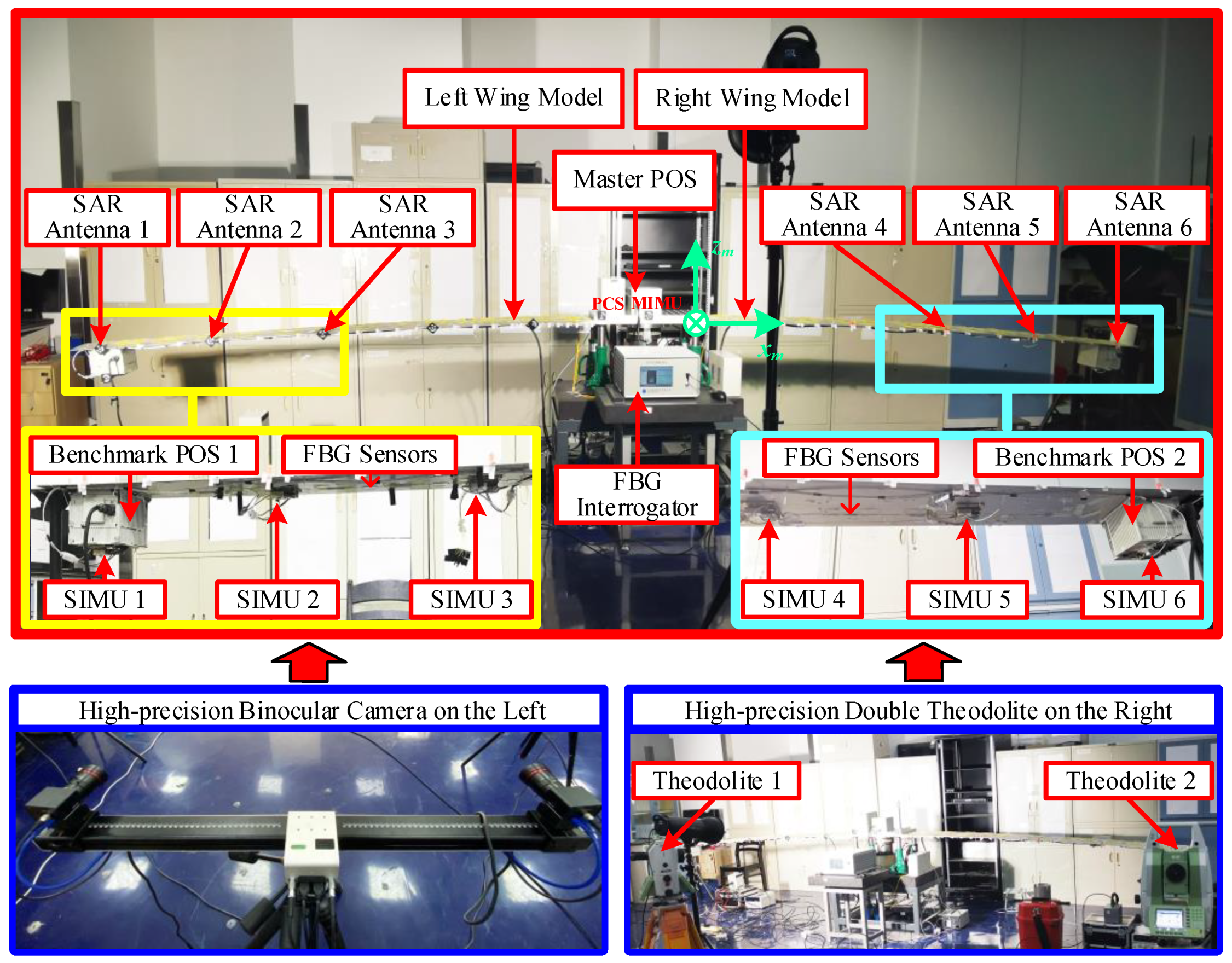
Figure 10.
Measured values and errors of relative position and baseline length between antennas 1 and 2.
Figure 10.
Measured values and errors of relative position and baseline length between antennas 1 and 2.

Figure 11.
Measured values and errors of relative position and baseline length between antennas 1 and 3.
Figure 11.
Measured values and errors of relative position and baseline length between antennas 1 and 3.
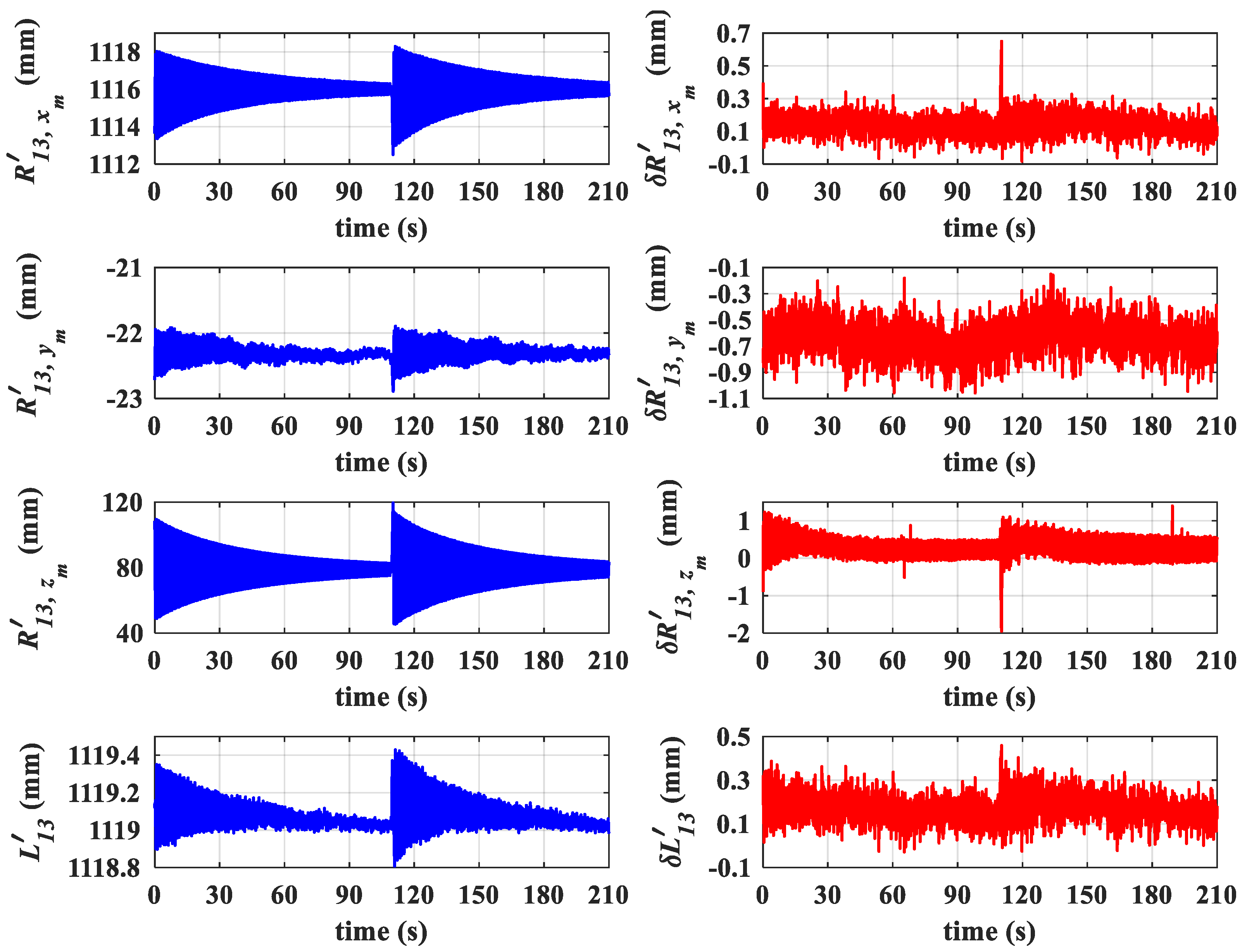
Figure 12.
Measured values and errors of relative position and baseline length between antennas 1 and 4.
Figure 12.
Measured values and errors of relative position and baseline length between antennas 1 and 4.
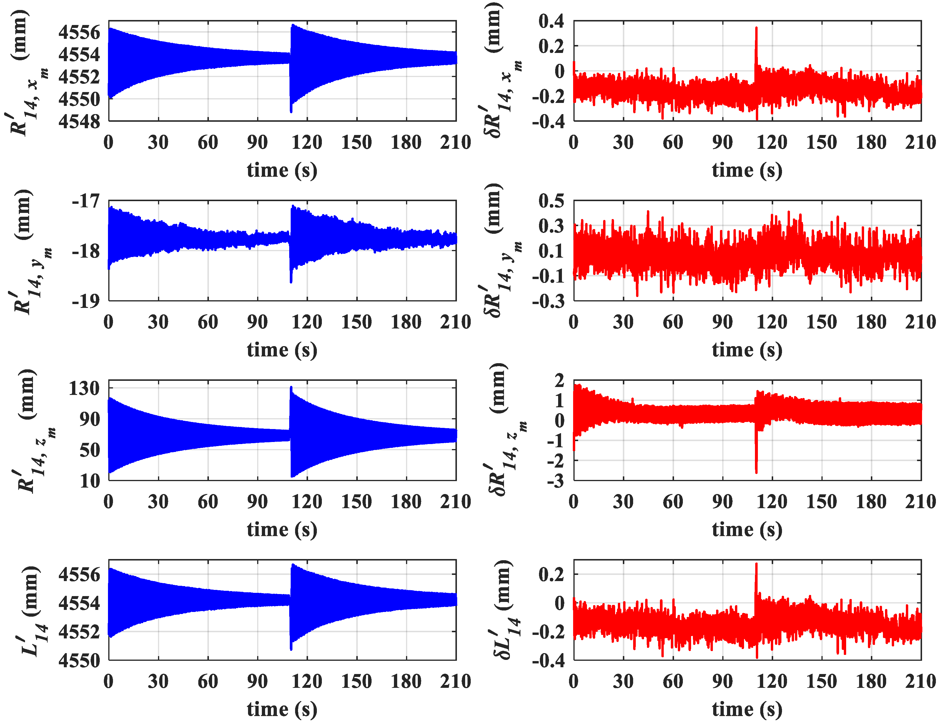
Figure 13.
Measured values and errors of relative position and baseline length between antennas 1 and 5.
Figure 13.
Measured values and errors of relative position and baseline length between antennas 1 and 5.

Figure 14.
Measured values and errors of relative position and baseline length between antennas 1 and 6.
Figure 14.
Measured values and errors of relative position and baseline length between antennas 1 and 6.
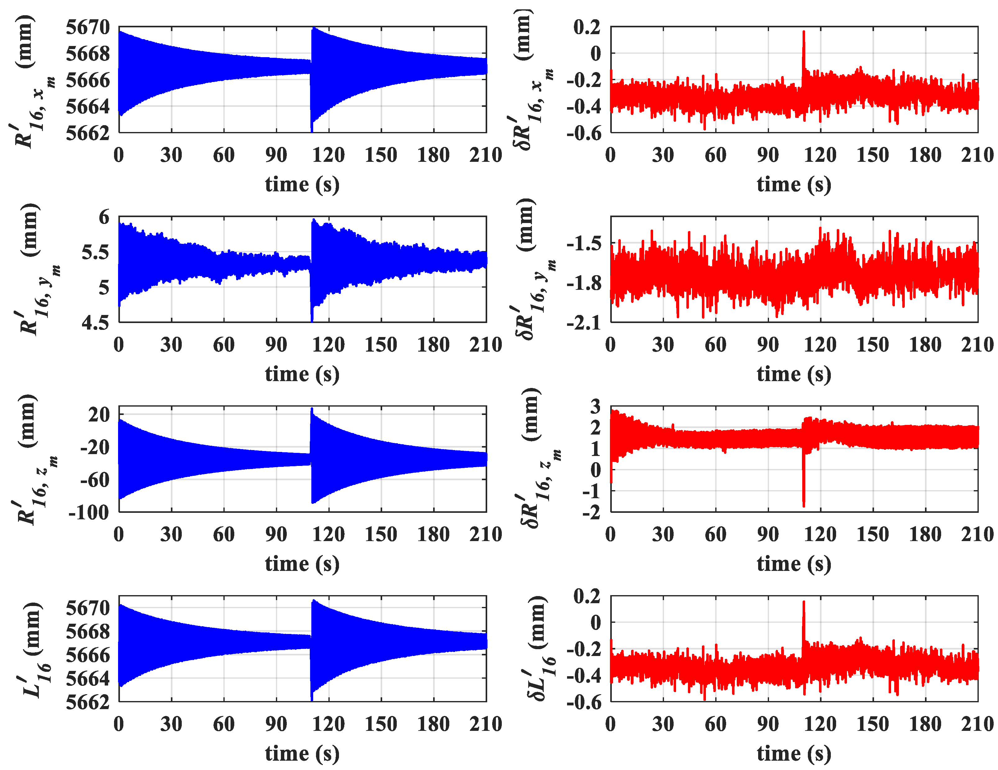
Figure 15.
Measured values and errors of position and attitude for antenna 1.

Figure 16.
Measured values and errors of position and attitude for antenna 6.

Table 1.
Initial baseline length between antenna 1 and other antennas.
| Antennas | 1 and 2 | 1 and 3 | 1 and 4 | 1 and 5 | 1 and 6 |
|---|---|---|---|---|---|
| Initial baseline length (m) | 0.5 | 1.1 | 4.5 | 5.1 | 5.6 |
Table 2.
Experimental Process.
| Loading steps | 1st | 2nd | 3rd |
|---|---|---|---|
| Right wing (Static load) | 1 kg | 3 kg | 5 kg |
| Left wing (Pulse load) | 1 kg (twice) | 3 kg (twice) | 5 kg (twice) |
| Times | 210 s | 160 s | 210 s |
Table 3.
Error statistical results of relative motion between antennas.
| Antennas | Relative Position (mm) | Baseline Length (mm) | |||
|---|---|---|---|---|---|
| 1st | 1 and 2 | 0.05 | 0.11 | 0.1 | 0.05 |
| 1 and 3 | 0.05 | 0.11 | 0.17 | 0.05 | |
| 1 and 4 | 0.05 | 0.09 | 0.26 | 0.05 | |
| 1 and 5 | 0.05 | 0.08 | 0.26 | 0.05 | |
| 1 and 6 | 0.05 | 0.09 | 0.26 | 0.05 | |
| 2nd | 1 and 2 | 0.06 | 0.12 | 0.14 | 0.06 |
| 1 and 3 | 0.05 | 0.12 | 0.24 | 0.06 | |
| 1 and 4 | 0.06 | 0.09 | 0.33 | 0.06 | |
| 1 and 5 | 0.06 | 0.09 | 0.31 | 0.06 | |
| 1 and 6 | 0.06 | 0.08 | 0.3 | 0.06 | |
| 3rd | 1 and 2 | 0.07 | 0.12 | 0.18 | 0.06 |
| 1 and 3 | 0.06 | 0.13 | 0.28 | 0.06 | |
| 1 and 4 | 0.06 | 0.09 | 0.41 | 0.06 | |
| 1 and 5 | 0.06 | 0.09 | 0.39 | 0.06 | |
| 1 and 6 | 0.07 | 0.09 | 0.38 | 0.07 | |
| Maximum | 0.07 | 0.13 | 0.41 | 0.07 | |
Table 4.
Error statistical results of multi-antenna motion.
| Antenna | Position (m) | Attitude (°) | |||||
|---|---|---|---|---|---|---|---|
| Latitude | Longitude | Height | Heading | Pitch | Roll | ||
| 1st | 1 | 0.01 | 0.01 | 0.01 | 0.004 | 0.003 | 0.002 |
| 6 | 0.01 | 0.01 | 0.01 | 0.008 | 0.003 | 0.002 | |
| 2nd | 1 | 0.01 | 0.01 | 0.03 | 0.006 | 0.006 | 0.007 |
| 6 | 0.01 | 0.01 | 0.02 | 0.004 | 0.003 | 0.001 | |
| 3rd | 1 | 0.02 | 0.01 | 0.03 | 0.006 | 0.007 | 0.008 |
| 6 | 0.02 | 0.01 | 0.03 | 0.005 | 0.003 | 0.003 | |
| Maximum | 0.02 | 0.01 | 0.03 | 0.008 | 0.007 | 0.008 | |
Publisher’s Note: MDPI stays neutral with regard to jurisdictional claims in published maps and institutional affiliations. |
© 2022 by the authors. Licensee MDPI, Basel, Switzerland. This article is an open access article distributed under the terms and conditions of the Creative Commons Attribution (CC BY) license (https://creativecommons.org/licenses/by/4.0/).
Share and Cite
MDPI and ACS Style
Qu, C.; Li, J.; Bao, J.; Zhu, Z. Design and Development of Array POS for Airborne Remote Sensing Motion Compensation. Remote Sens. 2022, 14, 3420. https://doi.org/10.3390/rs14143420
AMA Style
Qu C, Li J, Bao J, Zhu Z. Design and Development of Array POS for Airborne Remote Sensing Motion Compensation. Remote Sensing. 2022; 14(14):3420. https://doi.org/10.3390/rs14143420
Chicago/Turabian StyleQu, Chunyu, Jianli Li, Junfang Bao, and Zhuangsheng Zhu. 2022. "Design and Development of Array POS for Airborne Remote Sensing Motion Compensation" Remote Sensing 14, no. 14: 3420. https://doi.org/10.3390/rs14143420
Note that from the first issue of 2016, this journal uses article numbers instead of page numbers. See further details here.