Analysis of the 10–20-Day Intraseasonal Oscillation in the Indian Ocean Using Surface Winds

Abstract

The 10–20-day mode of surface wind is examined in the Indian Ocean, with special reference to the Arabian Sea, Bay of Bengal, equatorial, southern, and southeastern Indian Ocean during a strong (1994), weak (2002), and normal (1995) southwest monsoon season. Results indicate the 10–20-day mode of surface winds in the Bay of Bengal, southern Indian Ocean, and southeastern Indian Ocean is more energetic than in other regions. The strongest 10–20-day signal is found to be in the southeastern Indian Ocean, where 45% of surface wind variability can be explained by this mode during a strong monsoon year. Composite analysis based on a time series in this region revealed a positive surface wind anomaly that appears at 60°E, centered on 15°S, and propagates zonally eastward to 90°E before reflecting back to propagate westward and then disperse off the coast of Madagascar. It is proposed that this oscillating positive wind anomaly is a feature of the southernmost cell of the 10–20-day convective double-cell structure that has extended farther south into the southern Indian Ocean and that this mode connects the northern and southern Indian Ocean through surface winds and atmospheric convection through the motion of the linked double-cell structure.

1. Introduction

Every year, from the end of May through September, India experiences a massive influx of moisture and, consequently, precipitation known as the southwest monsoon. With over a billion residents and much of India’s agriculture largely dependent on rains from the monsoon, forecasting and characterizing it has become a large area of study in the earth sciences over the last several decades. Intraseasonal oscillations (ISOs) are often overlooked in comparison to larger-scale phenomena, such as El Niño and the Southern Oscillation (ENSO), in monsoon research. Intraseasonal oscillations operate on a much smaller scale, and thus research into them has been limited. One exception, and the one that has received the lion’s share of attention, is the Madden–Julian Oscillation (MJO) because it impacts weather and climate globally [1].

Intraseasonal oscillations that are not the MJO are often overlooked even though they are critically important to tropical and monsoonal dynamics. The 10–20-day quasi-biweekly mode is characterized by a westward propagating system in the Bay of Bengal that consists of a meridional double-cell structure (Figure 1). This variability is seen in outgoing longwave radiation (OLR), winds at 850 hPa or 200 hPa, and precipitation [2,3,4,5,6,7,8]. Although the system has its origins as a breaking Rossby wave in the upper atmosphere in the North Pacific [6], this system propagates westward into the Bay of Bengal where it becomes the northern cell of a larger double-cell structure (black circles in Figure 1) [3,4,5,6,7,8], where the northernmost cell of this structure is found to be centered between 15°N and 20° and the southernmost cell is centered between the equator and 5°S and is generated by a mixed Rossby–gravity (MRG) wave in the equatorial Bay of Bengal [8] (Figure 1). The vertical structure of the double-cell has a local Hadley circulation that links the atmospheric circulations of the two cells like interlocking gears and ties their motions together [3]. The entire structure propagates westward, with the northern cell propagating along the monsoon trough and delivering significant rainfall that contributes to the active (flood) phase of the monsoon [4]. The structure is found to be similar to that of a northward translated equatorial Rossby wave centered at 5°N [3]. This convectively coupled equatorial Rossby wave is driven unstable by moist convective feedbacks when translated north of the equator, where absolute vorticity is equal to zero at the equator [4]. Kikuchi and Wang (2009) were able to identify the source of the equatorial Rossby waves as convection over the western Pacific Warm Pool and further break down the exact sequence of events leading to the 10–20-day mode observed during the southwest monsoon [5].

The 10–20-day mode captured by surface winds in the Indian Ocean has thus far not been the focus of much research, particularly during strong and weak monsoons [8,9]. The goal of this research is to characterize the 10–20-day mode in surface wind during various monsoon regimes in regions within the Indian Ocean and to analyze the varying dynamic responses within these basins. This manuscript is organized as follows: Section 2 presents the materials and methods used (i.e., the method for identifying the 10–20-day signal). Section 3 shows the magnitude of the 10–20-day signal compared to the unfiltered winds, examines the variance explained by the 10–20-day signal, and demonstrates that the southern portion of the signal propagates across the Indian Ocean and modulates the northern circulation which stays over the Bay of Bengal. A composite analysis clearly demonstrates that the strength and phase of the signal in the northern hemisphere is closely related to the location of the cell in the southern hemisphere. Section 4 discusses the major findings of this research, and Section 5 summarizes the major conclusions of this study.

2. Materials and Methods

2.1. Surface Wind Data

In this study, we used the Cross-Calibrated Multi-Platform ocean surface wind vector analyses (CCMP V2.0) produced by remote sensing systems (RSS) to analyze the surface winds over the Indian Ocean. CCMP V2.0 is a composite satellite dataset of microwave scatterometers, radiometers, buoys, and European Centre for Medium-Range Weather Forecasts (ECMWF) ERA-Interim reanalysis-derived winds on a 0.25° × 0.25° grid with 6-hourly temporal spacing from 1990–2019 [10,11]. CCMP data were validated through the satellite winds to within 0.5 m/s agreement [10], and CCMP winds were found to improve over ECMWF winds by 1.5 m/s. The variational analysis method (VAM) was then used to assimilate the satellite and buoy wind speed observations with reanalysis of 10 m winds from ECMWF. The result of this blending of data is the CCMP wind product [11,12]. The CCMP dataset has sufficient resolution to allow us to capture the 10–20-day timescale, as well as spatial features on a synoptic scale in the Indian Ocean, and has been reliably used in studies of the 10–20-day oscillation previously [8].

2.2. Ensemble Empirical Mode Decomposition and Composite Creation

An ensemble empirical mode decomposition (EEMD) [13,14] was employed to characterize the 10–20-day mode of variability and create composites, as in [7,8]. EEMD is a form of principal component analysis well suited for analysis of nonstationary signals, such as the 10–20-day mode, that breaks down a time series into intrinsic mode functions (IMFs). Conveniently, a time series need not be detrended prior to analysis. EEMD creates IMFs through a sifting process with added white noise and multiple ensemble members, to the end of decomposing the original time series, eliminating background noise, and smoothing. To begin the sifting process, all local minima and maxima (extrema) are identified and connected with lines, commonly a cubic spline function, forming an upper and lower envelope, respectively. The difference between the input and the mean of the upper and lower envelopes is called the first protomode, the result of the first sifting. Sifting is repeated using this protomode to satisfy multiple coordinate systems, as changing coordinate systems may introduce more extrema. With each successive sift, the protomode is updated and treated as a new time series for the next iteration. This process is repeated for multiple iterations until the updated protomode can meet the criteria for an IMF and a stopping criterion is met. When this stopping criterion is met, the updated protomode becomes the first IMF, and the residual is treated as a new time series for the process to be repeated [13,14].

Regular empirical mode decomposition analysis of this form is susceptible to mode mixing and aliasing, and thus it is better to use EEMD which functions similarly, merely adding in white noise at the beginning of the sifting process and utilizing a specified number of ensemble members to exhaust all possible solutions [13,14]. The sifting process, or empirical mode decomposition, is repeated for each ensemble member, and the resulting IMFs are averaged across ensemble members to create the final IMFs. These IMFs are much more stable and result in a much-improved decomposition with real physical meaning. The process is adaptive and without harmonics, and thus EEMD can be used reliably to analyze nonstationary and nonlinear processes. That being said, if the noise in a time series has variability of the same time scale as the signal being analyzed, EEMD cannot remove the noise [13,14].

EEMD analysis was performed on a daily time series of surface wind magnitude in the southeastern Indian Ocean (5–25°S, 80–100°E), given the high amount of 10–20-day variance explained in this region as detailed further in this study, with 100 ensemble members with a noise standard deviation of 0.5, which produced 14 IMFs, with IMFs 4 and 5 encompassing the 10–20-day mode. Several configurations of ensemble members and standard deviations were tested but did not show significant changes following bandpass filtering when multiple ensemble members were used, although higher standard deviations yielded results that more closely resembled the filtered time series without EEMD analysis applied. IMF 4 and IMF 5 were then combined into one time series that was scaled to its own standard deviation. Using this index, peaks and troughs at least 5 days apart from one another were first identified so that the minimum length of a full oscillation was said to be approximately 10 days long. Whereas the work of [4] used one standard deviation in amplitude as the threshold for identification of peaks and troughs to create their composite events from their index, we used 0.85 standard deviations as the threshold for event identification. By reducing the threshold to 0.85 standard deviations (or standard units), the number of identified peaks was increased from 75 using 1 standard deviation to 122, nearly doubling the number of available cases. This does, however, result in lower amplitude cases being included in the composites along with the higher amplitude cases. Cases were further refined to require both a peak and a trough to exceed the 0.85 standard deviation threshold, be in southwest monsoon season (May–October), and have a separation between 5 and 10 days. A total of 75 cases between 1990 and 2019 were identified and averaged to create the composite case. While the average case length was 13.5 days, there was a range between 12 and 16 days. Case length was kept constant so as to maintain uniformity of cases and retrieve a mean wind field. Compositing around the midpoint of these oscillations causes the greater errors to be at the beginning and end of the oscillation. Therefore, errors are greatest for Days 6 and 7, due to the difference in oscillation length between cases. Following [4,7], phase composites (averages of 10–20-day events) were created ranging from Day −7 to Day +7, with Day 0 corresponding to the maximum in surface wind magnitude in the given region. Composites are then expanded from time series into spatial plots of the overall basin to assess the associated dynamics.

2.3. Bandpass Filtering

Bandpass filtering was used on time series and Hovmöller diagrams to isolate the 10–20-day mode frequency in time. Time series and Hovmöller diagrams were double filtered using a 4th order Butterworth bandpass filter, using 10 and 20 days as the upper and lower bounds, respectively. Data were double filtered to avoid edge effects. This methodology has been reliably used by previous studies to isolate ISO signals in the Indian Ocean and Bay of Bengal [7,8,15]. Hovmöller diagrams were additionally filtered to isolate westward and eastward propagation using a two-dimensional fast Fourier transform.

3. Results

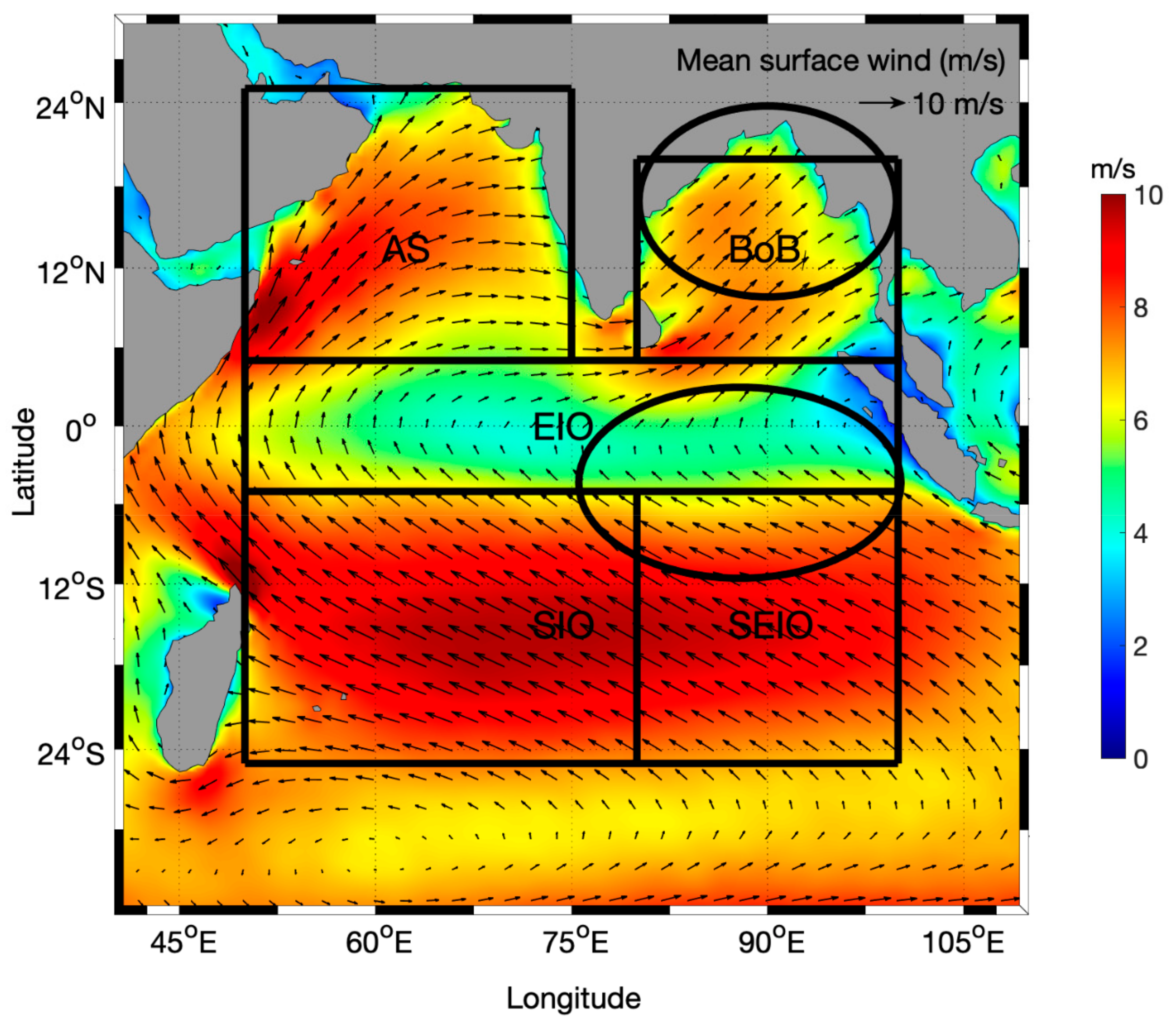
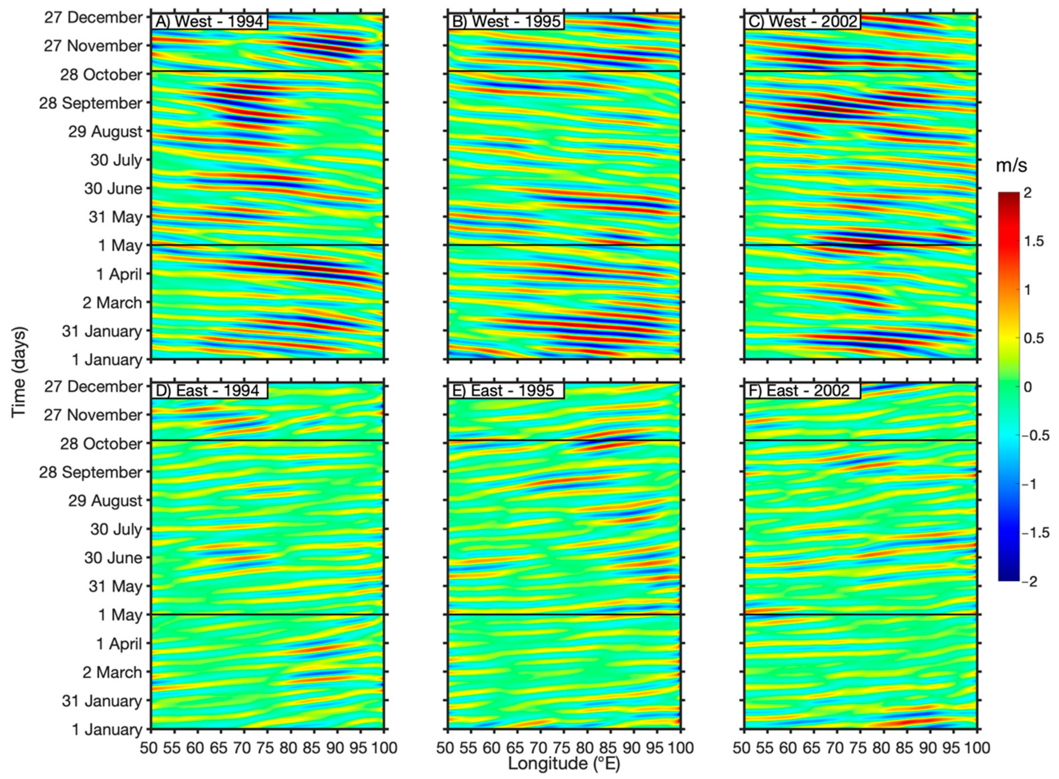
3.1. Regional Comparison of 10–20-Day Signals

During the southwest monsoon, prevailing surface winds over the Indian Ocean are westerly in the north and easterly in the south, with winds largely being southwesterly over India (Figure 1). The strength of these winds varies substantially interannually, which impacts the strength of the monsoon and the rainfall. To determine how the 10–20-day mode in surface wind varies with monsoon strength (meaning the strength for a monsoon season), a strong monsoon (1994), normal monsoon (1995), and weak monsoon (2002) were compared, with monsoon strength determined by the criteria from the Indian Institute of Tropical Meteorology (IITM) [16], where a strong (weak) monsoon is defined as having total rainfall that is 10% above (below) the long-term mean. These years were chosen for this case study based on the IITM climatology and criteria, as 1994 was the last strong monsoon year prior to 2019, 2002 was an anomalously weak year, and 1995 was normal. Impacts of the ENSO or Indian Ocean Dipole (IOD) phase were not considered for this study but warrant future investigation given their impact on equatorial wind stress and Kelvin wave propagation, among other processes.

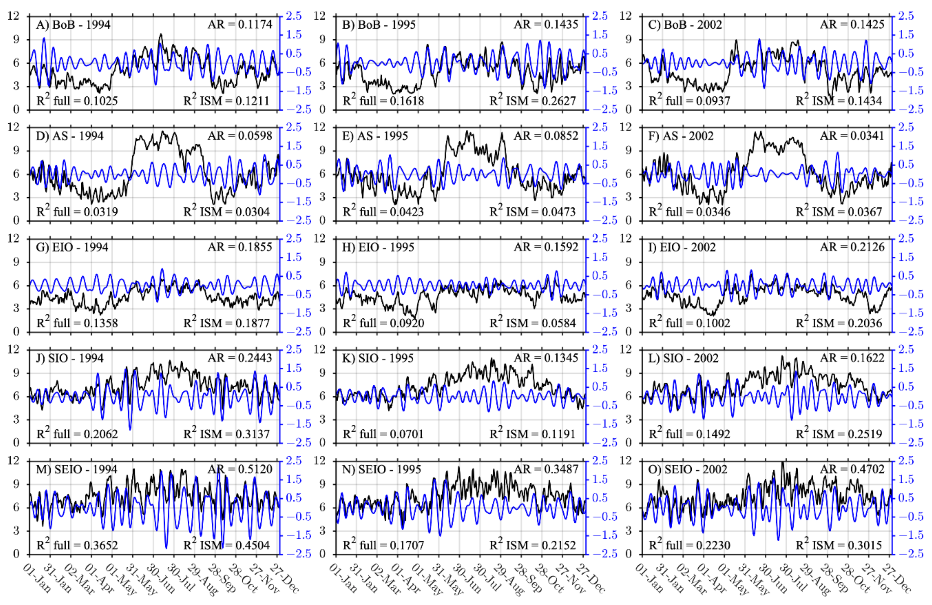
Given that the active (flood) and break (drought) phases of the monsoon associated with the 10–20-day mode are characterized by mesoscale cyclones over the Bay of Bengal, it would be expected that this basin would present the strongest 10–20-day signal of the three basins and that this signal would be most prominent in both strong and weak monsoon years. Comparative analysis of the unfiltered surface wind time series and the bandpass-filtered time series would seem to suggest that this is not necessarily the case (Figure 2). Though the biweekly signal in the Bay can explain up to 26% of surface wind variability during a normal monsoon year (R² = 26%; amplitude ratio = 0.1435; Figure 2B), this variability explained is low during strong (R² = 12%; amplitude ratio = 0.1174; Figure 2A) and weak (R² = 14%; amplitude ratio = 0.1425; Figure 2C) monsoon years and is not the largest amplitude signal in the Indian Ocean as the SIO has a similar amplitude. Previous studies of the 10–20-day mode in the Bay suggested that wind associated with the northernmost cell in the north/central Bay (10–15°N, 85–90°E) were largely responsible for the majority of the oceanic response in the region, particularly regarding upwelling processes in the central Bay, supporting the importance of 10–20-day winds and rain in this region [7], even if it is not the highest amplitude signal. As other atmospheric processes, such as the MJO and tropical cyclones, are extremely active in the Bay and control a larger portion of the precipitation in the basin, it is also unsurprising that the relative amplitude of the signal might be comparatively weak.

While not the basin where the signal is generated, the Arabian Sea is the demise location for many of the mesoscale systems that comprise the 10–20-day mode over India. It is therefore surprising that it has the lowest variability of any region in the greater Indian Ocean, with no significant signals apparent and the amount of variance explained never exceeding 5% (Figure 2D,F) of the variability identified over a year. This is consistent with previous studies of 10–20-day rainfall, which found that the double cell had largely dissipated by the time it reached the Arabian Sea [7,8]. However, the amplitude of the 10–20-day signal is quite substantial during many parts of each of the shown years.

The surface winds in the equatorial Indian Ocean are reasonably well characterized by the 10–20-day mode of variability (Figure 2G–I). Regardless of monsoon strength, the signal remains low amplitude (±1 m/s) with a wide range of variance explained, ranging from 5% to 20%, suggesting that, for this basin, other modes of variability may be more dominant, such as the MJO or Boreal Summer Intraseasonal Oscillation (BSISO) during different times of the year and different monsoon regimes [8,15,17,18,19,20,21,22,23,24,25]. This is reasonably consistent with previous studies, which found that the equatorial Indian Ocean has a low 10–20-day signal, despite being the location of much of the double-cell structure [5], suggesting that monsoon strength in this region is dominated by other processes, such as the equatorially trapped MJO. If the amplitude ratios of the unfiltered and filtered signals are considered, however, it can be seen that they are even higher than those found in the Bay of Bengal, suggesting that, while the wind variability may not be high in the equatorial Indian Ocean, the 10–20-day mode does still play a major role. As the 10–20-day mode only explains roughly 20% of monsoon variability overall [26], amplitude ratios in the equatorial Indian Ocean of 0.1592–0.2126 for surface wind are not unreasonable.

Though the Bay of Bengal and equatorial Indian Ocean are where the majority of precipitation associated with the 10–20-day mode of variability has been noted to take place [2,3,4], it is the southern Indian Ocean and southeastern Indian Ocean that are best described by the 10–20-day mode for winds (Figure 2J–L). The winds in the southern Indian Ocean remain energetic most of the year, though they do experience a slight increase in magnitude during monsoon season. The weak (R² = 25%; amplitude ratio = 0.1622; Figure 2L) and strong (R² = 31%; amplitude ratio = 0.2443; Figure 2J) monsoon years have the highest variability explained. Most notable about the southern Indian Ocean surface winds, however, is not the magnitude but the clearly defined 10–20-day mode of variability apparent in them, even in the unfiltered winds. Of the five regions analyzed, the southeastern Indian Ocean has the highest amplitude 10–20-day bandpass-filtered winds, reflective of the strength of this 10–20-day mode in this region regardless of monsoon regime (Figure 2M–O). The 10–20-day mode is high amplitude during all 3 years analyzed but especially so during the strong monsoon season (R² = 45%; amplitude ratio = 0.5120; Figure 2M). During this strong monsoon, the 10–20-day wind clearly aligns with peaks in the unfiltered winds throughout the season.

These results, while surprising, are critically important to this study and have implications in a much broader context, for modeling and operational studies. Atmospheric circulations that are paired across the equator typically share the upward segment of the vertical circulation. The pair of cells can move zonally with each other. Alternatively, if one cell is stationary, as has been said to be the case [3,4] for the northern cell, then variability in that cell would likely depend on the location of the southern cell, with equatorial convection enhanced when the southern cell is in the same longitudinal position as the northern cell. In Section 3.3, we demonstrate that this second example is the case with the circulation that causes the 10–20-day mode of variability, consistent with the findings of [3,4,8]. The relative dominance of this mode of variability on surface winds in the southern and southeastern Indian Ocean, especially during a strong monsoon season, suggests that any model analysis that does not properly capture or take into account the 10–20-day mode of variability over these regions could be missing up to 31% of surface wind variability in the southern Indian (45% in the southeastern Indian Ocean), as well as inaccurately forecasting the 10–20-day contribution to active and break cycles of the monsoon. Testing this hypothesis requires a weather modeling study, which is outside the scope of this observation-based analysis.

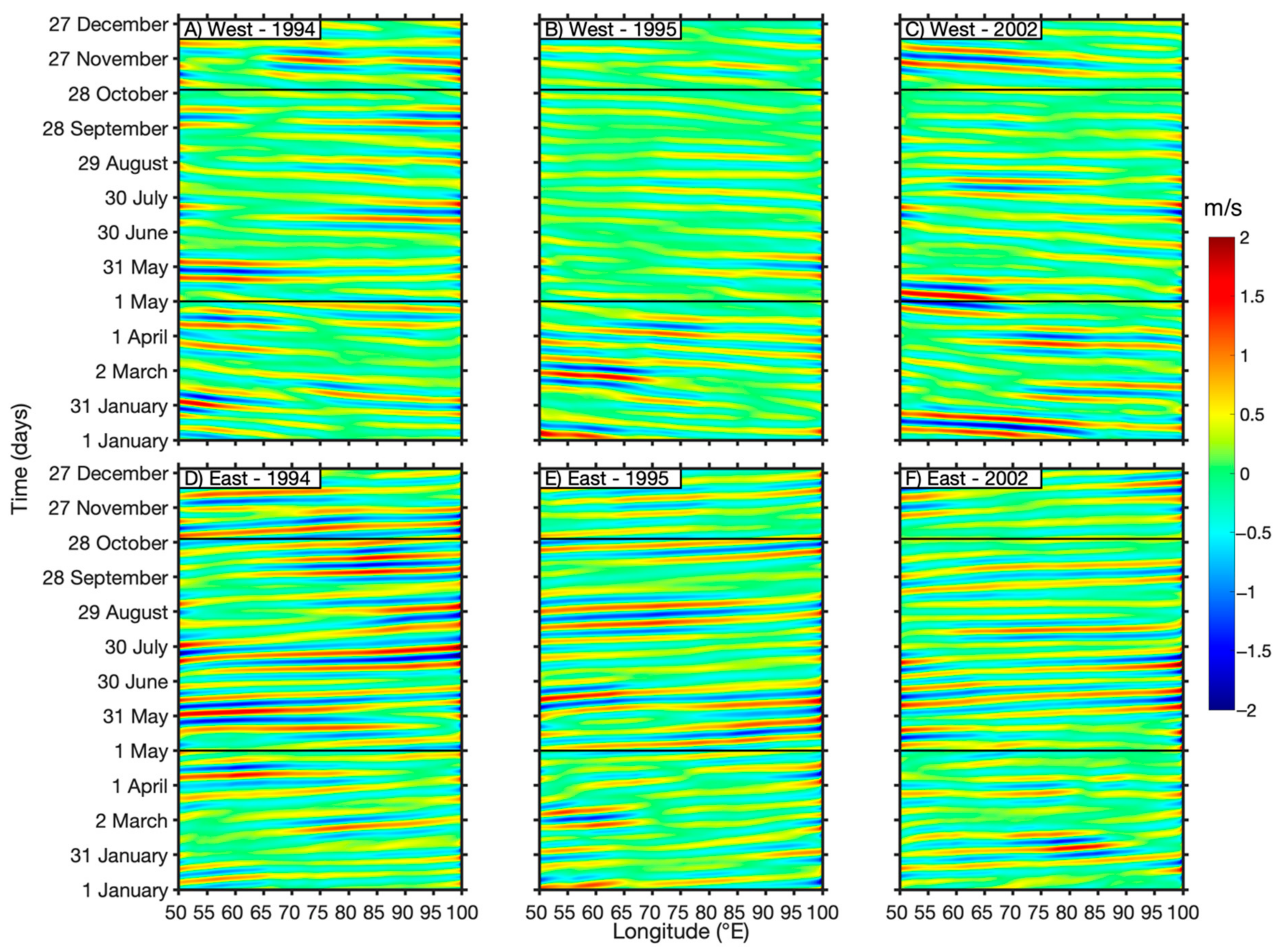
3.2. Signal Propagation in the Southern Indian Ocean

The 10–20-day mode of variability as characterized by rainfall is known to be a westward propagating system of Rossby waves generated by convection in the western Pacific and Bay of Bengal with a meridional double-cell structure that moves northwest over India (Figure 1), with a matched pair of demise regions in the Arabian Sea and southern Indian Ocean [3,4]. In this section, we will explore how well surface winds adhere to this model of signal propagation.

To this end, time–longitude Hovmöller diagrams were 10–20-day bandpass filtered and further directionally filtered with a two-dimensional fast Fourier transform to isolate westward (top panels) and eastward (bottom panels) propagation. The Hovmöller diagrams in the southern Indian Ocean (50–100°E, 5–25°S) for all three monsoon years clearly show the strong zonal 10–20-day signal during all monsoon years (Figure 3). The westward propagation west of 75°E may be due to the double-cell structure and mesocyclones characteristic of this mode as they move to the northwest over India from the Bay of Bengal, though it would not account for the eastward propagation also apparent, particularly in the western half of the ocean. During all three regimes, there is not a clearly defined monsoon season in the western propagation, although the strongest signals occur during this season for the normal and weak monsoon years, especially in the eastern propagating signals. The southeastern Indian Ocean experiences a peak in surface winds during the boreal summer months and a relative decrease in winds during boreal winter, which may be reflective of this seasonality [27].

Given that the 10–20-day mode is a westward propagating system, it is therefore curious that much of the signal propagation west of 75°E in the Indian Ocean would appear to be eastward propagating. It is then proposed that the eastward propagating signal of the 10–20-day mode of variability is associated with reflected westward propagating MRG waves in the ocean, as suggested previously by [8] in relation to the southern cell of the 10–20-day mode, as the magnitude and structure of the signal is not inconsistent with this type of wave. This would seem to be supported by the apparent coupling of eastward and westward propagating signals in the 10–20-day mode, as characterized by [8], who found that patterns of sea level anomalies associated with the southern cell of the double-cell structure are eastward propagating and reflective of an MRG wave [8,28,29].

Another possible explanation, which may not be mutually exclusive, follows the lifecycle of the 10–20-day mode set forth by [5]. In their model for development, the southernmost cell of the double-cell structure originates as a convective anomaly in the western Indian Ocean [5]. This convective anomaly then propagates east until it couples with the northern cell and moves westward. As the Arabian Sea is the demise location for many of these double-cell events, that would account for the westward propagation that often follows an eastward event. It is therefore plausible that the east/west pairings of signals shown here is a combination of multiple signals, both in the form of MRG waves and these convective anomalies moving back and forth across India.

To further assess the viability of this MRG wave theory, Hovmöller diagrams of the meridional component of the wind were created in the equatorial Indian Ocean (Figure 4), the zonal propagation of which have been shown to be characteristic of MRG waves [29]. The westward propagation in equatorial meridional winds has higher amplitude than the eastward propagation across all three monsoon regimes, although eastward propagation is still apparent, with high-amplitude eastward propagation most often being coupled with strong westward signals. These results strongly confirm the presence of MRG waves associated with the 10–20-day mode, but given the infrequency of strong eastward signals, it is likely that any reflection as previously mentioned is rare and another mechanism is chiefly responsible for the strong eastward propagation observed in the southern Indian Ocean (Figure 3). Further research is necessary to identify the precise source of these eastward signals, and while the identified explanations are two possible mechanisms that may explain some of the variability, a more thorough study beyond the scope of this case study is required.

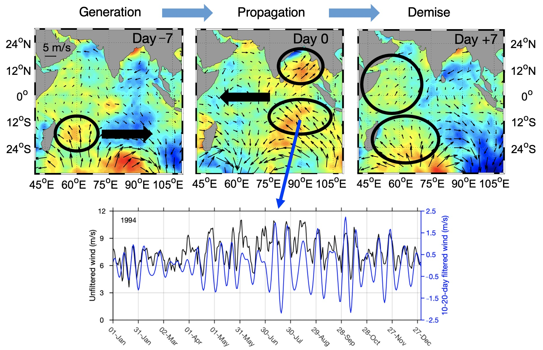
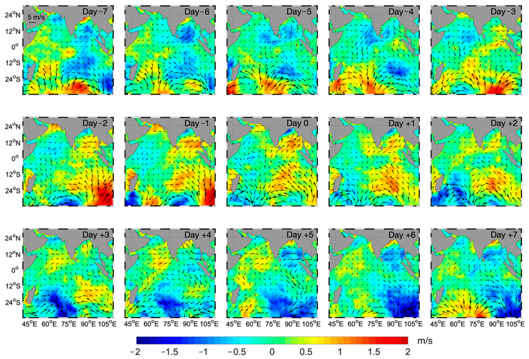
3.3. Composite Analysis

Given the results of previous sections, composites were constructed based on a time series of the southeastern Indian Ocean (80–100°E, 5–25°S), which was found to have the highest fraction of variance explained by the 10–20-day mode during the southwest monsoon season (R² = 45%) in the region (Figure 2). It was therefore anticipated that the majority of activity seen in the composites would occur in the southeastern Indian Ocean. In contrast, previous studies [2,4,30] suggest that most variability would occur in the Bay of Bengal region given that this is the location of the northern cell. In viewing the composite breakdown of the 10–20-day mode identified (Section 2.2), the signal that is most apparent is in the southeastern Indian Ocean, but there are also prominent signals in the Bay of Bengal and Arabian Sea (Figure 5). We will show that the variability in the northern cell is in phase with the location of the southern cell.

Little appears to change between Day −7 and Day −5. During these three days, there is a modest positive wind anomaly in the southern Indian Ocean centered around 60°E off the coast of Madagascar and a negative wind anomaly between the equator and 5°N. On Day −4, however, there is a substantial increase in the positive wind anomalies at 15°S between 55°E and 85°E and in the eastern equatorial Indian Ocean. On Day −3, a positive wind anomaly emerges in the Bay of Bengal, which likely accompanies the arrival of the northern cell into the Bay. Between Days −3 and Day −1, both of these wind anomalies continue to grow, becoming more clearly defined, and with the southern cell shifting eastward several degrees. At Day 0—the peak of the composite curve—the positive anomalies have their greatest values. After Day 0, the wind anomalies begin to rapidly weaken. By Day +4, the positive anomalies have lost most of their defined structure and the energy begins to disperse westward towards Madagascar around the Mascarene High for the southern cell and the Arabian Sea for the northern cell. This southern progression of phases has the overall effect of having a large positive wind anomaly at 15°S slosh back and forth across the basin, taking roughly seven days to cross each way and reaching its peak magnitude in the eastern portion of the basin. In contrast, the northern cell is largely confined to the Bay of Bengal and Arabian Sea, as seen in previous studies [2,3,4]. This northern cell drives upwelling in the central Bay, leading to a salinification and net cooling of the Bay by Day +4 [7]. However, the variability in the northern cell is linked to the position of the southern cell, with the greatest strength when the southern cell enhances equatorial convection in the northern cell.

The emergence of the signal at Day −4 is likely due to convective anomalies emerging out of the western Pacific that trigger a Rossby wave response in both hemispheres [5,6,7,8]. Given the longitudes at which it forms and then reverses direction, however, it would seem to almost perfectly follow the path of the southernmost cell of the convective double-cell structure characteristic of this mode [3,5,6,7,8]. The southernmost cell has been shown to be triggered around 5°S by an MRG wave, as seen in the propagation of sea level anomalies in the eastern equatorial Indian Ocean [8]. The precipitation associated with the vortex and the convective cell are not perfectly aligned, with the convection having a greater lateral distribution which stretches much deeper into the southern hemisphere [4,5]. This would suggest that the observed wind anomaly is reflective of the convective cell which is centered farther south than the precipitation associated with the vortex [3,4,5,8].

Though the complete convective double-cell structure itself is not as readily apparent in surface winds as it is in OLR or precipitation from the Tropical Rainfall Measurement Mission (TRMM), it is suggested by the positive wind anomalies, which follow a similar pattern to the OLR anomalies and precipitation of past studies [4,5,7,8]. The filtered surface wind anomalies are more fluid and encompass a larger area than the OLR anomalies. This is likely due to the nature of surface winds compared to precipitation or OLR, namely that OLR and precipitation have distinct edges that define them from the clearer air around them, whereas surface winds gridded on a 25 km map lack this definition. While OLR and precipitation are associated with patterns of pressure, surface winds instead follow the pressure gradient, which results in the observed differences seen between the distribution of these variables. OLR anomalies are not entirely consistent in past studies with regards to the location of the northern cell or anomalies to the direct east and west of India, but both patterns are reflected in the filtered surface winds, suggesting that different methods of composite creation may highlight local centers of convection or vorticity, both of which are important for our understanding of the dynamics associated with this mode. The discrepancies between all three studies can be largely attributed to data used and the manner in which the composites were created [4,5,7,8]. Additionally, OLR anomalies can be seen over land, whereas CCMP surface winds cannot, and thus the seemingly isolated patterns on either side of India may be more reflective of a greater anomaly encompassing most of the area, such as the northernmost cell (Figure 1).

The increased activity in the Arabian Sea, particularly after Day +1, is likely reflective of a dynamic connection to the formation and dissipation of the southern cell and its associated energy. As winds in the Arabian Sea peak in response to the winds in the southern cell circulation decreasing, it is possible that the energy dissipated by the demise of the southern cell is transferred to the Arabian Sea, causing this increase in activity. Previous studies have shown consistent OLR and precipitation anomalies over the Arabian Sea throughout, so it is likely that the consistent winds over the Arabian Sea seen in our composites are, at least in part, a product of the weather patterns responsible for the precipitation and OLR in this region (Figure 5) [5].

4. Discussion

The results of our composite analysis suggest that the southernmost cell of the convective double-cell structure associated with the 10–20-day mode in the Indian Ocean is not confined to the equator but has a mode in surface wind that is centered on 15°S and forms east of Madagascar around the Mascarene High, propagates eastward across the basin to 90°E, and then reflects back as an MRG wave, propagating westward across the basin before the energy disperses east of Madagascar, largely traveling up the Somali coast into the Arabian Sea. This mechanism would explain the east and westward propagating signals seen in Figure 3 and Figure 4 and the transfer of energy between the southern cell and the Arabian Sea seen in Figure 5, as well as provide a plausible connection between the northern and southern halves of the greater Indian Ocean basin. This theory would also support the double-cell structure observed and characterized by past studies, extending it further into the southern hemisphere and to include surface winds [4,5,8,28,29].

Although there has not, to the authors’ knowledge, been extensive research into the 10–20-day mode in the southern Indian Ocean, several studies have shown there to be a significant connection between MJO activity and the Mascarene High and Seychelles–Chagos thermocline ridge [31,32,33,34,35]. The buildup of near-surface heat due to barrier layer formation along the Seychelles–Chagos thermocline ridge creates the conditions necessary for MJO genesis, particularly between August and December [33]. Further research into the coupling between MJO activity and the Seychelles–Chagos thermocline found that MJO air–sea fluxes were responsible for anomalous cooling observed in the region during the 2002 monsoon season [34]. An analysis of surface wind variability in the thermocline region also found that there was a possibly strong connection between sea surface temperatures during boreal winter and southwest monsoon strength in the following season, citing upwelling and downwelling processes associated with Rossby wave propagation as a primary control on the observed variability [32]. These studies would seem to support our findings, that surface wind variability in the southern Indian Ocean around the Mascarene High associated with a convectively coupled Rossby wave feeds back into the double-cell structure of the 10–20-day mode. Furthermore, it provides a mechanism for MJO and 10–20-day co-occurrence and cascading energy, which would explain the frequency of event co-occurrence in recent monsoon years [26].

5. Conclusions

The 10–20-day mode of variability in the Indian Ocean is one of the most prominent intraseasonal oscillations related to the southwest monsoon and is one of the primary controls on the active and break cycles of precipitation over India. Statistical analysis showed that the 10–20-day mode could explain less than 20% of the total surface wind variability in the equatorial Indian Ocean and Arabian Sea regardless of monsoon strength, suggesting that it is not the 10–20-day mode but rather the 15–30-day or 30–90-day modes that most likely dominate wind speed variability in this region. The Bay of Bengal presents a stronger 10–20-day signal, although at no point does the 10–20-day mode explain more than 26% of the surface wind variance explained in this region. That being said, 10–20-day surface wind in the Bay of Bengal has been shown to modulate coastal Kelvin wave propagation in the Bay [8] and drive upwelling in the central Bay [7], and so there can still be significant impacts by 10–20-day wind, even if it is not the dominant signal. The southern Indian Ocean showed the most significant seasonal variability, with 12% and 25% of surface wind variance being explained by the 10–20-day mode during normal (1995) and weak (2002) monsoon years, respectively. By contrast, more than 31% of the surface wind variance can be explained by the 10–20-day mode in this region during a strong monsoon year (1994), with this number increasing to 45% when only the southeastern Indian Ocean is considered, suggesting a relative dominance of the 10–20-day mode of variability in the southern Indian Ocean, especially during strong monsoon years.

Hovmöller diagrams show that the majority of the activity in the 10–20-day mode occurs west of 75°E, with further analysis suggesting that there is a reflection around 60°E between eastward and westward propagating signals. As the western Indian Ocean is the genesis region for the southernmost cell of the double cell, this presents a possible source of the eastward propagation, with the coupling with the northernmost cell and the ensuing demise of the system resulting in the observed westward propagation. This further suggests possible connections to other eastward propagating systems in the Indian Ocean that occur on intraseasonal timescales, such as the MJO and Kelvin waves.

Through these composites, a large positive wind anomaly was discovered to be in the southern Indian Ocean, centered on 15°S and forming off the eastern coast of Madagascar around 60°E and the Mascarene High. This wind anomaly moves eastward until it reaches 90°E, at which point it changes direction and moves westward, dissipating near Madagascar and its genesis region. This pattern was already noted in the Hovmöller diagram analysis and bears a striking resemblance to the activity of the southernmost cell of the double-cell structure. We therefore propose that this positive wind anomaly is a feature of the southernmost cell of the convective double-cell structure in the southern Indian Ocean, as supported by OLR, TRMM precipitation anomalies, and sea level anomalies, noted by previous studies [4,5,8]. We hypothesize that interaction of the northern cell with the southern cell organizes physically important variability of the northern cell.

In the composite fields, it is apparent as well that there is a connection to convection in the Southern Ocean. This convection ties into the southernmost cell of the convective cell structure and likely contributes to the overall variability seen on this time scale. As it is austral winter in the southern hemisphere during this Indian summer monsoon season, it is possible that mid-latitude cyclonic activity in the Southern Ocean contributes to the 10–20-day mode seen in the Indian Ocean. If found to be true in further research, this would connect the Southern Ocean to the Indian Ocean and Bay of Bengal. Further research, however, will need to further investigate this possible connection and its consequences.

References

1. Madden, R.A.; Julian, P.R. Detection of a 40–50 Day Oscillation in the Zonal Wind in the Tropical Pacific. J. Atmos. Sci. 1971, 28, 702–708. [Google Scholar] [CrossRef]
2. Krishnamurti, T.N.; Ardanuy, P. The 10 to 20-day Westward Propagating Mode and “Breaks in the Monsoons”. Tellus 1980, 32, 15–26. [Google Scholar] [CrossRef] [Green Version]
3. Chen, T.-C.; Chen, J.-M. The 10–20-Day Mode of the 1979 Indian Monsoon: Its Relation with the Time Variation of Monsoon Rainfall. Mon. Weather Rev. 1993, 121, 2465–2485. [Google Scholar] [CrossRef]
4. Chatterjee, P.; Goswami, B.N. Structure, Genesis and Scale Selection of the Tropical Quasi-Biweekly Mode. Q. J. R. Meteorol. Soc. 2004, 130, 1171–1194. [Google Scholar] [CrossRef] [Green Version]
5. Kikuchi, K.; Wang, B. Global Perspective of the Quasi-Biweekly Oscillation. J. Clim. 2009, 22, 1340–1359. [Google Scholar] [CrossRef]
6. Ortega, S.; Webster, P.J.; Toma, V.; Chang, H.R. Quasi-Biweekly Oscillations of the South Asian Monsoon and Its Co-Evolution in the Upper and Lower Troposphere. Clim. Dyn. 2017, 49, 3159–3174. [Google Scholar] [CrossRef]
7. Roman-Stork, H.L.; Subrahmanyam, B.; Murty, V.S.N. Quasi-Biweekly Oscillations in the Bay of Bengal in Observations and Model Simulations. Deep-Sea Res. Part II Top. Stud. Oceanogr. 2019, 168, 104609. [Google Scholar] [CrossRef]
8. Roman-Stork, H.L.; Subrahmanyam, B.; Trott, C.B. Monitoring Intraseasonal Oscillations in the Indian Ocean Using Satellite Observations. J. Geophys. Res. Ocean. 2020, 125, e2019JC015891. [Google Scholar] [CrossRef]
9. Goswami, B.N.; Sengupta, D.; Suresh Kumar, G. Intraseasonal Oscillations and Interannual Variability of Surface Winds over the Indian Monsoon Region. Proc. Indian Acad. Sci.-Earth Planet. Sci. 1998, 1–7, 45–64. [Google Scholar] [CrossRef] [Green Version]
10. Atlas, R.; Oceanic, N.; Hoffman, R.N.; Leidner, S.M. Development of a New Cross-Calibrated, Multi-Platform (CCMP) Ocean Surface Wind Product. In Proceedings of the AMS 13th Conference Integrated Observing and Assimilation Systems for Atmosphere, Oceans, and Land Surface (IOAS-AOLS), College Park, MD, USA, 10 January 2009. [Google Scholar]
11. Atlas, R.; Hoffman, R.N.; Ardizzone, J.; Leidner, S.M.; Jusem, J.C.; Smith, D.K.; Gombos, D. A Cross-Calibrated, Multiplatform Ocean Surface Wind Velocity Product for Meteorological and Oceanographic Applications. Bull. Am. Meteorol. Soc. 2011, 92, 157–174. [Google Scholar] [CrossRef]
12. Hoffman, R.N.; Leidner, S.M.; Henderson, J.M.; Atlas, R.; Ardizzone, J.V.; Bloom, S.C. A Two-Dimensional Variational Analysis Method for NSCAT Ambiguity Removal: Methodology, Sensitivity, and Tuning. J. Atmos. Ocean. Technol. 2003, 20, 585–605. [Google Scholar] [CrossRef]
13. Huang, N.E.; Wu, Z. A Review on Hilbert-Huang Transform: Method and Its Applications. Rev. Geophys. 2008, 46, 1–23. [Google Scholar] [CrossRef] [Green Version]
14. Wu, Z.; Huang, N.E. Ensemble Empirical Mode Decomposition: A Noise-Assisted Data Analysis Method. Adv. Adapt. Data Anal. 2009, 1, 1–41. [Google Scholar] [CrossRef]
15. Krishnamurti, T.N.; Jana, S.; Krishnamurti, R.; Kumar, V.; Deepa, R.; Papa, F.; Bourassa, M.A.; Ali, M.M. Monsoonal Intraseasonal Oscillations in the Ocean Heat Content over the Surface Layers of the Bay of Bengal. J. Mar. Syst. 2017, 167, 19–32. [Google Scholar] [CrossRef]
16. Zheng, Y.; Ali, M.M.; Bourassa, M.A. Contribution of Monthly and Regional Rainfall to the Strength of Indian Summer Monsoon. Mon. Weather Rev. 2016, 144, 3037–3055. [Google Scholar] [CrossRef]
17. Wang, B.; Xie, X. A Model for the Boreal Summer Intraseasonal Oscillation. J. Atmos. Sci. 1997, 54, 72–86. [Google Scholar] [CrossRef] [Green Version]
18. Lawrence, D.M.; Webster, P.J. The Boreal Summer Intraseasonal Oscillation: Relationship between Northward and Eastward Movement of Convection. J. Atmos. Sci. 2002, 59, 1593–1606. [Google Scholar] [CrossRef]
19. Ajayamohan, R.S.; Rao, S.A.; Yamagata, T. Influence of Indian Ocean Dipole on Poleward Propagation of Boreal Summer Intraseasonal Oscillations. J. Clim. 2008, 21, 5437–5454. [Google Scholar] [CrossRef]
20. Straub, K.H.; Kiladis, G.N. Interactions between the Boreal Summer Intraseasonal Oscillation and Higher-Frequency Tropical Wave Activity. Mon. Weather Rev. 2003, 131, 945–960. [Google Scholar] [CrossRef]
21. Ajayamohan, R.S.; Annamalai, H.; Luo, J.J.; Hafner, J.; Yamagata, T. Poleward Propagation of Boreal Summer Intraseasonal Oscillations in a Coupled Model: Role of Internal Processes. Clim. Dyn. 2011, 37, 851–867. [Google Scholar] [CrossRef]
22. Zhang, C. Madden-Julian Oscillation. Rev. Geophys. 2005, 43, 2004RG000158. [Google Scholar] [CrossRef] [Green Version]
23. Matthews, A.J. Primary and Successive Events in the Madden-Julian Oscillation. Q. J. R. Meteorol. Soc. A J. Atmos. Sci. Appl. Meteorol. Phys. Oceanogr. 2008, 134, 439–453. [Google Scholar] [CrossRef] [Green Version]
24. Bhatla, R.; Singh, M.; Pattanaik, D.R. Impact of Madden-Julian Oscillation on Onset of Summer Monsoon over India. Theor. Appl. Climatol. 2017, 128, 381–391. [Google Scholar] [CrossRef]
25. Shoup, C.G.; Roman-Stork, H.L.; Subrahmanyam, B. Analysis of Coupled Oceanic and Atmospheric Preconditioning for Primary Madden-Julian Oscillation Events Across ENSO Phases. J. Geophys. Res. Ocean. 2020, 125, 1–20. [Google Scholar] [CrossRef]
26. Subrahmanyam, B.; Roman-Stork, H.L.; Murty, V.S.N. Response of the Bay of Bengal to 3-7-Day Synoptic Oscillations during the Southwest Monsoon of 2019. J. Geophys. Res. Ocean. 2020, 125, 1–28. [Google Scholar] [CrossRef]
27. Loschnigg, J.; Webster, P.J. A Coupled Ocean-Atmosphere System of SST Modulation for the Indian Ocean. J. Clim. 2000, 13, 3342–3360. [Google Scholar] [CrossRef]
28. Chatterjee, A.; Shankar, D.; McCreary, J.P.; Vinayachandran, P.N. Yanai Waves in the Western Equatorial Indian Ocean. J. Geophys. Res. Ocean. 2013, 118, 1556–1570. [Google Scholar] [CrossRef]
29. Sengupta, D.; Senan, R.; Murty, V.S.N.; Fernando, V. A Biweekly Mode in the Equatorial Indian Ocean. J. Geophys. Res. C Ocean. 2004, 109, 1–12. [Google Scholar] [CrossRef]
30. Murakami, M. Analysis of Summer Monsoon Fluctuations over India. J. Meteorol. Soc. Jpn. 1976, 54, 15–31. [Google Scholar] [CrossRef] [Green Version]
31. Hermes, J.C.; Reason, C.J.C. Annual Cycle of the South Indian Ocean (Seychelles-Chagos) Thermocline Ridge in a Regional Ocean Model. J. Geophys. Res. Ocean. 2008, 113, e2007JC004363. [Google Scholar] [CrossRef]
32. Hermes, J.C.; Reason, C.J.C. The Sensitivity of the Seychelles-Chagos Thermocline Ridge to Large-Scale Wind Anomalies. ICES J. Mar. Sci. 2009, 66, 1455–1466. [Google Scholar] [CrossRef] [Green Version]
33. D’Addezio, J.M.; Subrahmanyam, B. Evidence of Organized Intraseasonal Convection Linked to Ocean Dynamics in the Seychelles–Chagos Thermocline Ridge. Clim. Dyn. 2018, 51, 3405–3420. [Google Scholar] [CrossRef]
34. Jayakumar, A.; Gnanaseelan, C. Anomalous Intraseasonal Events in the Thermocline Ridge Region of Southern Tropical Indian Ocean and Their Regional Impacts. J. Geophys. Res. Ocean. 2012, 117, e2011JC007357. [Google Scholar] [CrossRef] [Green Version]
35. Jayakumar, A.; Vialard, J.; Lengaigne, M.; Gnanaseelan, C.; McCreary, J.P.; Kumar, B.P. Processes Controlling the Surface Temperature Signature of the Madden-Julian Oscillation in the Thermocline Ridge of the Indian Ocean. Clim. Dyn. 2011, 37, 2217–2234. [Google Scholar] [CrossRef] [Green Version]
Figure 1. Mean May–October surface wind magnitude over the Indian Ocean (shaded; m/s) overlaid with wind vectors (vectors; m/s). Boxes designate regions used for comparative time series: the Arabian Sea (AS; 50–75°E, 5–25°N), Bay of Bengal (BoB; 80–100°E, 5–20°N), equatorial Indian Ocean (EIO; 50–100°E, 5°S–5°N), southern Indian Ocean (SIO; 50–100°E, 5–25°S), and southeastern Indian Ocean (SEIO; 80–100°E, 5–25°S). Black circles indicate the general locations of the northern (top) and southern (bottom) cells in the 10–20-day double-cell structure.
Remotesensing 14 03419 g001
Figure 2. Unfiltered box averaged surface wind magnitude (black; m/s) over the Bay of Bengal (BoB; (AC)), Arabian Sea (AS; (DF)), equatorial Indian Ocean (EIO; (GI)), southern Indian Ocean (SIO; (JL)), and southeastern Indian Ocean (SEIO; (MO)) overlaid with 10–20-day bandpass-filtered time series of the same regions (blue; m/s) during 1994 (strong; left), 1995 (normal; middle), and 2002 (weak; right). R2 values describe the variance explained by the 10–20-day mode for the full year (R2 full) and during May–October (R2 ISM). Amplitude ratio (AR) values are displayed in the upper left corner of each subplot and represent the ratio between the actual filtered portion of the signal compared to the overall signal for a given region.
Remotesensing 14 03419 g002
Figure 3. Time–longitude plots of 10–20-day bandpass-filtered surface wind magnitude (shaded; m/s) in the southern Indian Ocean during a strong (A,D), normal (B,E), and weak (C,F) monsoon season that is filtered for westward (AC) and eastward (DF) propagation. A positive slope indicates that a feature is moving eastward as time progresses, and a negative slope means that a feature is propagating westward. The extended southwest monsoon season (May–October) is indicated by black lines on the plot.
Remotesensing 14 03419 g003
Figure 4. Time–longitude plots of 10–20-day bandpass-filtered meridional surface wind (shaded; m/s) in the equatorial Indian Ocean during a strong (A,D), normal (B,E), and weak (C,F) monsoon season that is filtered for westward (AC) and eastward (DF) propagation. The extended southwest monsoon season (May–October) is indicated by black lines on the plot.
Remotesensing 14 03419 g004
Figure 5. Time-lag composites of surface wind magnitude (shaded; m/s) in the Indian Ocean based on a 10–20-day bandpass-filtered time series in the southeastern Indian Ocean, overlaid with surface wind vectors.
Remotesensing 14 03419 g005
Publisher’s Note: MDPI stays neutral with regard to jurisdictional claims in published maps and institutional affiliations.