Article

Estimating Community-Level Plant Functional Traits in a Species-Rich Alpine Meadow Using UAV Image Spectroscopy

1
Institute of Ecology, College of Urban and Environmental Sciences and Key Laboratory for Earth Surface Processes of the Ministry of Education, Peking University, Beijing 100871, China
2
Faculty of Geo-Information Science and Earth Observation (ITC), University of Twente, P.O. Box 217, 7500 AE Enschede, The Netherlands
3
Key Laboratory of Adaptation and Evolution of Plateau Biota and Qinghai Provincial Key Laboratory of Restoration Ecology of Cold Area, Northwest Institute of Plateau Biology, Chinese Academy of Sciences, Xining 810008, China
*
Author to whom correspondence should be addressed.
Remote Sens. 2022, 14(14), 3399; https://doi.org/10.3390/rs14143399
Submission received: 24 May 2022 / Revised: 4 July 2022 / Accepted: 11 July 2022 / Published: 15 July 2022
(This article belongs to the Special Issue Remote Sensing of Vegetation Function and Traits)

Abstract

:
Plant functional traits at the community level (plant community traits hereafter) are commonly used in trait-based ecology for the study of vegetation–environment relationships. Previous studies have shown that a variety of plant functional traits at the species or community level can be successfully retrieved by airborne or spaceborne imaging spectrometer in homogeneous, species-poor ecosystems. However, findings from these studies may not apply to heterogeneous, species-rich ecosystems. Here, we aim to determine whether unmanned aerial vehicle (UAV)-based hyperspectral imaging could adequately estimate plant community traits in a species-rich alpine meadow ecosystem on the Qinghai–Tibet Plateau. To achieve this, we compared the performance of four non-parametric regression models, i.e., partial least square regression (PLSR), the generic algorithm integrated with the PLSR (GA-PLSR), random forest (RF) and extreme gradient boosting (XGBoost) for the retrieval of 10 plant community traits using visible and near-infrared (450–950 nm) UAV hyperspectral imaging. Our results show that chlorophyll a, chlorophyll b, carotenoid content, starch content, specific leaf area and leaf thickness were estimated with good accuracies, with the highest R2 values between 0.64 (nRMSE = 0.16) and 0.83 (nRMSE = 0.11). Meanwhile, the estimation accuracies for nitrogen content, phosphorus content, plant height and leaf dry matter content were relatively low, with the highest R2 varying from 0.3 (nRMSE = 0.24) to 0.54 (nRMSE = 0.20). Among the four tested algorithms, the GA-PLSR produced the highest accuracy, followed by PLSR and XGBoost, and RF showed the poorest performance. Overall, our study demonstrates that UAV-based visible and near-infrared hyperspectral imaging has the potential to accurately estimate multiple plant community traits for the natural grassland ecosystem at a fine scale.

1. Introduction

Plant functional traits may directly or indirectly affect plant fitness by influencing individuals’ growth, reproduction and survival [1]. They reflect the morphological, physiological or phenological responses of species to the environment and serve as proxies for life strategies [2,3,4]. However, plant species primarily represent and survive as part of a plant community instead of as separate species or individuals. Therefore, the variation in traits among species cannot represent the characteristics of plant communities or vegetation, nor the ecological processes at the ecosystem level [5,6].
Plant communities are composed of sets of species with various abundances and maintain a dynamic balance through interactions between species [7]. Therefore, plant functional traits at the community level (plant community traits hereafter) include information not only on plant functional traits but also on species composition. Plant community traits offer a trait-based approach to address several key questions related to plant community assembling and productivity regulation [8,9] and will assist in exploring how vegetation responds to climate change [10].
The community-weighted mean (CWM) trait, which aggregates plant functional traits at the community level using the weighted-mean approach, is a commonly used indicator for the study of vegetation–environment relationships [7]. The CWM trait is typically calculated as the mean of plant functional trait values at the species level weighted by the relative abundance of taxa [5]. However, measuring CWM traits through field surveys is time-consuming and labour-intensive, while using trait data from published databases is hindered by differences in sampling and measurement criteria and usually ignores intraspecific variation of traits [11]. Moreover, functional traits derived from discrete sites could hardly reflect the continuous spatial change in vegetation characteristics [12]. Hence, an alternative approach to collecting trait information at the community level covering variations within and between species is of great significance [13].
Remote sensing has the potential to provide a spatially continuous representation of plant functional traits and intraspecific variations [14,15]. Previous studies have shown that a variety of plant functional traits at the species or community level in forest ecosystems can be successfully retrieved by airborne or spaceborne imaging spectrometer [16,17]. As to grassland ecosystems, although a few studies have attempted to quantify trait variations at the community level, they are either limited to a relatively homogeneous condition with few co-existing species [18], dependent on a well-managed experimental platform and observed datasets [19] or focus only on limited plant traits [20]. The conclusions drawn from these studies may not apply to heterogeneous and species-rich grasslands in natural conditions [21].
The unmanned aerial vehicle (UAV) platform can be operated flexibly according to weather and field conditions, so it has become increasingly used in ecological research [22,23]. UAV-based imaging spectroscopy is a relatively new remote sensing technology with significant benefits for high-resolution remote sensing applications, making it possible to study trait variations at the community level at a fine scale [24]. Moreover, UAV-based imaging spectroscopy could offer a link between field investigation and satellite observation, which may support the estimation of plant functional traits at the community level on a broader spatial scale [25]. However, despite the potential of UAV-based imaging spectroscopy, little research has been performed on the estimation of plant community traits directly from UAV hyperspectral imagery, particularly in heterogeneous natural grasslands. Thus, in this paper, we aim to determine whether UAV-based hyperspectral imaging could adequately estimate plant community traits in a species-rich alpine meadow. Specifically, we set out to assess the performance of four non-parametric regression models for retrieving 10 plant community traits from visible and near-infrared (450–950 nm) UAV hyperspectral imagery.

2. Materials and Methods
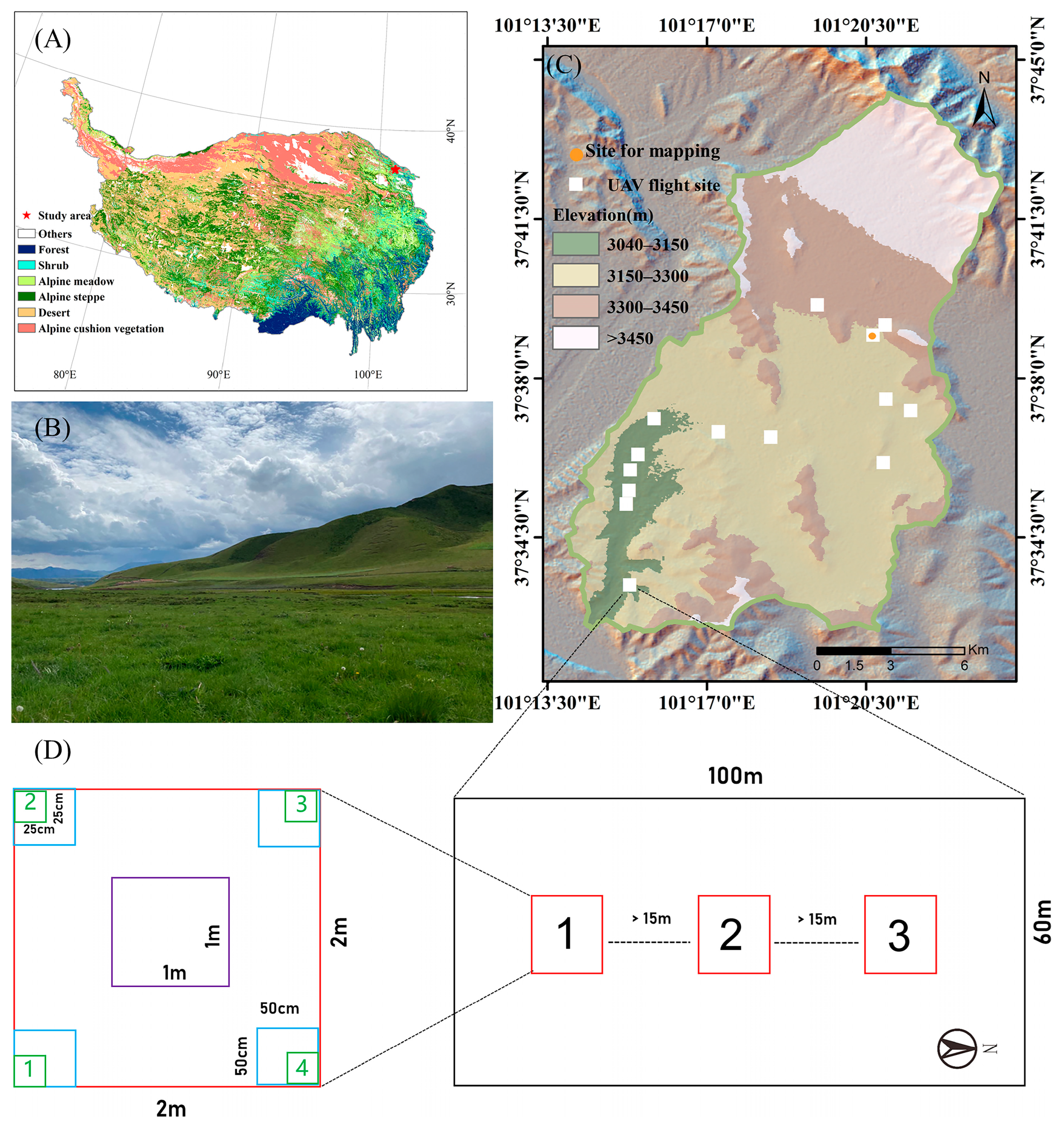
2.1. Study Area

Our study is within a river basin located in the northeastern Qinghai– Tibet Plateau in Qinghai Province, China. The basin covers an area of approximately 244.8 km2 with an average elevation of 3385 m.a.s.l. (Figure 1). This area is characterised by a continental monsoon climate with a mean annual temperature of –1.1 °C and a mean annual precipitation of 485 mm. Around 80% of the precipitation falls in the growing season from mid-April to mid-October. The dominant vegetation communities are alpine meadows and alpine shrubs. These communities are very rich in plant species, ranging from 30 to 50 per square meter [26].

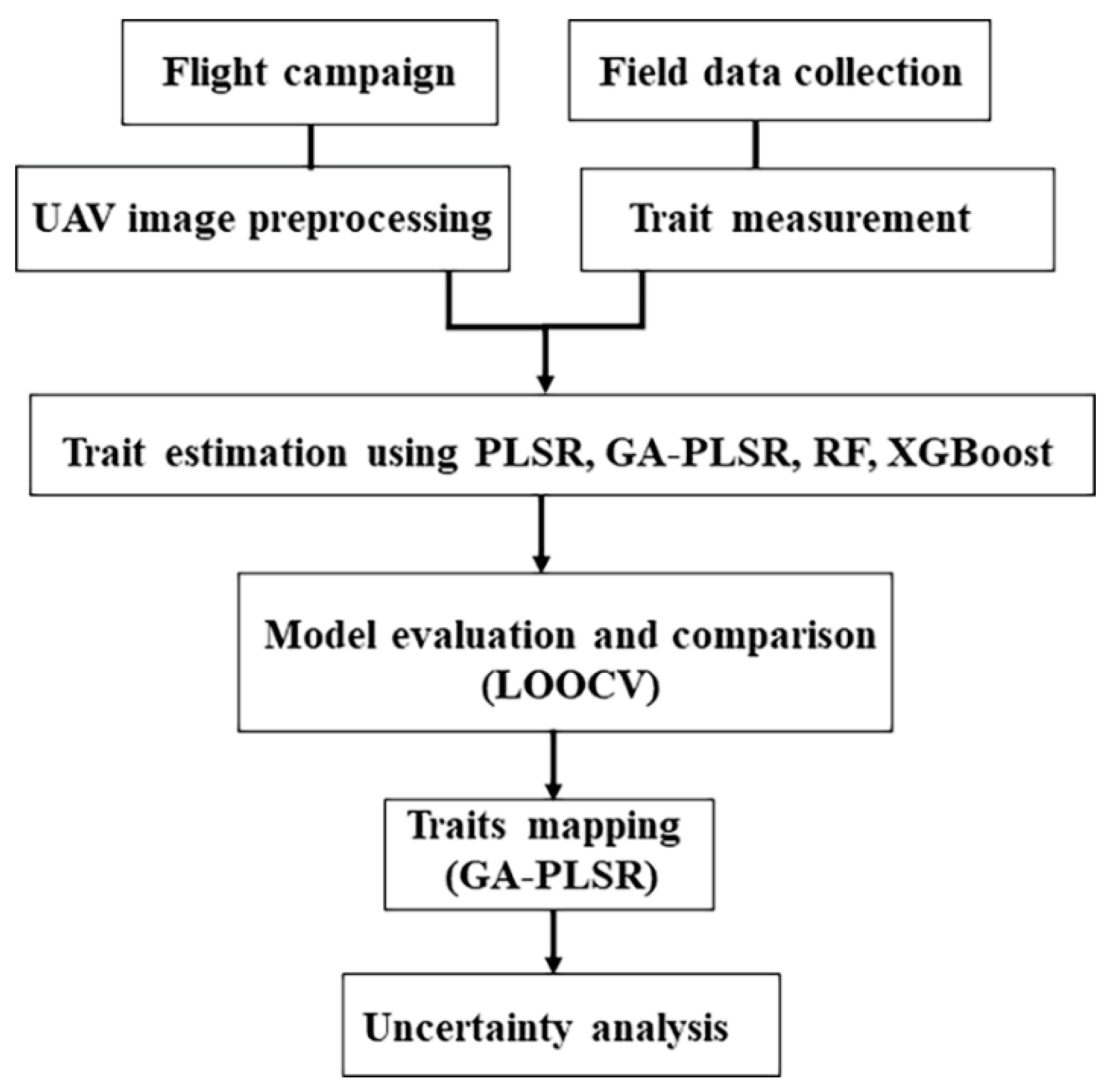
2.2. Hyperspectral Data Collection and Pre-Processing

In this study, we determined 20 survey sites according to the altitude gradients, with the altitude ranging from 3040 to 3450 m. Each survey site was 100 m × 60 m in size. UAV flight campaigns were conducted between 10 and 26 August 2021 during the growing season of the meadow. At each survey site, we collected the hyperspectral data by a Cubert UHD185 Firefly spectrometer (UHD185) equipped on a hexacopter UAV (DJI M600 PRO). DJI M600 PRO was equipped with the A3 Pro flight controller including three Inertial Measurement Units (IMU) and three Global Navigation Satellite System (GNSS) units. The UHD185 comprises 125 spectral channels and spans the spectral range from 450 to 950 nm at a 4-nm sampling interval, and the spectral resolution is 8 nm. One panchromatic band and 125 hyperspectral bands were simultaneously recorded into the UHD185 during the flight. Before each flight, we calibrated the UHD185 spectrometer using a white reference panel and a black plastic lens cap. Three 1.2 m × 1.2 m standard reference panels (with approximately 10%, 50% and 80% reflectance, respectively) were set up in the flight area for the follow-up relative normalisation [27]. To minimize the atmospheric perturbations and BRDF effects, we conducted all these flight campaigns between 11:00 and 15:00 local time on clear sunny days. The flight speed was 4.8 m/s at a flight altitude of 40 m above ground level. The UAV survey was designed to acquire 70% forward overlap and 60% side overlap. The average size of the UAV stripes was 17 m × 100 m. The spatial resolution was about 0.02 m for the panchromatic image and about 0.3 m for the hyperspectral image. The collected hyperspectral images were first fused with the corresponding panchromatic images using Cube-Pilot software (Cubert GmbH, Ulm, Germany). The entire hyperspectral image of each site was then mosaicked from the fusing images using Agisoft PhotoScan (Agisoft, St. Petersburg, Russia). As a result, 14 out of 20 mosaiced UAV hyperspectral images were retained after eliminating blurring images caused by sudden strong turbulence over the plateau.
We extracted the field spectra of three standard reference panels from each panel’s centred pixels from the hyperspectral image. In addition, the reference reflectance of each panel was measured from a laboratory-integrating sphere using the full range of Analytical Spectral Devices (ASD-FR). Based on the field spectra and reference spectra of these panels, images of different study sites were calibrated using an empirical line method [24,27,28]. All images were smoothed by the Savitzky–Golay filter with a factor of 5 to remove high-frequency noise (Figure S1).
We used a 25 × 25 pixel (around 50 cm × 50 cm in size) window at four corners of the 2 m × 2 m plot to extract spectra from each plot (Figure 1). Image processing was performed with ENVI 5.3 (Exelis Visual Information Solutions, Boulder, CS, USA).

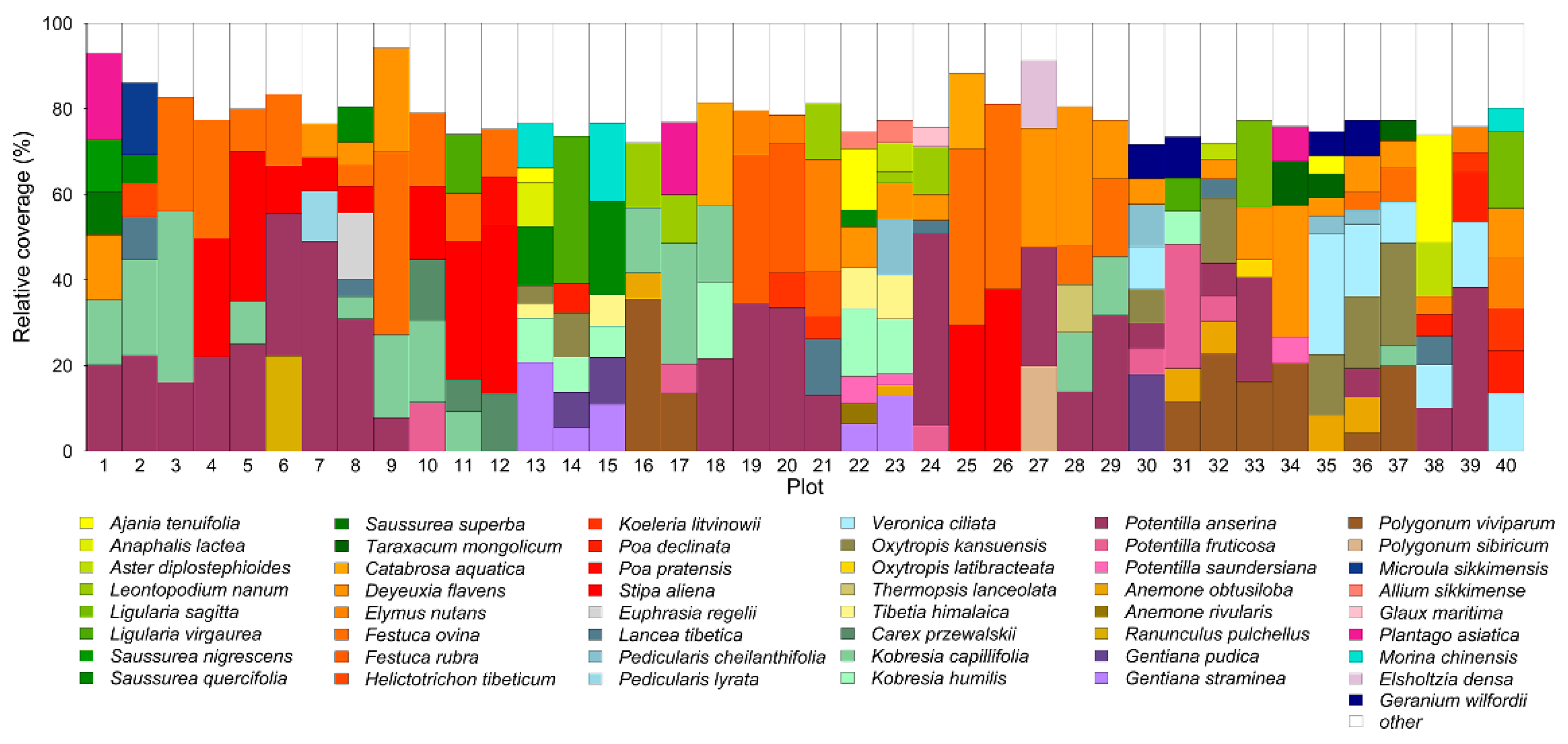
2.3. Field Data Collection

The field samples were collected on the same day as the UAV flight campaign, i.e., between 10 and 26 August 2021. At each survey site, we randomly set three 2 m × 2 m plots in a 100 m × 60 m range (Figure 1). The distance between any two plots was at least 15 m. We investigated the 1 m × 1 m area in the centre of each plot for species composition and species-wise coverage. To do so, we divided the 1 m2 quadrat into a grid of 100 squares each representing 1% cover and then estimate the percentage cover occupied by each species in the quadrat. We marked each plot in its centre for identification in images. In this research, we sampled species that accounted for the accumulative coverage of over 80% of the entire plot in each plot.
We collected 20 fully mature leaves of each sampled species at three vertical canopy positions along the plant stem: lower (n = 6), middle (n = 6) and upper (n = 8). We mixed the sampled leaves of each species and divided them into two equal subsamples. One subsample was quickly stored in liquid nitrogen for physiological trait measurement, and the other subsample was wrapped in wet tissue and stored in an icebox for structural trait measurement. For each sampled species, we randomly selected 5–10 mature and healthy individuals for the plant height measurement and calculated the average. In each plot, four 25 cm × 25 cm subplots at corners were clockwise numbered with the southern corner ranked 1 (Figure 1). Aboveground biomass in the subplots 1, 2 and 3; 2, 3 and 4; and 1, 3 and 4 of plots 1, 2 and 3, respectively, were harvested after the spectral measurements. In total, 40 out of 60 investigated plots were considered in this study (Figure 2). The relative coverage of each species in each plot was calculated based on these sampled species according to the following formula:
r c i = ( C i ) / j = 1 n C j
where rci represents the relative coverage of the ith species in a given plot, Ci is the coverage of the ith species, Cj is that of the jth species in the plot, and n is the total number of all species in the plot.

2.4. Foliar Trait Measurements and Plant Community Trait Calculation

In this study, we measured six biochemical traits including chlorophyll a content, chlorophyll b content, carotenoid content, nitrogen content, phosphorus content and starch content as well as four structural traits including plant height, leaf thickness, leaf dry matter content and specific leaf area (Table S1).
We measured chlorophyll a and b and carotenoid contents, as well as all structural traits, with the community weighted means approach. We determined chlorophyll a and b and carotenoid contents with a UV/VIS Spectrophotometer (UV-1800PC, Shanghai Mapada Instruments Co., Ltd., Shanghai, China). Except for the plant height, which was measured during the investigation, the other structural traits, such as leaf thickness, leaf dry matter content and specific leaf area, were measured on the same day of sampling. Leaf thickness was measured by a micrometre, and fresh weight was measured by an analytical balance. After leaf thickness measurement, we scanned leaves for the fresh leaf area with a flatbed scanner and then oven-dried those leaves at 65 °C for 72 h to a constant weight to determine the specific leaf area (fresh area/dried weight) and leaf dry matter content (dried weight/fresh weight).
We calculated the CWM values of chlorophyll a and b and carotenoid contents, plant height, leaf thickness, leaf dry matter content and specific leaf area according to the following formula:
t = ( i = 1 d t i × C i ) / i = 1 n C i
where t represents a community-level functional trait, ti denotes the functional trait of ith species, Ci is the coverage of ith species, d represents the total number of sampled species in a given plot and n is the total number of all species in a given plot.
In addition, we measured plant community nitrogen, phosphorus and starch contents using mixed samples. We shredded the harvested biomass, which was oven-dried at 65 °C for at least 72 h and homogenised it to mixed samples. The nitrogen content was analysed using an elemental analyser (Vario MACRO Cube, Frankfurt, Germany). The phosphorus content was measured by the molybdate–ascorbic acid method after H2SO4–H2O2 digestion [29]. Moreover, the starch content was measured by the anthrone colorimetric method using a UV/VIS Spectrophotometer (UV-1800PC, Shanghai Mapada Instruments Co., Ltd., Shanghai, China). Chlorophyll a, chlorophyll b and nitrogen contents were quantified in an area-based approach [30,31]. Area-based traits (mg/cm2) were calculated according to the following formula:
t r a i t a r e a = t r a i t m a s s / S L A

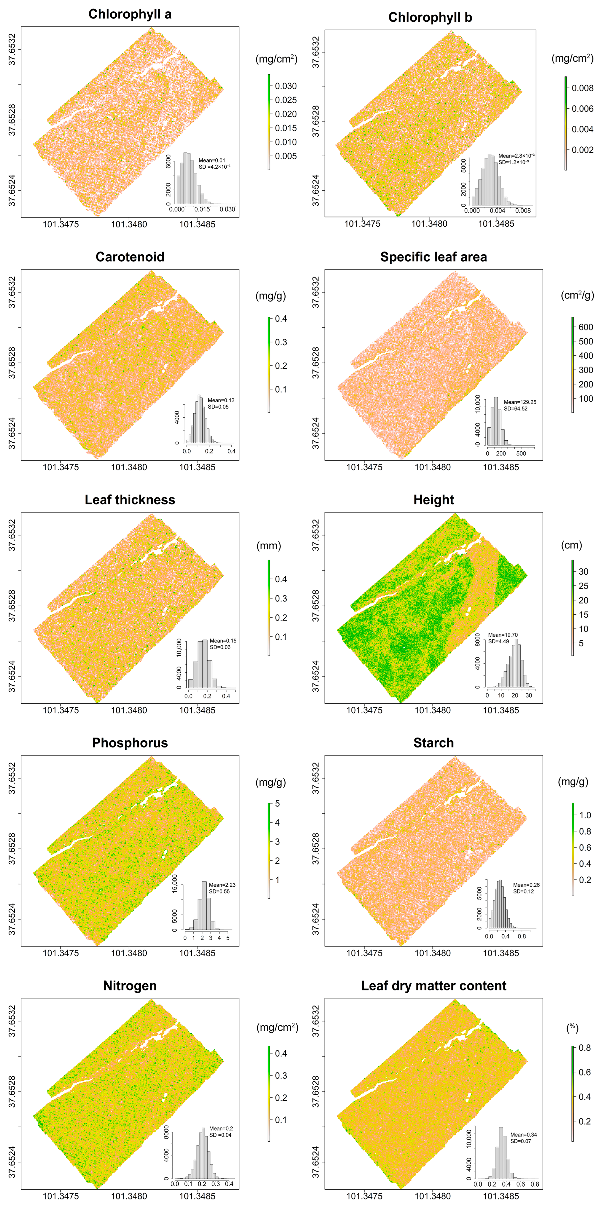
2.5. Mapping Plant Community Traits
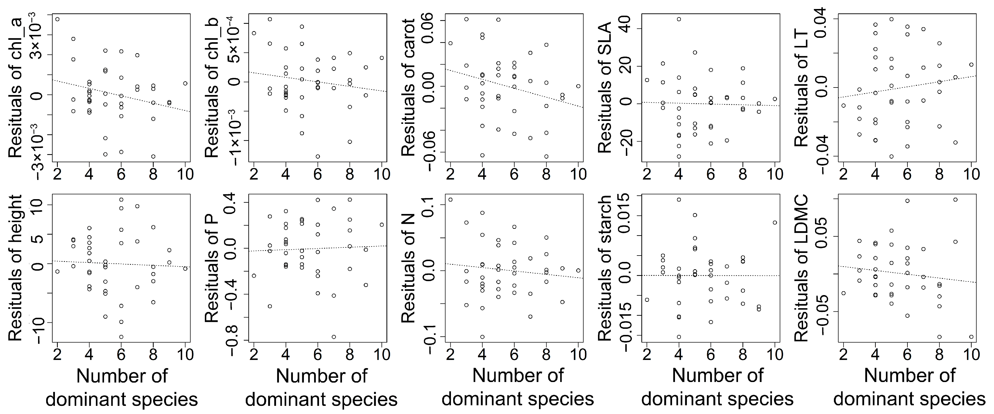
Here we tested four non-parametric models’ capability for the retrieval of various community-level traits (Figure 3). The two linear models are partial least square regression (PLSR) and the generic algorithm integrated with the PLSR (GA-PLSR). PLSR is a widely used algorithm in hyperspectral vegetation parameters retrieval [32,33]. As a model designed to incorporate multicollinearity problems, PLSR derives a smaller number of latent variables from the original data [34]. In this way, PLSR can eliminate the less informative variables but concentrate most explanatory variables on a few latent variables. However, the “large p-small n” problem (a large number of variables but a few samples) can still spoil the PLSR result [35]. In this condition, a variable selection pre-processing is known to improve PLSR performance [36]. Here, we adopted GA-PLSR which allows a band selection procedure in PLSR [37]. There are numerous studies showing GA-PLSR to be useful in promoting PLSR model performance [38,39]. It obeys the rule of biological evolution and natural selection to select informative features. Important features are able to survive after multiple iterations of model fitting and feature selection procedures. We selected random forest (RF) and extreme gradient boost (XGBoost) to evaluate nonlinear model performance in traits estimation. The RF model is one of the popular techniques of foliar trait prediction [40] and has been applied to map vegetation parameters at various scales [41,42]. XGBoost is an emerging machine learning algorithm showing satisfactory model performance in recent research [43].
In total, 40 plots were used as input for the four tested models. We used the leave-one-out-cross-validation (LOOCV) approach for model training and validation. Based on the pls package in R [44], we determined the number of latent factors used in PLSR for each community-level trait dataset by the predicted residual sum of squares (PRESS) statistic [45]. The feature selection of GA-PLSR was performed by the plsVarSel package in R [39]. After that, the standard PLSR routine was performed to determine the latent factors. As for the nonlinear models, we conducted a hyper-parameter optimisation process for each trait dataset (Table S2). RF models were performed with a randomforest package in R [46]. The number of trees (ntree, 100–1000 with the interval of 100) and the number of variables randomly sampled as candidates at each split (mtry, 1–125) were tuned, and each combination was replicated for 10 times to obtain the optimal parameters with the highest correlation coefficient. The XGBoost models were performed with the xgboost package in R [47], and the learning rate (eta, 0.1–1), maximum depth of a tree (max_depth, 0.1–1) and iteration rounds (nrounds, 1–100) were tuned to search for the best parameter in combination with the highest correlation coefficient.
We selected the model with the best performance for plant community trait mapping to visually represent plant community traits in space. Here we assessed the best model as a model with the highest R2 among all tested traits. To test whether the selected model could be adequately applied in a species-rich meadow, we further analysed the relationship between the predicted residuals of all plant community traits and the number of dominant species in each plot. To display spatial patterns of traits, we chose one image covering an area composed of a fenced meadow and a highly disturbed meadow. The location of this image was indicated in Figure 1. Thanks to the precise spatial resolution, we excluded non-vegetation pixels by supervised classification. The image was resampled into 50-cm spatial resolution by the nearest-neighbour algorithm (Figure S2). The relative uncertainty (standard deviation/mean) was calculated based on the 40 models generated from LOOCV. Data analysis was performed with R 4.1.0 [48].

3. Results

Among the biochemical traits, chlorophyll a and b, carotenoid and starch contents, showed good predictive accuracy, with the highest R2 value of four models ranging from 0.64~0.83. Phosphorus and nitrogen showed R2 values lower than 0.60 (Figure 4). As for the structural traits, specific leaf area (highest R2 = 0.70) and leaf thickness (highest R2 = 0.68) were both estimated well (Figure 4), while the estimates of plant height (R2 = 0.44) and leaf dry matter content (R2 = 0.30) were relatively poor.
Among four estimation models, GA-PLSR proved more accurate, as it produced the highest R2 value and the lowest nRMSE in most of the 10 plant community traits (Table 1). However, the other models displayed various performances in different traits. PLSR showed good performance in most traits, such as the biochemical traits related to photosynthesis (chlorophyll a and b and carotenoid contents) and specific leaf area. XGBoost owned model performance comparable with GA-PLSR for carotenoid content and plant height. However, it showed relatively low R2 values for nitrogen and starch contents. RF presented the worst predictive accuracy in most traits. Moreover, GA-PLSR had nRMSE values all below 0.4, while the other three models produced higher nRMSE values for most structural traits. Among the 10 traits, the model performance for leaf thickness, nitrogen content and starch content illustrated significant differences. The R2 values of different models varied from 0.68 to 0.04.
As for linear models, the model performance of PLSR increased significantly with band selection (GA-PLSR). In addition, GA-PLSR conquered the weakness of PLSR in some traits’ retrieval, such as nitrogen content, and yielded more satisfactory results than the two nonlinear models. For the two nonlinear models, XGBoost showed an obvious advantage over RF in all traits. However, the four tested models’ prediction of leaf dry matter content all below 0.4 made it the worst prediction among all 10 traits.
In addition, we analyzed the relationships between the predicted residuals of plant community traits and the number of dominant species in each plot. It showed that there was no statistically significant relationship (p > 0.05) between the predicted residuals of traits and the number of species (Figure 5).
Based on these results, we mapped spatial patterns of all tested traits, applying the GA-PLSR, as it exhibited stability and outperformed all models, to map traits (Figure 6). Our results showed that biochemical traits displayed more homogeneous distributions while structural traits, especially for plant height, had obvious spatial patterns. We calculated uncertainties from the predicted maps (Figure S3). For all traits, most uncertainty values were near zero.

4. Discussion

In this study, we predicted 10 significant plant community traits from the near-ground UAV-based hyperspectral image in a highly heterogeneous grassland with high species richness, with 9 traits producing moderate to good accuracies. Among all tested traits, chlorophyll a and b contents, carotenoid content, specific leaf area, leaf thickness and starch content could generate a predictive accuracy comparable to that of previous studies with R2 values greater than 0.60 [19].
The retrieval of plant height, phosphorus content and nitrogen content produced moderate predictive accuracy with R2 values varying from 0.44 to 0.54. This may be because the nonpigmented compounds of foliage and structure correlation intervals were mostly at longer wavelengths, while the detectable weak correlation could even be influenced by strong absorption of water content in fresh leaves [49,50]. Nevertheless, the R2 values of nitrogen and phosphorus content are comparable to other research in grasslands [18,19,51]. Similarly, all our tested models of leaf dry matter content produced poor predictive accuracies in this study, probably because leaf dry matter content reflected leaf water content. The distinct effect of foliar liquid water was at 1450 and 1950 nm, which was out of the available spectra range in this study [50]. This result suggested the relatively limited capacity of visible and near-infrared spectra in the retrieval of certain traits, which should be considered in future studies.
In this study, we tested four non-parametric models, including two linear models and two nonlinear models, in the direct retrieval of multiple traits. The results suggested that the predictive accuracy of some traits might be influenced to some extent by the choice of models. For example, an obvious increase of R2 was observed in starch content and leaf thickness when the linear model was applied. In contrast, a few traits yielded relatively consistent predictive accuracies across four models, such as plant height and carotenoid content.
As to the linear models, PLSR produced comparative average performance among all models but failed in some traits, such as nitrogen and leaf dry matter content. The better performance of GA-PLSR was consistent with some previous studies which confirmed the effects of feature selection in PLSR [52]. On the one hand, these significant improvements in model performance may because of the “large p–small n” problem. Since PLSR will make better use of all given features than nonlinear models, redundant variables may obscure truly usable bands [39]. As a result, PLSR with relatively limited training samples cannot handle hundreds of correlated bands well [53]. On the other hand, environmental and instrumental noise was inevitably mixed with spectral data, which may weaken the predictive accuracy.
We found that the performance of GA-PLSR was not sensitive to species richness, indicating its robustness in extracting information of functional traits based on the UAV hyperspectral imaging in a fine resolution. Therefore, GA-PLSR model could adequately estimate various plant community traits in species-rich alpine meadows.
Between two nonlinear models, XGBoost reported considerable advantages in predictive accuracy over RF. This result was consistent with recently published studies [43,54]. As XGBoost is effective in high-dimension data analysis, it is becoming a reliable method in vegetation parameter modelling using UAV-based hyperspectral data [52]. This may also provide a new option when conducting similar research facing nonlinear model selection.
Overall, GA-PLSR, the PLSR model using the GA feature selection approach, outperformed the other candidates for all tested traits in this research. The trade-off between complexity reduction and information preservation is a great challenge in hyperspectral data analysis. GA-PLSR can deal with estimations of various traits from canopy spectra with relatively satisfactory predictive accuracies. Maps generated from GA-PLSR depicted various patterns at the local level that could not be achieved only by site investigation. Meanwhile, the PLSR model combined with feature selection could serve as an option for researchers facing the “large p–small n” problem.

5. Conclusions

In this study, we investigated whether UAV-based hyperspectral imaging could be used to estimate 10 different plant functional traits at the community level in a species-rich alpine meadow ecosystem on the Qinghai–Tibet Plateau. In addition, we compared the performance of four non-parametric regression models, i.e., PLSR, GA-PLSR, RF and XGBoost. Based on the result, we conclude that the UAV-based hyperspectral image can be used to adequately estimate plant community traits in a species-rich alpine meadow with moderate to high accuracy. Specifically, we show that chlorophyll a, chlorophyll b, carotenoid content, starch content, specific leaf area and leaf thickness were estimated with good accuracies, with the highest R2 values between 0.64 (nRMSE = 0.16) and 0.83 (nRMSE = 0.11). While the estimation accuracies for nitrogen content, phosphorus content, plant height and leaf dry matter content were relatively low, with the highest R2 varying from 0.3 (nRMSE = 0.24) to 0.54 (nRMSE = 0.20). Among the four tested algorithms, the GA-PLSR produced the highest accuracy, followed by PLSR and XGBoost, and RF showed the poorest performance. Our study demonstrates the potential of UAV-based visible and near-infrared hyperspectral imagery to directly estimate various plant community traits in a natural grassland ecosystem at a fine scale.

Supplementary Materials

The following supporting information can be downloaded at: https://www.mdpi.com/article/10.3390/rs14143399/s1, Figure S1: Examples of corrected spectra of alpine meadow from five different flight sites. Figure S2: The UAV hyperspectral image used for mapping plant community traits. The upper one is the raw image and the lower one is the corrected image shown in true colour composites. This image covers plot 32, plot 33 and plot 34 in Figure 2. The white arrows indicate the location of the three reference panels. Figure S3: Frequency distribution of relative uncertainty of the 10 plant community trait maps produced by the GA_PLSR model. Table S1: Summary statistics of the 10 plant functional traits for sampled plots (n = 40). Table S2: An overview of optimal hyper-parameters of two machine learning models for 10 plant community traits.

Author Contributions

Conceptualization, Z.T.; methodology, Y.-W.Z., T.W. and Z.T.; formal analysis, Y.-W.Z. and Y.G.; investigation, Y.-W.Z., Z.Z., R.T. and S.S.; writing—original draft preparation, Y.-W.Z., T.W. and Y.G.; writing—review and editing, T.W., A.S. and Z.T.; supervision, T.W., A.S. and Z.T. All authors have read and agreed to the published version of the manuscript.

Funding

The study was funded by the Strategic Priority Research Programme of the Chinese Academy of Sciences (grant no. XDA26010102), the National Key Research and Development Program of China (grant no. 2019YFA0606602) and the National Natural Science Foundation of China (grant no. 32025025 & 31988102) to Z.T. The work of the first author (Y.-W.Z.) was carried out at the University of Twente while she was visiting the Netherlands as a joint doctoral student, funded by the China Scholarship Council (grant no. 202106010134). The work of the fourth author (A.S.) is partially supported by the Horizon 2020 research and innovation programme—European Commission ’BIOSPACE Monitoring Biodiversity from Space’ project (grant agreement ID 834709, H2020-EU.1.1).

Data Availability Statement

Not applicable.

Acknowledgments

We thank Yun-Hao Bai, Hong-Tu Zhang and Yiwei Lin for their valuable assistance during fieldwork.

Conflicts of Interest

The authors declare no conflict of interest.

References

  1. Violle, C.; Navas, M.-L.; Vile, D.; Kazakou, E.; Fortunel, C.; Hummel, I.; Garnier, E. Let the Concept of Trait Be Functional! Oikos 2007, 116, 882–892. [Google Scholar] [CrossRef]
  2. Laughlin, D.C.; Messier, J. Fitness of Multidimensional Phenotypes in Dynamic Adaptive Landscapes. Trends Ecol. Evol. 2015, 30, 487–496. [Google Scholar] [CrossRef] [PubMed]
  3. Wright, I.J.; Reich, P.B.; Westoby, M.; Ackerly, D.D.; Baruch, Z.; Bongers, F.; Cavender-Bares, J.; Chapin, T.; Cornelissen, J.H.C.; Diemer, M.; et al. The Worldwide Leaf Economics Spectrum. Nature 2004, 428, 821–827. [Google Scholar] [CrossRef] [PubMed]
  4. Díaz, S.; Lavorel, S.; de Bello, F.; Quétier, F.; Grigulis, K.; Robson, T.M. Incorporating Plant Functional Diversity Effects in Ecosystem Service Assessments. Proc. Natl. Acad. Sci. USA 2007, 104, 20684–20689. [Google Scholar] [CrossRef] [PubMed] [Green Version]
  5. Bruelheide, H.; Dengler, J.; Purschke, O.; Lenoir, J.; Jiménez-Alfaro, B.; Hennekens, S.M.; Botta-Dukát, Z.; Chytrý, M.; Field, R.; Jansen, F.; et al. Global Trait–Environment Relationships of Plant Communities. Nat. Ecol. Evol. 2018, 2, 1906–1917. [Google Scholar] [CrossRef]
  6. Gillison, A.N. Plant Functional Types and Traits at the Community, Ecosystem and World Level. In Vegetation Ecology; van der Maarel, E., Franklin, J., Eds.; John Wiley & Sons, Ltd.: Oxford, UK, 2013; pp. 347–386. ISBN 978-1-118-45259-2. [Google Scholar]
  7. Muscarella, R.; Uriarte, M. Do Community-Weighted Mean Functional Traits Reflect Optimal Strategies? Proc. R. Soc. B Biol. Sci. 2016, 283, 20152434. [Google Scholar] [CrossRef]
  8. Bjorkman, A.D.; Myers-Smith, I.H.; Elmendorf, S.C.; Normand, S.; Rüger, N.; Beck, P.S.A.; Blach-Overgaard, A.; Blok, D.; Cornelissen, J.H.C.; Forbes, B.C.; et al. Plant Functional Trait Change across a Warming Tundra Biome. Nature 2018, 562, 57–62. [Google Scholar] [CrossRef]
  9. Tang, Z.; Xu, W.; Zhou, G.; Bai, Y.; Li, J.; Tang, X.; Chen, D.; Liu, Q.; Ma, W.; Xiong, G.; et al. Patterns of Plant Carbon, Nitrogen, and Phosphorus Concentration in Relation to Productivity in China’s Terrestrial Ecosystems. Proc. Natl. Acad. Sci. USA 2018, 115, 4033–4038. [Google Scholar] [CrossRef] [Green Version]
  10. Ackerly, D.D.; Cornwell, W.K. A Trait-Based Approach to Community Assembly: Partitioning of Species Trait Values into within- and among-Community Components. Ecol. Lett. 2007, 10, 135–145. [Google Scholar] [CrossRef]
  11. Khalil, M.I.; Gibson, D.J.; Baer, S.G. Functional Response of Subordinate Species to Intraspecific Trait Variability within Dominant Species. J. Ecol. 2019, 107, 2040–2053. [Google Scholar] [CrossRef]
  12. Thenkabail, P.S.; Lyon, J.G.; Huete, A. (Eds.) Fundamentals, Sensor Systems, Spectral Libraries, and Data Mining for Vegetation: Hyperspectral Remote Sensing of Vegetation, 2nd ed.; CRC Press: Boca Raton, FL, USA, 2018; ISBN 978-1-315-16415-1. [Google Scholar]
  13. Pettorelli, N.; Wegmann, M.; Skidmore, A.; Mücher, S.; Dawson, T.P.; Fernandez, M.; Lucas, R.; Schaepman, M.E.; Wang, T.; O’Connor, B.; et al. Framing the Concept of Satellite Remote Sensing Essential Biodiversity Variables: Challenges and Future Directions. Remote Sens. Ecol. Conserv. 2016, 2, 122–131. [Google Scholar] [CrossRef]
  14. Homolová, L.; Malenovský, Z.; Clevers, J.G.P.W.; García-Santos, G.; Schaepman, M.E. Review of Optical-Based Remote Sensing for Plant Trait Mapping. Ecol. Complex. 2013, 15, 1–16. [Google Scholar] [CrossRef] [Green Version]
  15. Singh, A.; Serbin, S.P.; McNeil, B.E.; Kingdon, C.C.; Townsend, P.A. Imaging Spectroscopy Algorithms for Mapping Canopy Foliar Chemical and Morphological Traits and Their Uncertainties. Ecol. Appl. 2015, 25, 2180–2197. [Google Scholar] [CrossRef] [PubMed] [Green Version]
  16. Wang, R.; Gamon, J.A.; Emmerton, C.A.; Li, H.; Nestola, E.; Pastorello, G.Z.; Menzer, O. Integrated Analysis of Productivity and Biodiversity in a Southern Alberta Prairie. Remote Sens. 2016, 8, 214. [Google Scholar] [CrossRef] [Green Version]
  17. Asner, G.P.; Martin, R.E.; Anderson, C.B.; Knapp, D.E. Quantifying Forest Canopy Traits: Imaging Spectroscopy versus Field Survey. Remote Sens. Environ. 2015, 158, 15–27. [Google Scholar] [CrossRef]
  18. Zhao, Y.; Sun, Y.; Lu, X.; Zhao, X.; Yang, L.; Sun, Z.; Bai, Y. Hyperspectral Retrieval of Leaf Physiological Traits and Their Links to Ecosystem Productivity in Grassland Monocultures. Ecol. Indic. 2021, 122, 107267. [Google Scholar] [CrossRef]
  19. Wang, Z.; Townsend, P.A.; Schweiger, A.K.; Couture, J.J.; Singh, A.; Hobbie, S.E.; Cavender-Bares, J. Mapping Foliar Functional Traits and Their Uncertainties across Three Years in a Grassland Experiment. Remote Sens. Environ. 2019, 221, 405–416. [Google Scholar] [CrossRef]
  20. Li, C.; Wulf, H.; Schmid, B.; He, J.-S.; Schaepman, M.E. Estimating Plant Traits of Alpine Grasslands on the Qinghai-Tibetan Plateau Using Remote Sensing. IEEE J. Sel. Top. Appl. Earth Obs. Remote Sens. 2018, 11, 2263–2275. [Google Scholar] [CrossRef]
  21. Pajares, G. Overview and Current Status of Remote Sensing Applications Based on Unmanned Aerial Vehicles (UAVs). Photogramm. Eng. Remote Sens. 2015, 81, 281–330. [Google Scholar] [CrossRef] [Green Version]
  22. Rossi, C.; Kneubuehler, M.; Schuetz, M.; Schaepman, M.; Haller, R.; Risch, A. Spatial Resolution, Spectral Metrics and Biomass Are Key Aspects in Estimating Plant Species Richness from Spectral Diversity in Species-Rich Grasslands. Remote Sens. Ecol. Conserv. 2021, 8, 297–314. [Google Scholar] [CrossRef]
  23. de Castro, A.I.; Shi, Y.; Maja, J.M.; Peña, J.M. UAVs for Vegetation Monitoring: Overview and Recent Scientific Contributions. Remote Sens. 2021, 13, 2139. [Google Scholar] [CrossRef]
  24. Aasen, H.; Honkavaara, E.; Lucieer, A.; Zarco-Tejada, P.J. Quantitative Remote Sensing at Ultra-High Resolution with UAV Spectroscopy: A Review of Sensor Technology, Measurement Procedures, and Data Correction Workflows. Remote Sens. 2018, 10, 1091. [Google Scholar] [CrossRef] [Green Version]
  25. Jetz, W.; Cavender-Bares, J.; Pavlick, R.; Schimel, D.; Davis, F.W.; Asner, G.P.; Guralnick, R.; Kattge, J.; Latimer, A.M.; Moorcroft, P.; et al. Monitoring Plant Functional Diversity from Space. Nat. Plants 2016, 2, 16024. [Google Scholar] [CrossRef] [Green Version]
  26. Zhang, C.; Willis, C.G.; Klein, J.A.; Ma, Z.; Li, J.; Zhou, H.; Zhao, X. Recovery of Plant Species Diversity during Long-Term Experimental Warming of a Species-Rich Alpine Meadow Community on the Qinghai-Tibet Plateau. Biol. Conserv. 2017, 213, 218–224. [Google Scholar] [CrossRef]
  27. Hadley, B.C.; Garcia-Quijano, M.; Jensen, J.R.; Tullis, J.A. Empirical versus Model-based Atmospheric Correction of Digital Airborne Imaging Spectrometer Hyperspectral Data. Geocarto Int. 2005, 20, 21–28. [Google Scholar] [CrossRef]
  28. Arroyo-Mora, J.P.; Kalacska, M.; Løke, T.; Schläpfer, D.; Coops, N.C.; Lucanus, O.; Leblanc, G. Assessing the Impact of Illumination on UAV Pushbroom Hyperspectral Imagery Collected under Various Cloud Cover Conditions. Remote Sens. Environ. 2021, 258, 112396. [Google Scholar] [CrossRef]
  29. Jones, J.B., Jr. Laboratory Guide for Conducting Soil Tests and Plant Analysis; CRC press: New York, NY, USA, 2001; ISBN 1-4200-2529-5. [Google Scholar]
  30. Roelofsen, H.D.; Van Bodegom, P.M.; Kooistra, L.; Witte, J.-P.M. Trait Estimation in Herbaceous Plant Assemblages from in Situ Canopy Spectra. Remote Sens. 2013, 5, 6323–6345. [Google Scholar] [CrossRef]
  31. Wang, Z.; Skidmore, A.K.; Darvishzadeh, R.; Heiden, U.; Heurich, M.; Wang, T. Leaf Nitrogen Content Indirectly Estimated by Leaf Traits Derived From the PROSPECT Model. IEEE J. Sel. Top. Appl. Earth Obs. Remote Sens. 2015, 8, 3172–3182. [Google Scholar] [CrossRef]
  32. Schweiger, A.K.; Cavender-Bares, J.; Townsend, P.A.; Hobbie, S.E.; Madritch, M.D.; Wang, R.; Tilman, D.; Gamon, J.A. Plant Spectral Diversity Integrates Functional and Phylogenetic Components of Biodiversity and Predicts Ecosystem Function. Nat. Ecol. Evol. 2018, 2, 976–982. [Google Scholar] [CrossRef]
  33. Durán, S.M.; Martin, R.E.; Díaz, S.; Maitner, B.S.; Malhi, Y.; Salinas, N.; Shenkin, A.; Silman, M.R.; Wieczynski, D.J.; Asner, G.P.; et al. Informing Trait-Based Ecology by Assessing Remotely Sensed Functional Diversity across a Broad Tropical Temperature Gradient. Sci. Adv. 2019, 5, eaaw8114. [Google Scholar] [CrossRef] [Green Version]
  34. Rosipal, R.; Krämer, N. Overview and Recent Advances in Partial Least Squares. In Subspace, Latent Structure and Feature Selection; Saunders, C., Grobelnik, M., Gunn, S., Shawe-Taylor, J., Eds.; Lecture Notes in Computer Science; Springer: Berlin, Heidelberg, Germany, 2006; Volume 3940, pp. 34–51. ISBN 978-3-540-34137-6. [Google Scholar]
  35. Mehmood, T.; Liland, K.H.; Snipen, L.; Sæbø, S. A Review of Variable Selection Methods in Partial Least Squares Regression. Chemom. Intell. Lab. Syst. 2012, 118, 62–69. [Google Scholar] [CrossRef]
  36. Dormann, C.F.; Elith, J.; Bacher, S.; Buchmann, C.; Carl, G.; Carré, G.; Marquéz, J.R.G.; Gruber, B.; Lafourcade, B.; Leitão, P.J.; et al. Collinearity: A Review of Methods to Deal with It and a Simulation Study Evaluating Their Performance. Ecography 2013, 36, 27–46. [Google Scholar] [CrossRef]
  37. Hasegawa, K.; Miyashita, Y.; Funatsu, K. GA Strategy for Variable Selection in QSAR Studies: GA-Based PLS Analysis of Calcium Channel Antagonists. J. Chem. Inf. Comput. Sci. 1997, 37, 306–310. [Google Scholar] [CrossRef]
  38. Santos-Rufo, A.; Mesas-Carrascosa, F.-J.; García-Ferrer, A.; Meroño-Larriva, J.E. Wavelength Selection Method Based on Partial Least Square from Hyperspectral Unmanned Aerial Vehicle Orthomosaic of Irrigated Olive Orchards. Remote Sens. 2020, 12, 3426. [Google Scholar] [CrossRef]
  39. Mehmood, T.; Sæbø, S.; Liland, K.H. Comparison of Variable Selection Methods in Partial Least Squares Regression. J. Chemom. 2020, 34, e3226. [Google Scholar] [CrossRef] [Green Version]
  40. Moreno-Martínez, Á.; Camps-Valls, G.; Kattge, J.; Robinson, N.; Reichstein, M.; van Bodegom, P.; Kramer, K.; Cornelissen, J.H.C.; Reich, P.; Bahn, M.; et al. A Methodology to Derive Global Maps of Leaf Traits Using Remote Sensing and Climate Data. Remote Sens. Environ. 2018, 218, 69–88. [Google Scholar] [CrossRef] [Green Version]
  41. Loozen, Y.; Rebel, K.T.; de Jong, S.M.; Lu, M.; Ollinger, S.V.; Wassen, M.J.; Karssenberg, D. Mapping Canopy Nitrogen in European Forests Using Remote Sensing and Environmental Variables with the Random Forests Method. Remote Sens. Environ. 2020, 247, 111933. [Google Scholar] [CrossRef]
  42. Chemura, A.; Mutanga, O.; Odindi, J.; Kutywayo, D. Mapping Spatial Variability of Foliar Nitrogen in Coffee (Coffea arabica L.) Plantations with Multispectral Sentinel-2 MSI Data. ISPRS J. Photogramm. Remote Sens. 2018, 138, 1–11. [Google Scholar] [CrossRef]
  43. Yang, X.; Yang, R.; Ye, Y.; Yuan, Z.; Wang, D.; Hua, K. Winter Wheat SPAD Estimation from UAV Hyperspectral Data Using Cluster-Regression Methods. Int. J. Appl. Earth Obs. Geoinf. 2021, 105, 102618. [Google Scholar] [CrossRef]
  44. Mevik, B.-H.; Wehrens, R. The Pls Package: Principal Component and Partial Least Squares Regression in R. J. Stat. Softw. 2007, 18, 1–23. [Google Scholar] [CrossRef] [Green Version]
  45. Chen, S.; Hong, X.; Harris, C.J.; Sharkey, P.M. Sparse Modeling Using Orthogonal Forward Regression with PRESS Statistic and Regularization. IEEE Trans. Syst. Man Cybern. Part B 2004, 34, 898–911. [Google Scholar] [CrossRef] [PubMed]
  46. Breiman, L. Random Forests. Mach. Learn. 2001, 45, 5–32. [Google Scholar] [CrossRef] [Green Version]
  47. Chen, T.; He, T.; Benesty, M.; Khotilovich, V.; Tang, Y.; Cho, H.; Chen, K.; Mitchell, R.; Cano, I.; Zhou, T.; et al. xgboost: Extreme Gradient Boosting; R Package Version 1.6.0.1; 2022; Available online: https://CRAN.R-project.org/package=xgboost (accessed on 24 May 2022).
  48. R Core Team. R: A Language and Environment for Statistical Computing; R Core Team: Vienna, Austria, 2019. [Google Scholar]
  49. Ferwerda, J.G.; Skidmore, A.K.; Mutanga, O. Nitrogen Detection with Hyperspectral Normalized Ratio Indices across Multiple Plant Species. Int. J. Remote Sens. 2005, 26, 4083–4095. [Google Scholar] [CrossRef]
  50. Ollinger, S.V. Sources of Variability in Canopy Reflectance and the Convergent Properties of Plants. New Phytol. 2011, 189, 375–394. [Google Scholar] [CrossRef] [PubMed]
  51. Ramoelo, A.; Skidmore, A.K.; Cho, M.A.; Schlerf, M.; Mathieu, R.; Heitkönig, I.M.A. Regional Estimation of Savanna Grass Nitrogen Using the Red-Edge Band of the Spaceborne RapidEye Sensor. Int. J. Appl. Earth Obs. Geoinf. 2012, 19, 151–162. [Google Scholar] [CrossRef]
  52. Zhang, J.; Cheng, T.; Guo, W.; Xu, X.; Qiao, H.; Xie, Y.; Ma, X. Leaf Area Index Estimation Model for UAV Image Hyperspectral Data Based on Wavelength Variable Selection and Machine Learning Methods. Plant Methods 2021, 17, 49. [Google Scholar] [CrossRef]
  53. Rivera-Caicedo, J.P.; Verrelst, J.; Muñoz-Marí, J.; Camps-Valls, G.; Moreno, J. Hyperspectral Dimensionality Reduction for Biophysical Variable Statistical Retrieval. ISPRS J. Photogramm. Remote Sens. 2017, 132, 88–101. [Google Scholar] [CrossRef]
  54. Zhao, X.; Pan, X.; Ma, Y.; Yan, W. Research on Forage Hyperspectral Image Recognition Based on F-SVD and XGBoost. MATEC Web Conf. 2021, 336, 06027. [Google Scholar] [CrossRef]
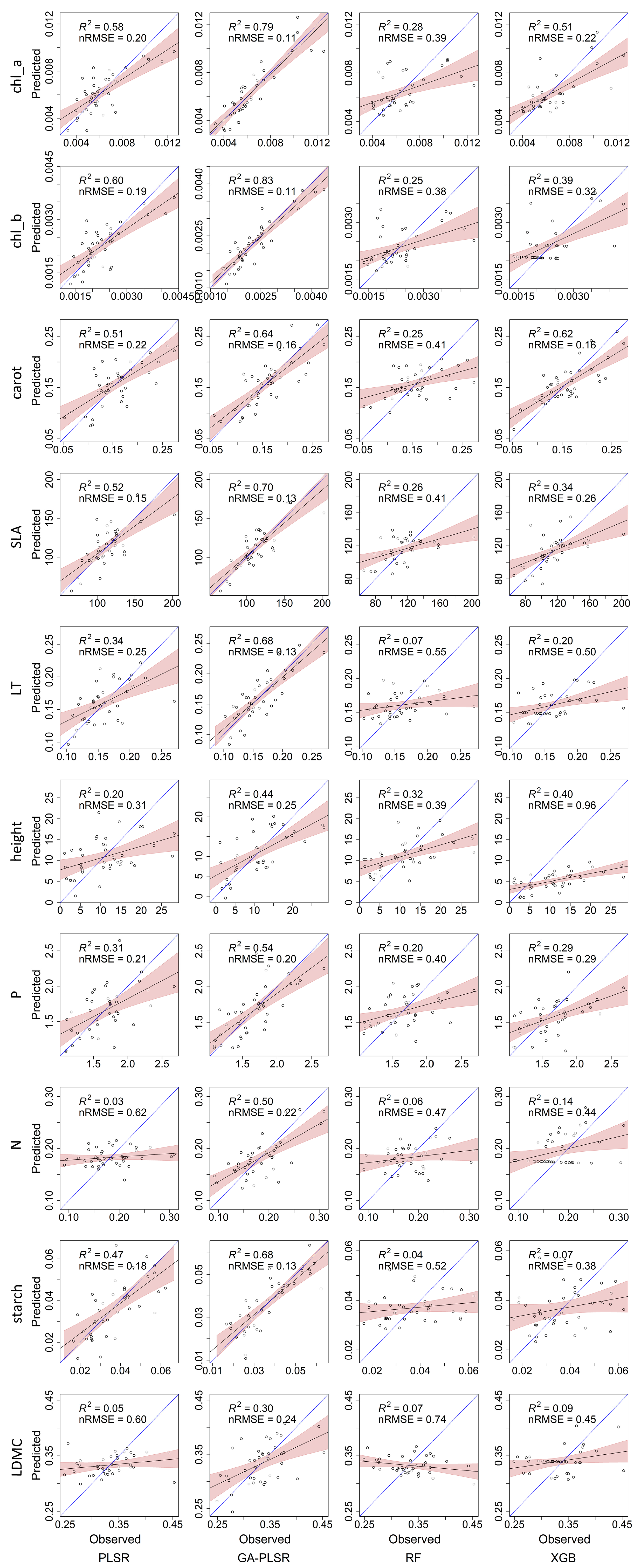
Figure 1. (A) Location of the study area on the Qinghai–Tibet Plateau; (B) photo of the study area; (C) study area with the location of used UAV flight sites; and (D) sampling design for each site in which the red boxes denote the three 2 m × 2 m sampling plots, and the green (25 cm × 25 cm), blue (50 cm × 50 cm) and purple (1 m × 1 m) boxes denote the quadrats for biomass harvesting, UAV spectra extraction and species survey, respectively, in each plot. Aboveground biomass in the subplots 1, 2 and 3; 2, 3 and 4; and 1, 3 and 4 for plots 1, 2 and 3, respectively, were harvested after the spectral measurements.
Remotesensing 14 03399 g001
Figure 2. The sampled species composition and relative coverage in the 1 m × 1 m area (corresponding to the purple boxes in Figure 1D) in each plot used in this study.
Remotesensing 14 03399 g002
Figure 3. Overview of the study workflow.
Remotesensing 14 03399 g003
Figure 4. Predicted versus observed chlorophyll a (chl_a), chlorophyll b (chl_b), carotenoid (carot), specific leaf area (SLA), leaf thickness (LT), plant height (height), phosphorus content (P), starch content (starch), leaf dry matter content (LDMC) and nitrogen content (N) from PLSR, GA-PLSR, RF and XGBoost; the blue line denotes the 1:1 line, and the red areas denote the 95% confidence interval.
Remotesensing 14 03399 g004
Figure 5. Relationships between the predicted residuals of plant community traits and the number of dominant species in each plot. Dotted lines denote non-significant relationships (p > 0.05): chl_a, chlorophyll a; chl_b, chlorophyll b; carot, carotenoid; SLA, specific leaf area; LT, leaf thickness; height, plant height; P, phosphorus content; N, nitrogen content; starch, starch content; LDMC, leaf dry matter content.
Remotesensing 14 03399 g005
Figure 6. Spatial patterns of plant community traits mapped using GA-PLSR and the frequency distribution of pixel values. The location of this image was indicated in Figure 1. This image covers plot 32, plot 33 and plot 34 in Figure 2.
Remotesensing 14 03399 g006
Table 1. Model evaluation and comparison of the coefficient of determination (R-squared) and normalised root mean-square error (nRMSE) on 10 plant community traits.
TraitPLSRGA-PLSRRFXGBoost
R2nRMSER2nRMSER2nRMSER2nRMSE
chlorophyll a0.5820.3%0.7910.7%0.2838.7%0.5122.0%
chlorophyll b0.6018.5%0.8310.7%0.2537.9%0.3932.0%
carotenoid0.5122.2%0.6416.0%0.2540.7%0.6215.8%
specific leaf area0.5215.1%0.7012.8%0.2641.3%0.3425.6%
leaf thickness0.3424.5%0.6813.5%0.0755.3%0.2050.0%
plant height0.2031.4%0.4425.3%0.3239.3%0.4095.7%
phosphorus content0.3120.7%0.5419.5%0.2040.3%0.2928.7%
nitrogen content0.0362.0%0.5022.3%0.0647.3%0.1444.1%
starch content0.4718.4%0.6813.5%0.0451.9%0.0737.6%
leaf dry matter content0.0559.8%0.3024.2%0.0774.4%0.0944.9%
Publisher’s Note: MDPI stays neutral with regard to jurisdictional claims in published maps and institutional affiliations.

