Article

Machine Learning in the Analysis of Multispectral Reads in Maize Canopies Responding to Increased Temperatures and Water Deficit

1
Faculty of Electrical Engineering, Computer Science and Information Technology, Josip Juraj Strossmayer University of Osijek, HR31000 Osijek, Croatia
2
Agricultural Institute Osijek, HR31000 Osijek, Croatia
*
Author to whom correspondence should be addressed.
Remote Sens. 2022, 14(11), 2596; https://doi.org/10.3390/rs14112596
Submission received: 29 April 2022 / Revised: 19 May 2022 / Accepted: 26 May 2022 / Published: 28 May 2022
(This article belongs to the Special Issue Remote Sensing of Vegetation Function and Traits)

Abstract

:
Real-time monitoring of crop responses to environmental deviations represents a new avenue for applications of remote and proximal sensing. Combining the high-throughput devices with novel machine learning (ML) approaches shows promise in the monitoring of agricultural production. The 3 × 2 multispectral arrays with responses at 610 and 680 nm (red), 730 and 760 nm (red-edge) and 810 and 860 nm (infrared) spectra were used to assess the occurrence of leaf rolling (LR) in 545 experimental maize plots measured four times for calibration dataset (n = 2180) and 145 plots measured once for external validation. Multispectral reads were used to calculate 15 simple normalized vegetation indices. Four ML algorithms were assessed: single and multilayer perceptron (SLP and MLP), convolutional neural network (CNN) and support vector machines (SVM) in three validation procedures, which were stratified cross-validation, random subset validation and validation with external dataset. Leaf rolling occurrence caused visible changes in spectral responses and calculated vegetation indexes. All algorithms showed good performance metrics in stratified cross-validation (accuracy >80%). SLP was the least efficient in predictions with external datasets, while MLP, CNN and SVM showed comparable performance. Combining ML with multispectral sensing shows promise in transition towards agriculture based on data-driven decisions especially considering the novel Internet of Things (IoT) avenues.

1. Introduction

Human population growth has led to increasing food requirements and resource depletion, intensifying the use of modern technologies in agriculture over the last few decades. Thus, major achievements in sensing technologies, wireless communication and artificial intelligence have been made by research efforts in agriculture globally [1,2]. In the context of climate change, real-time monitoring of drought is of primary interest which yielded a forked remote sensing approach, deploying satellite imagery to spot drought occurrence [3,4,5,6,7], or utilizing the recent developments in affordable sensor solutions, generating data in a more (unmanned aerial vehicles—UAV) or less (pole, machine or tower mounted) remote manner [8,9,10,11,12]. In conventional agricultural production, the only objective data collected on plant side (grain yield) are collected when the plant is already dead, so the real-time monitoring practices represent a paradigmatic shift for most farmers around the world.
Studies show that there is a growing occurrence of heatwave days accompanied by longer spans of drought [13]. These deleterious climate changes come with increased sensitivity of maize and soybean to heat and drought, despite ever strong breeding efforts for tolerance to abiotic stress [14]. In maize, there is a large number of morpho-physiological adjustments in response to drought stress [15,16,17]. However, many of these changes are irreversible, such as low fertilization rate, increased susceptibility to diseases or depleted stands [18], and once they are expressed, the economic losses are unavoidable. There are also some changes that are different among maize cultivars [19] and they are reversible in nature providing an excellent signal of the current plant water status.
One such trait is transverse rolling of leaf blades (Figure S1), usually caused by hydronastic changes. Many plant species use this mechanism as a drought avoidance strategy [20]. It represents a mechanism of adaptation in plants to control stress mostly by the means of auto-stress (cell-wall tension increase/decrease), reduction in the light interception and transpiration, thus preventing dehydration and overheating [21]. Not all genotypes express leaf rolling at the same conditions [22,23], nor the monotonic increase in leaf curvature shows the same maximum over different genotypes [24]. While in some genotypes it represents an avoidance strategy for stress conditions, in others it marks a tipping point for the physiological damage [25,26,27], thus implying the need to dynamically monitor for this trait in real time, for breeding and management purposes. So far, the use of different methods of leaf rolling quantification was reported in the literature, most of them grading responses in scales from 1 (no leaf rolling) to 5 (completely rolled leaves, dead or lax) [28,29,30], or 1 (no leaf rolling) to 9 (completely rolled leaf blades) [31]. All of the mentioned methods imply phenotyping at (i) drought stress treatment, or (ii) at the time of solar noon, when the strongest leaf rolling is expected to occur [24]. However, all of the conventional methods also imply a need for human screening limiting the ability to capture trait dynamics, accompanied with the increased error in rolling grading between scorers. In order to use phenotypic indicators, such as leaf rolling in some unfavorable conditions, in decision support systems, the possibility for their remote monitoring is of critical importance.
Leaf rolling causes several easily detectable changes in plant level. One such change is reduction in leaf area index (LAI), rendering the changes easily detectable by simple hemispherical photography [31]. However, there are also more subtle changes in spectral derivatives of leaf-rolled plants exposed to drought treatment, mostly caused by the accumulation/translocation of biochemicals and decrease in photosynthetic activity [32], allowing the drought detection using hyperspectral data along with several derived normalized vegetation indexes such as normalized difference vegetation index (NDVI) [33]. Normalized difference vegetation index and other normalized vegetation indices (VI) represent a useful and sensitive tool in vegetation monitoring converting the raw sensor reads to useful normalized and repeatable results [34,35]. Hyper/multispectral monitoring is already a proven method of vegetation monitoring [36,37] coming more and more to focus of researchers addressing high-throughput phenotyping and precision agriculture [38,39,40]. Moreover, different types of stress can be detected by combining ML with spectral monitoring [41,42,43]. There are many approaches for applied regression analysis of the remote sensing data being used [44,45]; however, such models are inefficient when accounting for nonlinearity of targets in multi-dimensional hyperplanes. On the other hand, these data properties are efficiently handled by modern machine learning (ML) algorithms, extracting numerical features from the data while retaining the information from the original dataset. Moreover, there is a growing body of evidence of the superiority in performance of ML algorithms in remote sensing data analysis for various agricultural applications such as vegetation classification [46], biomass and soil moisture analysis [47], crop stress phenotyping [38], precision farming [48,49] and many others [50]. Furthermore, these methods also have an ecological and humanitarian depth showing promise in helping to adhere to the Sustainable Development Goals [51] presented by the United Nations [52].
In this research, we attempted to use a low-cost sensor capturing spectral responses around several critical plant reflectance wavelengths and to apply machine learning to detect changes in plant morphology for the envisioned use in precision agriculture and plant breeding. Specifically, objectives were to determine the usefulness of a simple multispectral sensor to monitor leaf rolling in maize as a sign of stress, and to assess different machine learning models readily applied in the classification of labeled data.

2. Materials and Methods

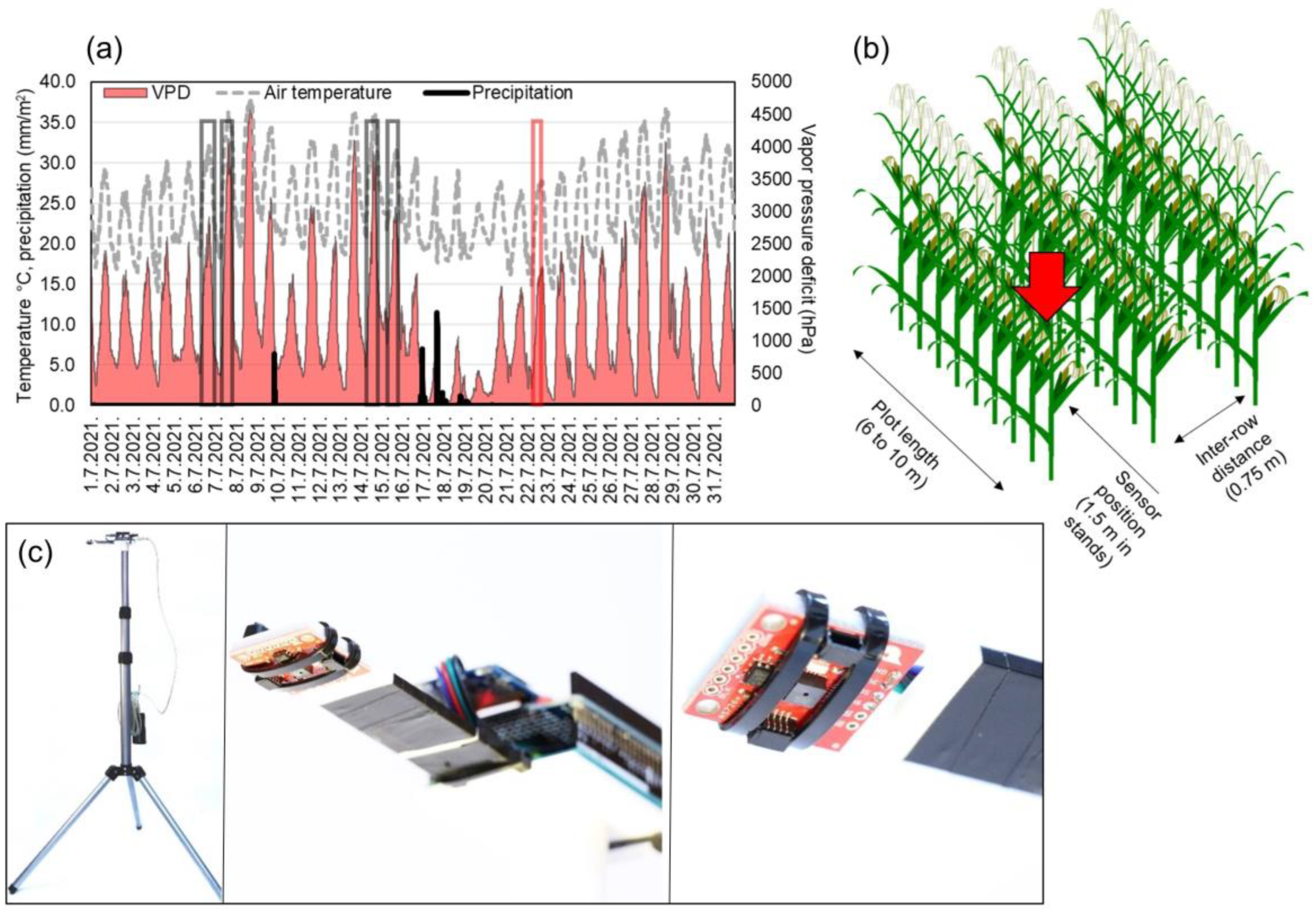
2.1. Field Experiments

The field experiments were carried out at the experimental station of the Agricultural Institute Osijek (AIO) in Osijek Croatia (45°32′N 18°44′E). Fields are subject to barley–soybean–maize rotation and are, following the soil analysis, fertilized and maintained with non-limiting amounts of fertilizers following respective local best practices and regulations. For the purpose of development of new cultivars AIO organizes several levels of field trials with multiple cultivars, separated between early, early to medium, medium to late and late maturity breeding programs. Maturity was categorized by FAO system [53] with reference genotypes used as checks to categorize hybrids to groups 1 (early) to 7 (late). Besides breeding programs, AIO organizes demonstrational trials with 3 to 75 hybrids representing the pallet of latest breeding efforts. AIO is a certified seed producer, marketing maize hybrids in Southeast and Central Europe and the Middle East. Thus, there is a considerable diversity of hybrids present at breeding trials of every maturity group, aiming at adaptation to different agro-ecological scenarios. For the purpose of this study, we chose seven trials with different numbers of hybrids from the mentioned maturity groups, namely, single irrigated demonstrational trial (DTir) and two rainfed demonstrational trials (DTrf and SDTrf). Soil type in DTrf and DTir was anthropogenized eutric cambisol, while at SDTrf, soil was sandy loam. In the gradient of trial qualities, SDTrf thus represented a low-water availability trial, while DTir was not water limited during the screening. The DTir trial was irrigated twice with 40 mm/m2 per irrigation, on 20th of June and 2nd of July. Irrigation was carried out by gear-driven full circle sprinklers. Trials of early (ET), early to medium (EMT), medium to late (MLT) and late maturity (LT) breeding programs were represented by randomized complete block trials with 25 hybrids in four replicates on anthropogenized eutric cambisol (ET, MLT and LT) and sandy loam (EMT). All trials were sown in a north–south orientation except SDTrf and EMT which were sown in an east–west orientation. Details on experimental design are shown in Table 1.

2.2. Measurements and Agroecological Conditions

Measurements were carried out with AMS (ams-OSRAM AG, Austria) AS7263 sensor unit with six spectral bands (3 × 2 photo diode array) responsive to wavelengths in red and near-infrared spectra (610, 680, 730, 760, 810 and 860 nm) with 20 nm full width at half maximum. Sensor consists of plastic housing, a lens and photodiode array with aperture of 0.75 mm and 20.5° viewing angle. The sensor was connected to Arduino Uno prototyping board and the data were logged based on a programmed button-interrupt to SD card. Each interrupt consisted of 10 consecutive measurements within 2000 ms and their average was logged with timestamp. The wiring was mounted to a 3D printer printed mount and set up on a 2.2 m telescopic tripod, and the 10 Ah power bank was used to power the device (Figure 1c). The sensor was set 2 m from ground at 90° to capture leaves in 0.6 m2 of theoretical field width (to ground). The 2 m height was chosen as only 16 out of 545 plots showed height lower than 2 m (shortest hybrid in SDTrf was 1.77 m), so the sensor captured the leaves intersecting the field of view. Measurements were carried out during the morning and around solar noon (Figure 1a), when the weakest and the strongest leaf rolling is expected to occur (Table 1) [31]. The tripod with mounted sensor wiring was carried between the plots and set 1.5 m within rows for measurement (Figure 1b). The exact data for plant height were collected for three experiments DTir, DTrf and SDTrf with 3 m long ruler, and no connection was observed between multispectral reads and plant height (correlations < 0.3). The mean height was 214.9 cm, with standard deviation of 6.05 cm.
All 545 plots (Table 1) were assessed for four times with a sensor and labeled by a maize breeder for leaf rolling, two times during the morning and two times in the solar noon (Figure 1a) on sunny days, yielding 2180 labeled measurements and means of sensor reads. Additionally, DTir, DTrf and SDRtf were assessed on 22nd of July, to obtain an external validation set for testing the robustness of the modelling approach.
Timing of measurements (Figure 1a) was chosen to capture the window of highest maize susceptibility to drought [54], heat [55] and the combination of these two stressors. This window covers growth stages from floral transition to early grain filling. During the experiments, different hybrids transitioned between developmental stages; however, the aim of this study was not to analyze genotypic responses but rather the ability of a simple multispectral sensor to capture leaf rolling occurrence. Initial grades of leaf rolling (samples available as Supplementary Figure S1) were taken following methodology described in Bolaños and Edmeades [30] on scale 1 (green erect leaf blades) to 5 (rolled, lax or dead). However, the experimental design limited appropriate account for all factors affecting the rolling occurrence. Furthermore, as the leaf morphology affects the rolling maximum [24], the lower grades (higher than 1) also indicate leaf rolling, whose occurrence was of primary interest of this study. Reads were thus binary labeled with 0 for no leaf rolling (below 15% of the plants within the plot showing leaf rolling) and 1 (more than 15% of the plants within the plot showing leaf rolling). The 15% threshold represents the tolerable amount of secondary plants that are usually more susceptible to leaf rolling. The images of leaf-rolled plants in the field are available as Figure S1.

2.3. Data Analysis and Model Assesment

Six raw sensor reads were used to calculate 15 unique, simple vegetation indexes (VI). The indexes were calculated as absolute values of the quotient between differences of the subtracted and added values of each two pairs of wavelengths ( w l a f ):
V I i = | w l b w l a w l a + w l b |
The raw sensor reads and VIs were scaled, centered and log-transformed and the principal component analysis (PCA) was carried out in R [56]. The raw sensor reads and the VI values (21 original features) were tested for differences between LR+ and LR− by the means of a Welch two-sample t-test. Prior to tests, the data were visually assessed for normality of distribution densities. The raw data and VIs were read into Python environment and four machine learning models were constructed. First model was the single layer perceptron (SLP) with single fully connected layer with 128 nodes with rectified linear unit (ReLu) activation function. The dense neural network layer was flattened and passed through softmax function to obtain predictions. For multilayer perceptron (MLP), another hidden layer was added with 32 fully connected nodes prior to flattening. Convolutional neural network (CNN) was setup with single 1D convolution layer of length 64, followed by two hidden fully connected layers with 48 and 24 nodes before flattening and passing to the softmax function (Figure 2). These three models were setup in TensorFlow library with training in 100 epochs with batch size of 16. Additionally, a support vector machine (SVM) model was built with scikit-learn module svm with linear kernel and penalty of the error term (C) set to 1. Three procedures of model validation were followed using calibration (n = 2180) and external (n = 145) labeled datasets:
  • Stratified 5-fold cross-validation with 85% (1853) of the 2180 records;
  • Validation based on a 15% random subset (327) of the 2180 records with random seed number 109;
  • Validation with an external validation set consisting of 145 separate records.
To ensure reproducibility of the results, the same subsets were used to validate each model.
The model performance was assessed by model accuracy and its standard deviation across folds in cross-validation, and by measuring accuracy, precision and recall in random-subset validation and validation with external dataset. The breeder’s classifications at solar noon (explained above) to LR− and LR+ were used as ground truth in model evaluation metrics. The performance indicators were calculated as:
A c c u r a c y = T N + T P n ,   P r e c i s i o n = T P T P + F P ,   R e c a l l = T P T P + F N  
where TN is number of true negatives, TP is number of true positives, FP is a number of false positives, FN is number of false negatives and n is a number of relevant samples. Furthermore, F1 score was calculated as
F 1 = 2 P r e c i s i o n R e c a l l P r e c i s i o n + R e c a l l
F1 score represents a harmonic mean between the ability of a model to classify true positives among all positively labeled examples (precision) and the fraction of examples classified as positives among all positive plots (recall).
The CPU time was assessed on an Intel® i7 9750H 6-core, 12-thread processor with 12 MB internal cache memory. Full notebook with Python code is available from the corresponding author upon request.

3. Results

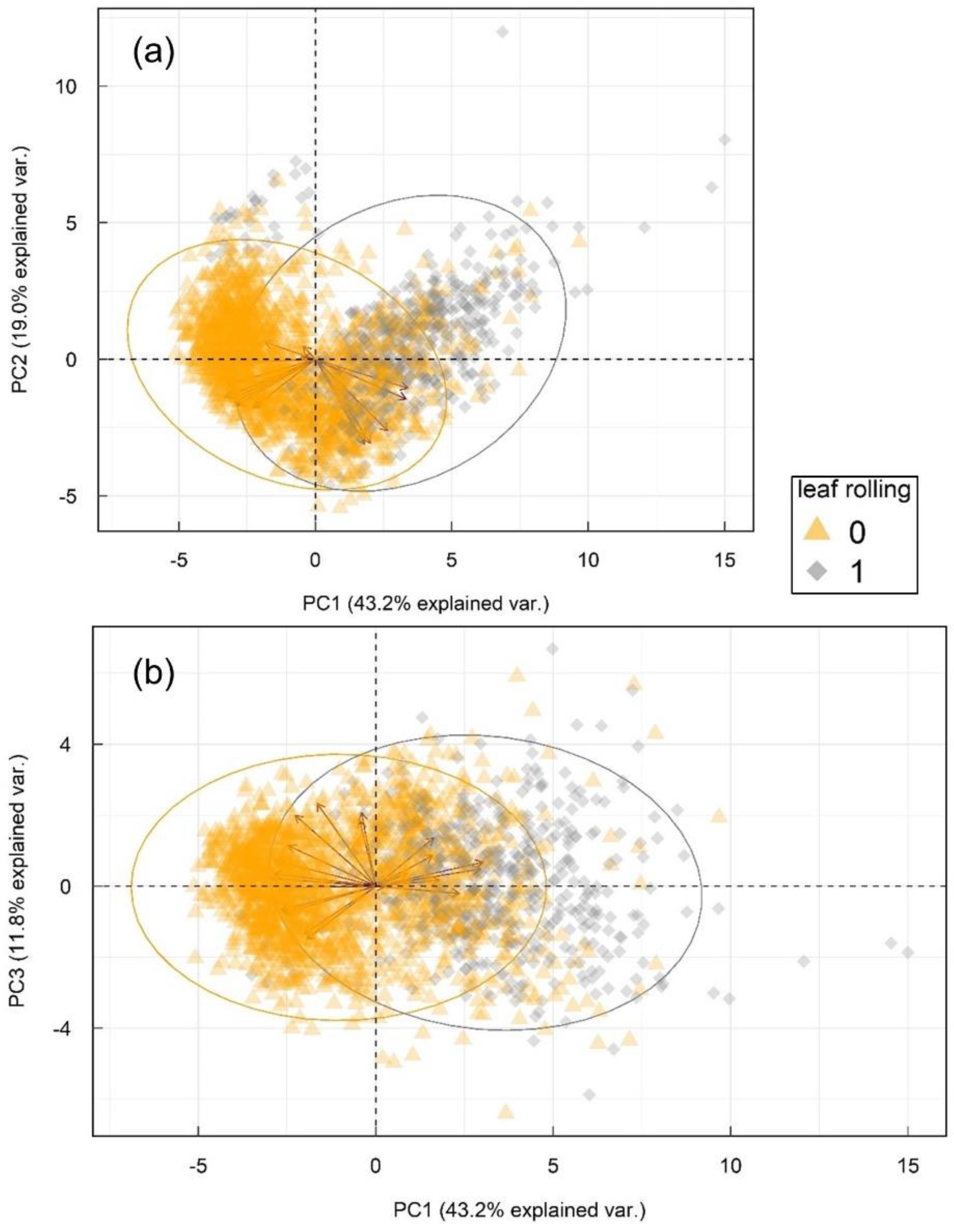
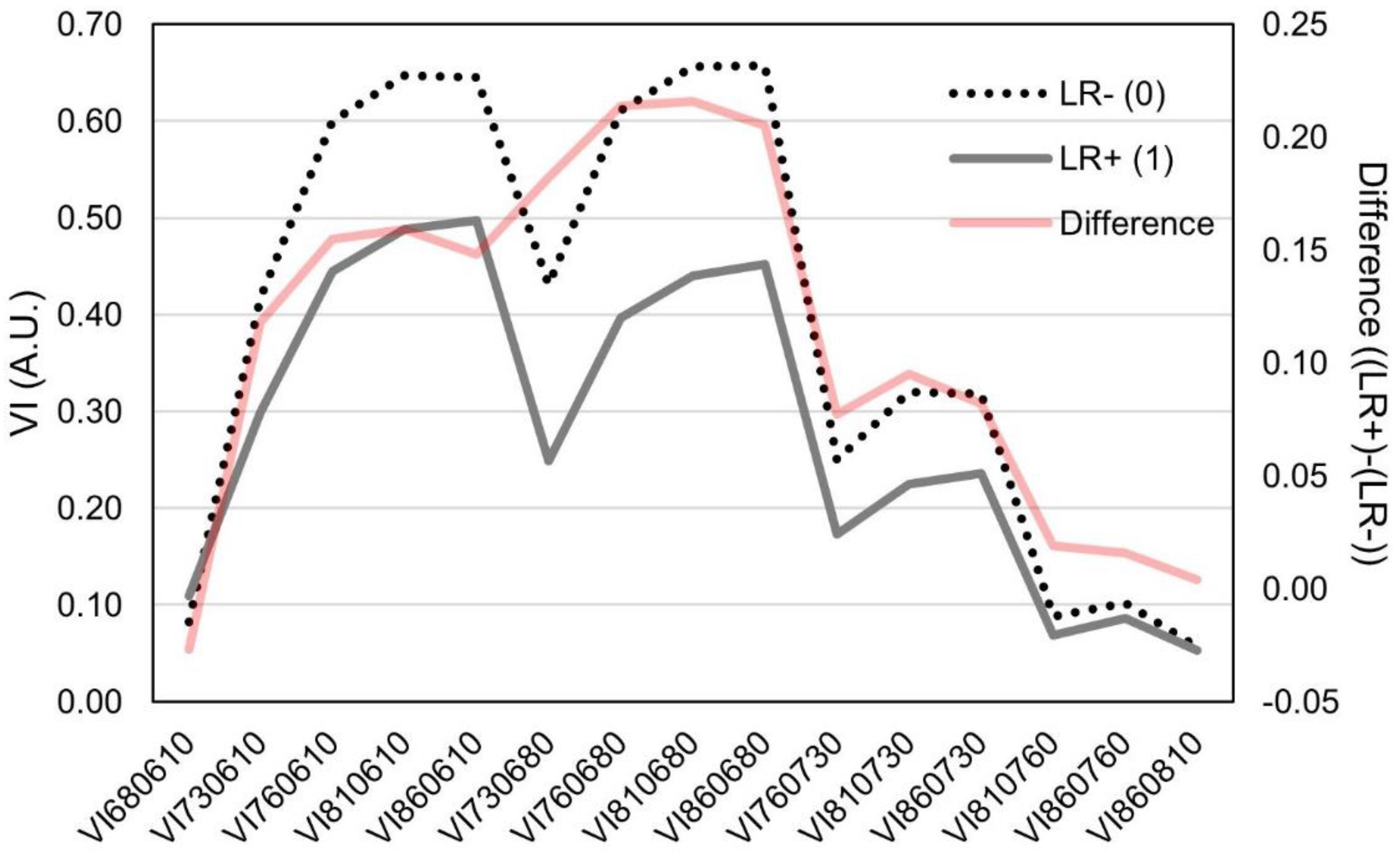
3.1. Changes in Multispectral Sensor Reads in Leaf Rolling Conditions

All measurements in the calibration set were carried out during the extremely dry conditions (Figure S2) and high temperature and VPD (Figure 1a). Conditions changed to very wet when the external validation set was assessed, leading to a low number (7) of plots showing leaf rolling. The analysis of original features showed recognizable patterns of increase/decrease in both calibration (n = 2180) and external (n = 145) datasets showing no leaf rolling (LR−) and leaf rolling (LR+, Table 2). High standard deviations of raw wavelengths indicate the changes in light quality. However, the deviations decreased in VI values reflecting the normalization of the data. Interestingly, all VI values decreased in the LR+ in both datasets except VI680610 which increased slightly in LR+. According to the two-sample t-test, all differences between LR− and LR+ were significant in the calibration set in both original features and Vis. In the external set, significant differences were observed only in reads at 610 and 680 nm among original features. In VIs, a lack of significant differences was observed among all indexes with reads at 730 nm as denominator, and 860 as numerator.
Principal component analysis (Figure 3) showed diverse and substantial correlations between original variables and their projections (PCs), seen as red arrows, e.g., eigenvectors. Full list of loading weights is available online as Table S1. First three principal components explained 74.0% of total variability in the dataset, separate PCs explaining 43.2, 19.0 and 11.8%, respectively. Principal component analysis confirmed patterns from Table 2, rendering two partially overlapping, but separable groups of wavelength changes in leaf rolling conditions in three latent variables. Despite the overlap in part of the responses in lower-dimensional hyperplane (3 PCs), the ability of PCA to capture 74% of variance between groups in only three components with spread in eigenvectors indicates high information density in a small number of underlying features.
Calculation of different normalized vegetation indices represents a convenient mean of auto-normalization of the raw sensor reads. The 15 normalized vegetation indices (termed VI) assessed in this study (Table 2) showed significant variability between leaf rolling and plots without leaf rolling. Interestingly, between wavelengths from the red spectra (610 and 680 nm), lower difference was observed between LR− and LR+ (Figure 4). The same pattern was observed in VIs assessing wavelengths > 700 nm. The largest differences between LR− and LR+ reads were observed in VIs combining wavelengths > 760 nm and <700 nm.

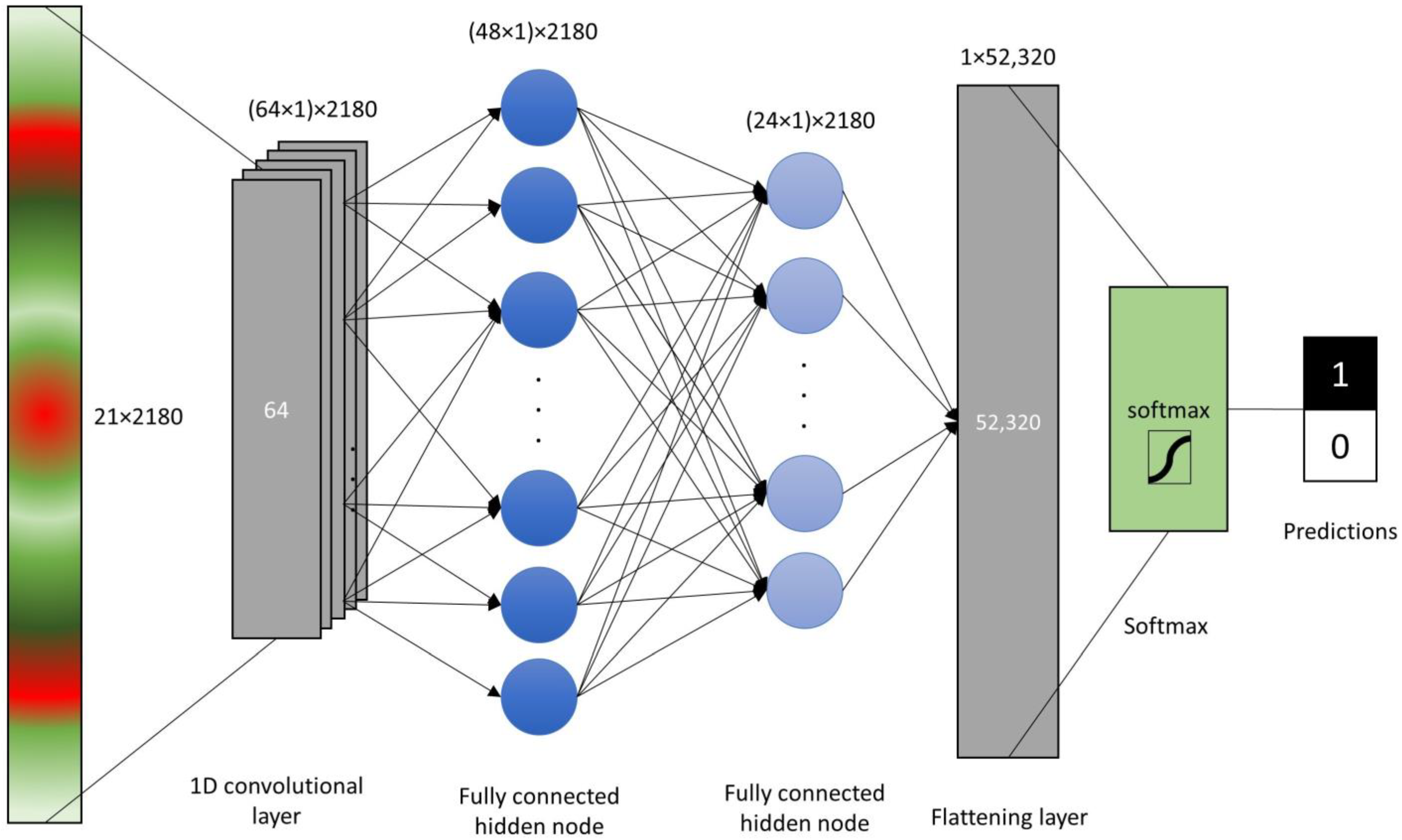
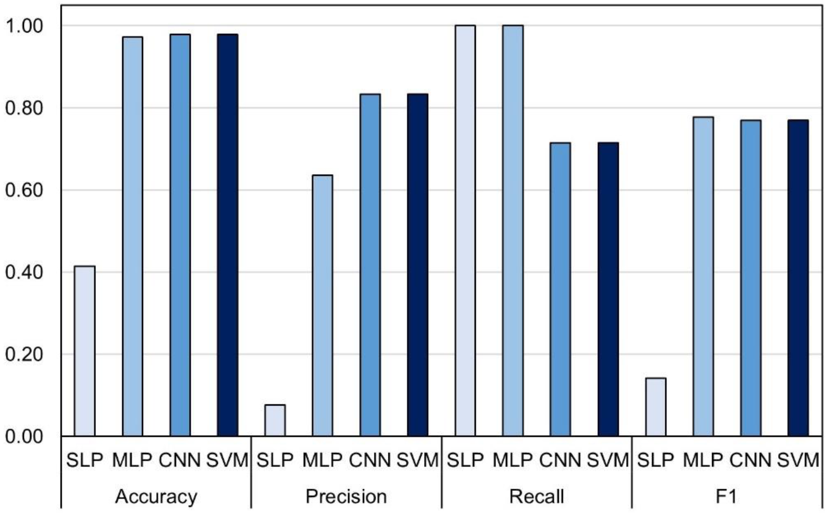
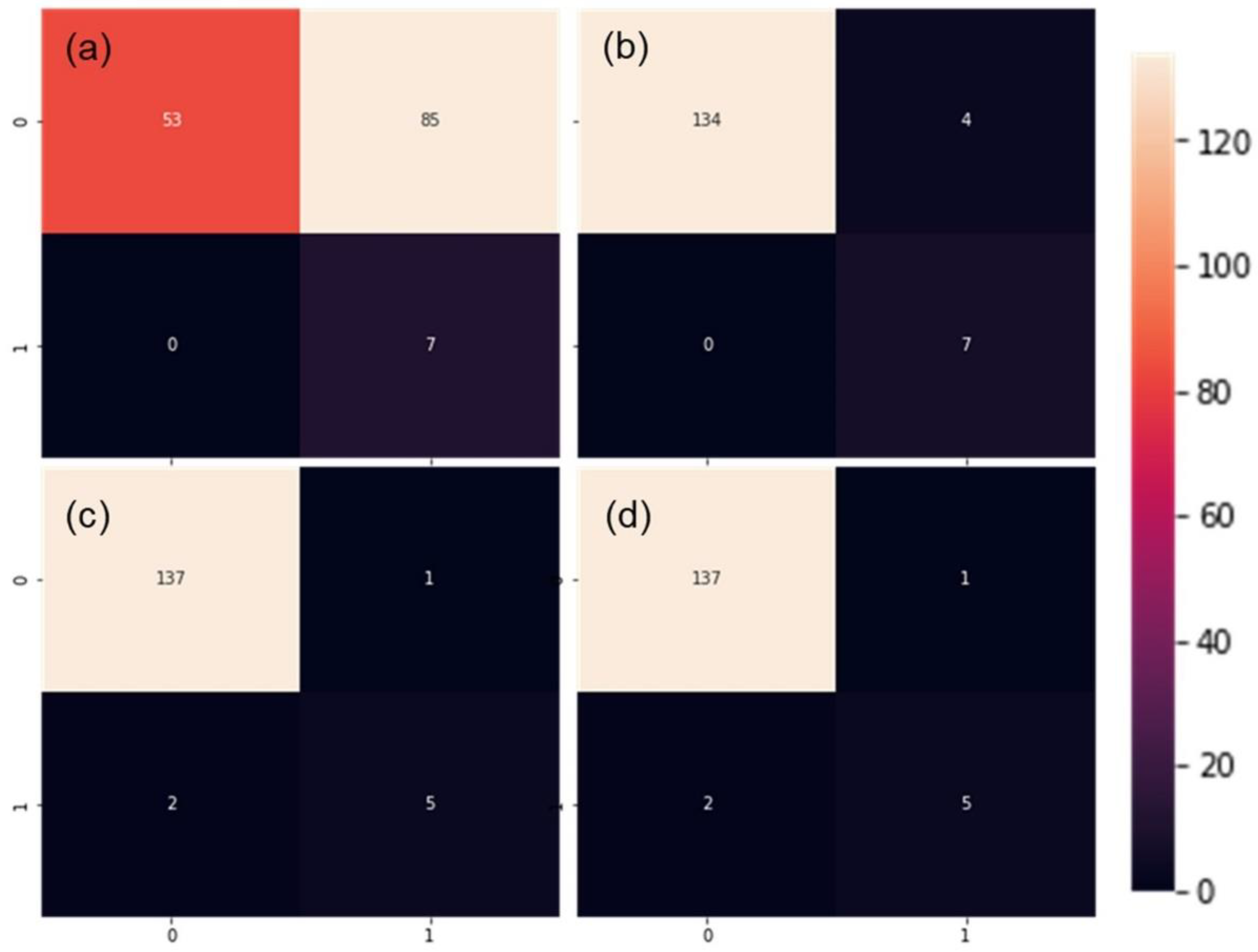
3.2. Assesment Different of Machine Learning Algorithms for Prediction of Leaf Rolling

In stratified 5-fold cross-validation, considerable variability was detected between the performance of different models. Highest prediction accuracy with lowest standard deviation was observed for SLP, followed by CNN, SVM and MLP, respectively (Table 3). Highest precision in cross-validation was observed for SVM, accompanied by second-highest standard deviation between folds. Recall was the highest for SLP, followed by CNN. The highest F1 was observed for CNN. The compute times increased with model complexity in the order SLP < MLP < CNN < SVM. However, when attempting to generalize the results of the calibrated models with the random 15% subset, the prediction accuracies changed. The SLP was shown to be the least accurate model, however, with high recall. According to the precision metrics, the model aimed at target many times (many false positives) which was followed by many hits. Such results indicate overfitting in the model architecture possibly caused by many nodes (128) and only a single layer. Briefly, the model was able to extract features linked to leaf rolling in a stratified set, but when attempting to generalize an unrelated dataset, the performance metrics dramatically decreased.
Support vector machines model showed highest accuracy, but according to the high precision and lowest recall, it was the most conservative model, yielding a low number of false positives. High accuracy and generalization ability of this model is in accordance with results of PCA (Figure 3) and ability of simple dimension reduction (L2 norm in SVC linear kernel) to facilitate efficient feature extraction.
Contrarily, MLP and CNN showed fewer conservative values of precision with second highest accuracy (CNN) and 9.04% lower precision compared to SVM. Multilayer perceptron and CNN showed good generalization ability due to the added layers that mitigated the overfitting found for SLP. The best overall performance was captured by SVM and CNN, with higher accuracy and precision in SVM and higher recall in CNN. This was also confirmed by the highest values of harmonic mean accuracy of the model (F1) which was the highest for CNN, followed by SVM. Overall, compute times for the random subset training and predictions were significantly shorter (10 s to 136 s) compared to the cross-validation procedure.
The performance from validation procedures was mostly in alignment with the test using an external validation dataset. Due to the abundant rain between measurements of calibration and external datasets (Figure 1), there were only seven plots with detectable leaf rolling in the external dataset (Table 2), four of which were detected in SDTrf with sandy loam (not shown). However, this represented an appropriate test of the model robustness, due to the changes in many aspects of plant vitality. Single-layer perceptron maintained poor generalization ability, although with all seven LR+ plots properly classified (Figure 5a).
As in the validation with the random subset, this validation was also followed by a high number of false positives reducing the F1 value to only 14.1 percent (Figure 6) caused by very low precision (7.6%). High number of good classifications (7/7) followed by a relatively conservative number of false positives and no true negatives in MLP (Figure 5b) rewarded the highest F1 score of 77.7% in the external set validation (Figure 6). Marginally lower F1 scores were obtained for CNN and SVM (both 76.9%), which were caused by the inability of the models to correctly classify all seven LR+ plots.

4. Discussion

Phenotyping for drought responses in real time represents a new frontier for crop breeding and precision agriculture [57]; however, the advancements in this field are limited by the high costs of measurement equipment such as unmanned aerial vehicles and hyperspectral cameras. This implies the need for new low-cost proximal or remote sensing solutions, efficiently assessing plant physiological status in real time. Hot and dry conditions during the phenotyping procedure of our study (Figure 1a and Figure S2) in a large number of maize hybrids allowed us to robustly assess a large number of experimental plots with a prototype of multispectral proximal sensing node intended for use in the Internet of Things (IoT) applications. The sensor was used to assess leaf rolling, a trait that was shown to be involved in adaptation to drought and heat conditions [22]. There are various methods for the assessment of leaf rolling [23,29,31,58] and it is well known that different hybrids show different levels of leaf folding, especially given the varying water availability and temperature changes. However, the aim of our work was to assess if the leaf rolling occurrence, despite the varying levels of phenotypic expression, could be spotted or predicted based only on basic reads of spectral responses in red and near-infrared parts of electromagnetic spectra.
At the onset of leaf rolling, many physiological changes take place, such as reduction in photosynthetic activity [59] and changes in metabolic genetic regulatory mechanisms [60]. The reduction in photosynthetic activity should be mostly visible at wavelengths between 710 and 740 nm capturing fluorescence overlap of both photosystem I and II, and 685 nm representing a peak of fluorescence of photosystem II [61] which is within the spectral peaks captured by 680 and 730 nm diodes (according to 20 nm full width at half-maximum) in our study. This was corroborated by the reduction in VIs assessing 680 and 730 nm wavelengths (Table 2, Figure 4).
Stress adaptation, such as the reduction in photochemical activity, also involves translocation of the biochemicals [32]. Additionally, in responses such as leaf rolling, the previously unexposed plant parts become intercepted by sunlight, such as abaxial parts of leaves, having the different pigment mixtures compared to adaxial parts [62]. The reflectance between 700 nm and 980 nm, where the spectral responses of the brown pigments are located, along with chlorophyll fluorescence signals might provide the insight in plant biochemistry, and consequently, physiological status [63]. The exposure of plant abaxial surfaces to sunlight reveals red-brown pigments due to the water deficit [64], thus changing the leaf optical properties [65]. According to the results presented in Weber et al. [66], combined water stress and heat stress, as in our study (Figure 1 and Figure S2), are expected to produce the most visible response in leaf reflectance at wavelengths near the reflectance of brown pigments. This was also confirmed in our results, where the difference between LR− and LR+ increased in indices combining wavelengths > 700 nm and <700 nm (Figure 4). Among these indices is also the commonly used NDVI combining reflectance at approximately 680 and 770 nm [67]. Normalized vegetation indices are traditionally used to assess the vegetation cover from satellite imagery [34], but the advancement of analytic solutions allows their deployment for analysis of a wide range of quantitative and qualitative traits. However, one must note that the usage of multispectral sensor reads also bears the risk of reduced repeatability of the results due to the deviations of atmospheric and sensor effects [68], so the use of VIs is advised, such as Vis in this study.
Due to the rapidly changing climate [69], there is strong pressure on developing new proximal and remote, data-rich high-throughput plant phenotyping solutions, rectified by the lack of manpower and the increased demand for high-quality data [70]. The UAV and phenopole (phenotyping pole) solutions yield similar insight and information density of the reads, however, with more throughput in UAV solutions [71], but more temporal information with phenopoles, facilitating the monitoring of the trait onset dynamics. The sensor node used in our study aims to provide the low-cost solution to this problem, so that the increased density of the sensing nodes, providing the better sampling, could compensate for UAV’s higher throughput, at a lower cost. Furthermore, given the application of our sensor in the envisioned IoT framework, the simultaneous, real-time data collection could provide higher information density compared to UAV, without the need for human intervention [72]. Combining such developments with machine learning methodology should converge to provide new layers of information in plant monitoring paradigm for transition to Agriculture 4.0 [73]. Modelling complex data with unknown hidden features can be efficiently carried out using ML methodology to explain considerable amounts of variance in agricultural production deviations [74]; however, the interpretability of the models is low and despite their high accuracy, they are unable to surrogate the science.
In our study, only marginal differences were observed between MLP, CNN showing good generalization ability due to the added layers that mitigated the overfitting found for SLP. In stratified cross-validation, SLP showed the highest F1 score, followed by the CNN. However, the severe drop in accuracy of SLP in un-stratified datasets can be viewed from the perspective of poor generalization abilities of the networks having a small number of layers with an excessive number of neurons [75], which is apparently the case with SLP presented in our study. Thus, the model was able to extract features linked to leaf rolling in a stratified set, but when attempting to generalize an unrelated dataset, the performance metrics dramatically decreased.
Study on plant Bromus inermis using hyperspectral indices and three ML algorithms, CNN, SVM and random forest, showed feasibility of drought classification in ML framework with the highest prediction accuracies observed for SVM [32]. In our study, SVM also showed the highest overall prediction accuracy in random subset validation. This is also corroborated by the results of PCA (Figure 3) and the ability of a simple dimension reduction technique such as Tikhonov regularization [76] (L2 norm in SVC linear kernel) to facilitate efficient feature extraction.
All models, except SLP, in our study performed well on the given dataset, and the observed differences were not discriminatory. Studies assessing vegetation classifications by the use of hyperspectral imagery with SVM, artificial neural networks and CNN by Hassan et al. [77,78], demonstrating very high classification accuracies reported similar conclusions. The added value in our research can be seen in the analysis of performance in tabular data using additional, unrelated validation dataset (Figure 5 and Figure 6). It was shown that CNN and SVM yielded more conservative, similar performance metrics, while MLP showed the best overall performance, but with only a 1% increase in F1 score. On the other hand, the limitations of our study can be seen from two perspectives. As an early report, our dataset was only created in a single stage of plant development over a limited number of climatological scenarios [79], so further efforts with increased spatial and temporal resolution are needed. Additionally, the deep learning models represent a good way to cope with many types of data taking many conformations in multidimensional hyperplanes, however, with limited interpretability. Further assessment should thus include other ML models such as decision trees retaining more information on the effects of predictor variables.
The usability of ML was also demonstrated at many levels of agricultural production, by using multi/hyperspectral reads and imagery and climatological data, such as disease detection [41,48,80,81,82,83], nutrient deficiency assessment [84,85], stress detection [86,87,88] and in-season predictions of agronomic performance in maize [89,90], sorghum [91], soybean [92], wheat [93,94,95] and cocoa [96]. Corroborating these new avenues in agricultural sciences with the constant involvement of large companies in the development of new learning ML algorithms, and the optimization of the existing ones, Python open-source libraries Tensorflow [97] created and maintained by Google and Pytorch [98] created and maintained by Facebook, makes the future uses of ML incomprehensible.

5. Conclusions

This study demonstrated the ability of machine learning algorithms to use simple multispectral reads for efficient classification of maize leaf rolling. It was shown that there is variability between ML algorithms in terms of performance metrics, but also, computing times. There is a growing need for increased spatiotemporal resolution of plant monitoring with affordable remote sensing solutions, especially in the context of the Internet of Things (IoT). It was demonstrated that ML algorithms can efficiently extract information from multispectral reads and predict plant states such as leaf rolling. Since the envisioned use of the demonstrated sensor is an IoT framework, the inclination is towards less computationally intensive ML algorithms, without sacrificing performance. Thus, the use of MLP might represent the best overall option. Increasing the information density and using smart solutions for decision support in agriculture could facilitate the transition to the Agriculture 4.0 empowered by the nexus between food production and machine learning. Further research should test the framework in multiple topographies and water/nutrient availability scenarios to tackle the abilities of simple and affordable sensing solutions in the dissection of biological systems showing the highest order of complexity.

Supplementary Materials

The following supporting information can be downloaded at: https://www.mdpi.com/article/10.3390/rs14112596/s1, Figure S1. (a) Maize plot showing no leaf rolling (LR−) and a plot with leaf rolling (b); Figure S2. Precipitation during the months of June and July 2021 with 50-year average-based percentiles of dry and wet conditions for Osijek. Gray boxes show measurement times, and the red box shows external validation set measurement time; Figure S3. Learning rates of neural network algorithms from 85% random subset training procedure; Table S1: loading weights of the first three principal components

Author Contributions

Conceptualization, V.G. and J.S.; methodology, V.G. and D.Š.; software, V.G. and J.S.; validation, A.J., J.B. and D.Š.; formal analysis, J.S., J.B., D.Š., and V.G.; field experiments, A.J.; investigation, V.G. and J.S.; resources, A.J., J.B. and D.Š.; data curation, V.G.; writing—original draft preparation, J.S. and V.G.; writing—review and editing, J.B. and D.Š.; visualization, V.G.; funding acquisition, D.Š. All authors have read and agreed to the published version of the manuscript.

Funding

This work is supported by the project “IoT-field: An Ecosystem of Networked Devices and Services for IoT Solutions Applied in Agriculture” co-financed by the European Union from the European Regional Development Fund within the Operational Programme Competitiveness and Cohesion 2014–2020 of the Republic of Croatia.

Data Availability Statement

The data presented in this study are openly available in FigShare at https://doi.org/10.6084/m9.figshare.19904491.v1, reference number 19904491.v1.

Conflicts of Interest

The authors declare no conflict of interest.

References

  1. King, A. The future of agriculture. Nature 2017, 544, S21–S23. [Google Scholar] [CrossRef] [PubMed] [Green Version]
  2. Wang, D.; Cao, W.; Zhang, F.; Li, Z.; Xu, S.; Wu, X. A Review of Deep Learning in Multiscale Agricultural Sensing. Remote Sens. 2022, 14, 559. [Google Scholar] [CrossRef]
  3. Polpanich, O.; Bhatpuria, D.; Fernanda, T.; Santos, S. Leveraging Multi-Source Data and Digital Technology to Support the Monitoring of Localized Water Changes in the Mekong Region; SEI: Oaks, PA, USA, 2022. [Google Scholar]
  4. Trnka, M.; Hlavinka, P.; Možný, M.; Semerádová, D.; Štěpánek, P.; Balek, J.; Bartošová, L.; Zahradníček, P.; Bláhová, M.; Skalák, P.; et al. Czech Drought Monitor System for monitoring and forecasting agricultural drought and drought impacts. Int. J. Climatol. 2020, 40, 5941–5958. [Google Scholar] [CrossRef]
  5. Johnson, L.F.; Trout, T.J. Satellite NDVI assisted monitoring of vegetable crop evapotranspiration in california’s san Joaquin Valley. Remote Sens. 2012, 4, 439–455. [Google Scholar] [CrossRef] [Green Version]
  6. Takeuchi, W.; Darmawan, S.; Shofiyati, R.; Khiem, M.V.; Oo, K.S.; Pimple, U.; Heng, S. Near-real time meteorological drought monitoring and early warning system for croplands in Asia. In Proceedings of the ACRS 2015: The 36th Asian Conference on Remote Sensing “Fostering Resilient Growth in Asia”, Quezon City, Philippines, 19–23 October 2015; pp. 171–178. [Google Scholar]
  7. Minamiguchi, N. The application of geospatial and disaster information for food insecurity and agricultural drought monitoring and assessment by the FAO GIEWS and Asia FIVIMS. Work. Reducing Food Insecurity Assoc. 2005, 27, 28. [Google Scholar]
  8. Zhang, Y.; Han, W.; Niu, X.; Li, G. Maize crop coefficient estimated from UAV-measured multispectral vegetation indices. Sensors 2019, 19, 5250. [Google Scholar] [CrossRef] [Green Version]
  9. Ramos-Giraldo, P.; Reberg-Horton, C.; Locke, A.M.; Mirsky, S.; Lobaton, E. Drought Stress Detection Using Low-Cost Computer Vision Systems and Machine Learning Techniques. IT Prof. 2020, 22, 27–29. [Google Scholar] [CrossRef]
  10. dos Santos, R.A.; Mantovani, E.C.; Filgueiras, R.; Fernandes-Filho, E.I.; da Silva, A.C.B.; Venancio, L.P. Actual evapotranspiration and biomass of maize from a red-green-near-infrared (RGNIR) sensor on board an unmanned aerial vehicle (UAV). Water 2020, 12, 1–20. [Google Scholar]
  11. Du, S.; Liu, L.; Liu, X.; Guo, J.; Hu, J.; Wang, S.; Zhang, Y. SIFSpec: Measuring solar-induced chlorophyll fluorescence observations for remote sensing of photosynthesis. Sensors 2019, 19, 3009. [Google Scholar] [CrossRef] [Green Version]
  12. Zhang, Y.; Zhang, Q.; Liu, L.; Zhang, Y.; Wang, S.; Ju, W.; Zhou, G.; Zhou, L.; Tang, J.; Zhu, X.; et al. ChinaSpec: A Network for Long-Term Ground-Based Measurements of Solar-Induced Fluorescence in China. J. Geophys. Res. Biogeosci. 2021, 126, e2020JG006042. [Google Scholar] [CrossRef]
  13. Lhotka, O.; Kyselý, J.; Farda, A. Climate change scenarios of heat waves in Central Europe and their uncertainties. Theor. Appl. Climatol. 2018, 131, 1043–1054. [Google Scholar] [CrossRef]
  14. Lobell, D.B.; Roberts, M.J.; Schlenker, W.; Braun, N.; Little, B.B.; Rejesus, R.M.; Hammer, G.L. Greater sensitivity to drought accompanies maize yield increase in the U.S. Midwest. Science 2014, 344, 516–519. [Google Scholar] [CrossRef] [PubMed]
  15. Sah, R.P.; Chakraborty, M.; Prasad, K.; Pandit, M.; Tudu, V.K.; Chakravarty, M.K.; Narayan, S.C.; Rana, M.; Moharana, D. Impact of water deficit stress in maize: Phenology and yield components. Sci. Rep. 2020, 10, 2944. [Google Scholar] [CrossRef] [PubMed]
  16. Harrison, M.T.; Tardieu, F.; Dong, Z.; Messina, C.D.; Hammer, G.L. Characterizing drought stress and trait influence on maize yield under current and future conditions. Glob. Chang. Biol. 2014, 20, 867–878. [Google Scholar] [CrossRef]
  17. Ribaut, J.; Betran, J.; Monneveux, P.; Setter, T. Drought Tolerance in Maize. In Handbook of Maize: Its Biology; Bennetzen, J.L., Hake, S., Eds.; Springer Science + Business Media, LLC: Berlin, Germany, 2009; ISBN 9780387794181. [Google Scholar]
  18. Aslam, M.; Maqbool, M.A.; Cengiz, R. Drought Stress in Maize (Zea mays L.); Springer: Berlin, Germany, 2015; ISBN 978-3-319-25440-1. [Google Scholar]
  19. Masuka, B.; Araus, J.L.; Das, B.; Sonder, K.; Cairns, J.E. Phenotyping for Abiotic Stress Tolerance in Maize. J. Integr. Plant Biol. 2012, 54, 238–249. [Google Scholar] [CrossRef]
  20. Beebe, S.E.; Rao, I.M.; Blair, M.W.; Acosta-Gallegos, J.A. Phenotyping common beans for adaptation to drought. Front. Physiol. 2013, 4, 35. [Google Scholar] [CrossRef] [Green Version]
  21. Moulia, B. Leaves as shell structures: Double curvature, auto-stresses, and minimal mechanical energy constraints on leaf rolling in grasses. J. Plant Growth Regul. 2000, 19, 19–30. [Google Scholar] [CrossRef]
  22. Monneveux, P.; Sanchez, C.; Tiessen, A. Future progress in drought tolerance in maize needs new secondary traits and cross combinations. J. Agric. Sci. 2008, 146, 287–300. [Google Scholar] [CrossRef] [Green Version]
  23. Gao, L.; Yang, G.; Li, Y.; Fan, N.; Li, H.; Zhang, M.; Xu, R.; Zhang, M.; Zhao, A.; Ni, Z.; et al. Fine mapping and candidate gene analysis of a QTL associated with leaf rolling index on chromosome 4 of maize (Zea mays L.). Theor. Appl. Genet. 2019, 132, 3047–3062. [Google Scholar] [CrossRef]
  24. Sirault, X.R.R.; Condon, A.G.; Wood, J.T.; Farquhar, G.D.; Rebetzke, G.J. “Rolled-upness”: Phenotyping leaf rolling in cereals using computer vision and functional data analysis approaches. Plant Methods 2015, 11, 52. [Google Scholar] [CrossRef] [Green Version]
  25. Fernandez, D.; Castrillo, M. Maize Leaf Roling Initiation. Photosynthetica 1999, 37, 493–497. [Google Scholar] [CrossRef]
  26. Cal, A.J.; Sanciangco, M.; Rebolledo, M.C.; Luquet, D.; Torres, R.O.; McNally, K.L.; Henry, A. Leaf morphology, rather than plant water status, underlies genetic variation of rice leaf rolling under drought. Plant Cell Environ. 2019, 42, 1532–1544. [Google Scholar] [CrossRef] [PubMed] [Green Version]
  27. Kenchanmane Raju, S.K.; Adkins, M.; Enersen, A.; Santana de Carvalho, D.; Studer, A.J.; Ganapathysubramanian, B.; Schnable, P.S.; Schnable, J.C. Leaf Angle eXtractor: A high-throughput image processing framework for leaf angle measurements in maize and sorghum. Appl. Plant Sci. 2020, 8, 1–9. [Google Scholar] [CrossRef] [PubMed]
  28. O’Toole, J.C.; Cruz, R.T.; Singh, T.N. Leaf rolling and transpiration. Plant Sci. Lett. 1979, 16, 111–114. [Google Scholar] [CrossRef]
  29. Premachandra, G.S.; Saneoka, H.; Fujita, K.; Ogata, S. Water Stress and Potassium Fertilization in Field Grown Maize (Zea mays L.): Effects on Leaf Water Relations and Leaf Rolling. J. Agron. Crop Sci. 1993, 170, 195–201. [Google Scholar] [CrossRef]
  30. Bolaños, J.; Edmeades, G.O. The importance of the anthesis-silking interval in breeding for drought tolerance in tropical maize. F. Crop. Res. 1996, 48, 65–80. [Google Scholar] [CrossRef]
  31. Baret, F.; Madec, S.; Irfan, K.; Lopez, J.; Comar, A.; Hemmerlé, M.; Dutartre, D.; Praud, S.; Tixier, M.H. Leaf-rolling in maize crops: From leaf scoring to canopy-level measurements for phenotyping. J. Exp. Bot. 2018, 69, 2705–2716. [Google Scholar] [CrossRef] [PubMed]
  32. Dao, P.D.; He, Y.; Proctor, C. Plant drought impact detection using ultra-high spatial resolution hyperspectral images and machine learning. Int. J. Appl. Earth Obs. Geoinf. 2021, 102, 102364. [Google Scholar] [CrossRef]
  33. Calderón, R.; Navas-Cortés, J.A.; Lucena, C.; Zarco-Tejada, P.J. High-resolution airborne hyperspectral and thermal imagery for early detection of Verticillium wilt of olive using fluorescence, temperature and narrow-band spectral indices. Remote Sens. Environ. 2013, 139, 231–245. [Google Scholar] [CrossRef]
  34. Xue, J.; Su, B. Significant remote sensing vegetation indices: A review of developments and applications. J. Sens. 2017, 2017, 1353691. [Google Scholar] [CrossRef] [Green Version]
  35. Dmitriev, P.A.; Kozlovsky, B.L.; Kupriushkin, D.P.; Lysenko, V.S.; Rajput, V.D.; Ignatova, M.A.; Tarik, E.P.; Kapralova, O.A.; Tokhtar, V.K.; Singh, A.K.; et al. Identification of species of the genus Acer L. using vegetation indices calculated from the hyperspectral images of leaves. Remote Sens. Appl. Soc. Environ. 2022, 25, 100679. [Google Scholar] [CrossRef]
  36. Zarco-Tejada, P.J.; González-Dugo, V.; Berni, J.A.J. Fluorescence, temperature and narrow-band indices acquired from a UAV platform for water stress detection using a micro-hyperspectral imager and a thermal camera. Remote Sens. Environ. 2012, 117, 322–337. [Google Scholar] [CrossRef]
  37. Mohammed, G.H.; Colombo, R.; Middleton, E.M.; Rascher, U.; van der Tol, C.; Nedbal, L.; Goulas, Y.; Pérez-Priego, O.; Damm, A.; Meroni, M.; et al. Remote sensing of solar-induced chlorophyll fluorescence (SIF) in vegetation: 50 years of progress. Remote Sens. Environ. 2019, 231, 111177. [Google Scholar] [CrossRef] [PubMed]
  38. Virnodkar, S.S.; Pachghare, V.K.; Patil, V.C.; Jha, S.K. Remote Sensing and Machine Learning for Crop Water Stress Determination in Various Crops: A Critical Review. Precis. Agric. 2020, 21, 1121–1155. [Google Scholar]
  39. Niazian, M.; Niedbała, G. Machine learning for plant breeding and biotechnology. Agriculture 2020, 10, 436. [Google Scholar] [CrossRef]
  40. Singh, A.; Ganapathysubramanian, B.; Singh, A.K.; Sarkar, S. Machine Learning for High-Throughput Stress Phenotyping in Plants. Trends Plant Sci. 2016, 21, 110–124. [Google Scholar] [CrossRef] [Green Version]
  41. Behmann, J.; Mahlein, A.K.; Rumpf, T.; Römer, C.; Plümer, L. A review of advanced machine learning methods for the detection of biotic stress in precision crop protection. Precis. Agric. 2015, 16, 239–260. [Google Scholar] [CrossRef]
  42. Barradas, A.; Correia, P.M.P.; Silva, S.; Mariano, P.; Pires, M.C.; Matos, A.R.; da Silva, A.B.; Marques da Silva, J. Comparing machine learning methods for classifying plant drought stress from leaf reflectance spectra in arabidopsis thaliana. Appl. Sci. 2021, 11, 6392. [Google Scholar] [CrossRef]
  43. Feng, X.; Zhan, Y.; Wang, Q.; Yang, X.; Yu, C.; Wang, H.; Tang, Z.Y.; Jiang, D.; Peng, C.; He, Y. Hyperspectral imaging combined with machine learning as a tool to obtain high-throughput plant salt-stress phenotyping. Plant J. 2020, 101, 1448–1461. [Google Scholar] [CrossRef]
  44. Verrelst, J.; Camps-Valls, G.; Muñoz-Marí, J.; Rivera, J.P.; Veroustraete, F.; Clevers, J.G.P.W.; Moreno, J. Optical remote sensing and the retrieval of terrestrial vegetation bio-geophysical properties—A review. ISPRS J. Photogramm. Remote Sens. 2015, 108, 273–290. [Google Scholar] [CrossRef]
  45. Zhang, L.; Peng, L.; Zhang, T.; Cao, S.; Peng, Z. Infrared small target detection via non-convex rank approximation minimization joint l2,1 norm. Remote Sens. 2018, 10, 1821. [Google Scholar] [CrossRef] [Green Version]
  46. Maxwell, A.E.; Warner, T.A.; Fang, F. Implementation of machine-learning classification in remote sensing: An applied review. Int. J. Remote Sens. 2018, 39, 2784–2817. [Google Scholar] [CrossRef] [Green Version]
  47. Ali, I.; Greifeneder, F.; Stamenkovic, J.; Neumann, M.; Notarnicola, C. Review of machine learning approaches for biomass and soil moisture retrievals from remote sensing data. Remote Sens. 2015, 7, 16398–16421. [Google Scholar] [CrossRef] [Green Version]
  48. Zheng, C.; Abd-elrahman, A.; Whitaker, V. Remote sensing and machine learning in crop phenotyping and management, with an emphasis on applications in strawberry farming. Remote Sens. 2021, 13, 531. [Google Scholar] [CrossRef]
  49. Zhao, R.; Li, Y.; Ma, M. Mapping paddy rice with satellite remote sensing: A review. Sustainability 2021, 13, 503. [Google Scholar] [CrossRef]
  50. Kattenborn, T.; Leitloff, J.; Schiefer, F.; Hinz, S. Review on Convolutional Neural Networks (CNN) in vegetation remote sensing. ISPRS J. Photogramm. Remote Sens. 2021, 173, 24–49. [Google Scholar] [CrossRef]
  51. Holloway, J.; Mengersen, K. Statistical machine learning methods and remote sensing for sustainable development goals: A review. Remote Sens. 2018, 10, 1365. [Google Scholar] [CrossRef] [Green Version]
  52. Mitter, H.; Techen, A.K.; Sinabell, F.; Helming, K.; Schmid, E.; Bodirsky, B.L.; Holman, I.; Kok, K.; Lehtonen, H.; Leip, A.; et al. Shared Socio-economic Pathways for European agriculture and food systems: The Eur-Agri-SSPs. Glob. Environ. Chang. 2020, 65, 102159. [Google Scholar] [CrossRef]
  53. Dwyer, L.M.; Stewart, D.W.; Carrigan, L.; Ma, B.L.; Neave, P.; Balchin, D. Guidelines for comparisons among different maize maturity. Agron. J. 1999, 91, 946–949. [Google Scholar] [CrossRef]
  54. Araus, J.L.; Serret, M.D.; Edmeades, G.O. Phenotyping maize for adaptation to drought. Front. Physiol. 2012, 3, 305. [Google Scholar] [CrossRef] [Green Version]
  55. Liu, X.; Wang, X.; Wang, X.; Gao, J.; Luo, N.; Meng, Q.; Wang, P. Dissecting the critical stage in the response of maize kernel set to individual and combined drought and heat stress around flowering. Environ. Exp. Bot. 2020, 179, 104213. [Google Scholar] [CrossRef]
  56. R Core Team. R: A Language and Environment for Statistical Computing; R Foundation for Statistical Computing: Vienna, Austria, 2021. [Google Scholar]
  57. Araus, J.L.; Cairns, J.E. Field high-throughput phenotyping: The new crop breeding frontier. Trends Plant Sci. 2014, 19, 52–61. [Google Scholar] [CrossRef] [PubMed]
  58. Saruhan, N.; Saglam, A.; Kadioglu, A. Salicylic acid pretreatment induces drought tolerance and delays leaf rolling by inducing antioxidant systems in maize genotypes. Acta Physiol. Plant. 2012, 34, 97–106. [Google Scholar] [CrossRef]
  59. Saglam, A.; Kadioglu, A.; Demiralay, M.; Terzi, R. Leaf rolling reduces photosynthetic loss in maize under severe drought. Acta Bot. Croat. 2014, 73, 315–332. [Google Scholar] [CrossRef]
  60. Kadioglu, A.; Terzi, R.; Saruhan, N.; Saglam, A. Current advances in the investigation of leaf rolling caused by biotic and abiotic stress factors. Plant Sci. 2012, 182, 42–48. [Google Scholar] [CrossRef]
  61. Kim, E.; Ahn, T.K.; Kumazaki, S. Changes in antenna sizes of photosystems during state transitions in granal and stroma-exposed thylakoid membrane of intact chloroplasts in arabidopsis mesophyll protoplasts. Plant Cell Physiol. 2015, 56, 759–768. [Google Scholar] [CrossRef] [Green Version]
  62. Lu, Z.; Quiñones, M.A.; Zeiger, E. Abaxial and adaxial stomata from Pima cotton (Gossypium barbadense L.) differ in their pigment content and sensitivity to light quality. Plant. Cell Environ. 1993, 16, 851–858. [Google Scholar] [CrossRef]
  63. Peñuelas, J.; Filella, L. Technical focus: Visible and near-infrared reflectance techniques for diagnosing plant physiological status. Trends Plant Sci. 1998, 3, 151–156. [Google Scholar] [CrossRef]
  64. Moore, J.P.; Hearshaw, M.; Ravenscroft, N.; Lindsey, G.G.; Farrant, J.M.; Brandt, W.F. Desiccation-induced ultrastructural and biochemical changes in the leaves of the resurrection plant Myrothamnus flabellifolia. Aust. J. Bot. 2007, 55, 482–491. [Google Scholar] [CrossRef]
  65. Hughes, N.M.; Vogelmann, T.C.; Smith, W.K. Optical effects of abaxial anthocyanin on absorption of red wavelengths by understorey species: Revisiting the back-scatter hypothesis. J. Exp. Bot. 2008, 59, 3435–3442. [Google Scholar] [CrossRef]
  66. Weber, V.S.; Araus, J.L.; Cairns, J.E.; Sanchez, C.; Melchinger, A.E.; Orsini, E. Prediction of grain yield using reflectance spectra of canopy and leaves in maize plants grown under different water regimes. F. Crop. Res. 2012, 128, 82–90. [Google Scholar] [CrossRef]
  67. Martin, D.E.; López, J.D.; Lan, Y. Laboratory evaluation of the GreenSeekerTM hand-held optical sensor to variations in orientation and height above canopy. Int. J. Agric. Biol. Eng. 2012, 5, 43–47. [Google Scholar]
  68. Huang, S.; Tang, L.; Hupy, J.P.; Wang, Y.; Shao, G. A commentary review on the use of normalized difference vegetation index (NDVI) in the era of popular remote sensing. J. For. Res. 2021, 32, 1–6. [Google Scholar] [CrossRef]
  69. Dietz, K.J.; Zörb, C.; Geilfus, C.M. Drought and crop yield. Plant Biol. 2021, 23, 881–893. [Google Scholar] [CrossRef] [PubMed]
  70. Reynolds, D.; Baret, F.; Welcker, C.; Bostrom, A.; Ball, J.; Cellini, F.; Lorence, A.; Chawade, A.; Khafif, M.; Noshita, K.; et al. What is cost-efficient phenotyping? Optimizing costs for different scenarios. Plant Sci. 2019, 282, 14–22. [Google Scholar] [CrossRef] [Green Version]
  71. Gracia-Romero, A.; Kefauver, S.C.; Vergara-Díaz, O.; Hamadziripi, E.; Zaman-Allah, M.A.; Thierfelder, C.; Prassana, B.M.; Cairns, J.E.; Araus, J.L. Leaf versus whole-canopy remote sensing methodologies for crop monitoring under conservation agriculture: A case of study with maize in Zimbabwe. Sci. Rep. 2020, 10, 16008. [Google Scholar] [CrossRef]
  72. Sun, D.; Robbins, K.; Morales, N.; Shu, Q.; Cen, H. Advances in optical phenotyping of cereal crops. Trends Plant Sci. 2022, 27, 191–208. [Google Scholar] [CrossRef]
  73. Herrmann, I.; Berger, K. Remote and proximal assessment of plant traits. Remote Sens. 2021, 13, 1893. [Google Scholar] [CrossRef]
  74. Lischeid, G.; Webber, H.; Sommer, M.; Nendel, C.; Ewert, F. Machine learning in crop yield modelling: A powerful tool, but no surrogate for science. Agric. For. Meteorol. 2022, 312, 108698. [Google Scholar] [CrossRef]
  75. Hunter, D.; Yu, H.; Pukish, M.S.; Kolbusz, J.; Wilamowski, B.M. Selection of proper neural network sizes and architectures-A comparative study. IEEE Trans. Ind. Inform. 2012, 8, 228–240. [Google Scholar] [CrossRef]
  76. Tikhonov, A.N.; Arsenin, V.Y. Solutions of Ill-Posed Problems; John Wiley & Sons: New York, NY, USA, 1977. [Google Scholar]
  77. Hasan, H.; Shafri, H.Z.M.; Habshi, M. A Comparison between Support Vector Machine (SVM) and Convolutional Neural Network (CNN) Models for Hyperspectral Image Classification. IOP Conf. Ser. Earth Environ. Sci. 2019, 357, 012035. [Google Scholar] [CrossRef] [Green Version]
  78. Hasan, M.; Ullah, S.; Khan, M.J.; Khurshid, K. Comparative analysis of SVM, ann and cnn for classifying vegetation species using hyperspectral thermal infrared data. Int. Arch. Photogramm. Remote Sens. Spat. Inf. Sci.—ISPRS Arch. 2019, 42, 1861–1868. [Google Scholar] [CrossRef] [Green Version]
  79. Galic, V.; Franic, M.; Jambrovic, A.; Ledencan, T.; Brkic, A.; Zdunic, Z.; Simic, D. Genetic correlations between photosynthetic and yield performance in maize are different under two heat scenarios during flowering. Front. Plant Sci. 2019, 10, 566. [Google Scholar] [CrossRef] [PubMed]
  80. Odilbekov, F.; Armoniené, R.; Henriksson, T.; Chawade, A. Proximal phenotyping and machine learning methods to identify septoria tritici blotch disease symptoms in wheat. Front. Plant Sci. 2018, 9, 1–11. [Google Scholar] [CrossRef]
  81. Appeltans, S.; Pieters, J.G.; Mouazen, A.M. Detection of leek rust disease under field conditions using hyperspectral proximal sensing and machine learning. Remote Sens. 2021, 13, 1341. [Google Scholar] [CrossRef]
  82. Ouhami, M.; Hafiane, A.; Es-Saady, Y.; El Hajji, M.; Canals, R. Computer Vision, IoT and Data Fusion for Crop Disease Detection Using Machine Learning: A Survey and Ongoing Research. Remote Sens. 2021, 13, 2486. [Google Scholar] [CrossRef]
  83. Esposito, S.; Carputo, D.; Cardi, T.; Tripodi, P. Applications and Trends of Machine Learning in Genomics and Phenomics for Next-Generation Breeding. Plants 2020, 9, 34. [Google Scholar] [CrossRef] [Green Version]
  84. Barbedo, J.G.A. Detection of nutrition deficiencies in plants using proximal images and machine learning: A review. Comput. Electron. Agric. 2019, 162, 482–492. [Google Scholar] [CrossRef]
  85. Li, D.; Miao, Y.; Ransom, C.J.; Bean, G.M.; Kitchen, N.R.; Fernández, F.G.; Sawyer, J.E.; Camberato, J.J.; Carter, P.R.; Ferguson, R.B.; et al. Corn Nitrogen Nutrition Index Prediction Improved by Integrating Genetic, Environmental, and Management Factors with Active Canopy Sensing Using Machine Learning. Remote Sens. 2022, 14, 394. [Google Scholar] [CrossRef]
  86. Zubler, A.V.; Yoon, J.Y. Proximal Methods for Plant Stress Detection Using Optical Sensors and Machine Learning. Biosensors 2020, 10, 193. [Google Scholar] [CrossRef]
  87. Kumar, D.; Kushwaha, S.; Delvento, C.; Liatukas, Ž.; Chawade, A. Affordable Phenotyping of Winter Wheat under Field and Controlled Conditions for Drought Tolerance. Agronomy 2020, 10, 882. [Google Scholar] [CrossRef]
  88. Deery, D.; Jimenez-Berni, J.; Jones, H.; Sirault, X.; Furbank, R. Proximal Remote Sensing Buggies and Potential Applications for Field-Based Phenotyping. Agronomy 2014, 4, 349–379. [Google Scholar] [CrossRef] [Green Version]
  89. Mupangwa, W.; Chipindu, L.; Nyagumbo, I.; Mkuhlani, S.; Sisito, G. Evaluating machine learning algorithms for predicting maize yield under conservation agriculture in Eastern and Southern Africa. SN Appl. Sci. 2020, 2, 1–14. [Google Scholar] [CrossRef]
  90. Yang, W.; Nigon, T.; Hao, Z.; Dias Paiao, G.; Fernández, F.G.; Mulla, D.; Yang, C. Estimation of corn yield based on hyperspectral imagery and convolutional neural network. Comput. Electron. Agric. 2021, 184, 106092. [Google Scholar] [CrossRef]
  91. Habyarimana, E.; Baloch, F.S. Machine learning models based on remote and proximal sensing as potential methods for in-season biomass yields prediction in commercial sorghum fields. PLoS ONE 2021, 16, 1–23. [Google Scholar] [CrossRef]
  92. Teodoro, P.E.; Teodoro, L.P.R.; Baio, F.H.R.; da Silva Junior, C.A.; Dos Santos, R.G.; Ramos, A.P.M.; Pinheiro, M.M.F.; Osco, L.P.; Gonçalves, W.N.; Carneiro, A.M.; et al. Predicting Days to Maturity, Plant Height, and Grain Yield in Soybean: A Machine and Deep Learning Approach Using Multispectral Data. Remote Sens. 2021, 13, 4632. [Google Scholar] [CrossRef]
  93. Wang, X.; Huang, J.; Feng, Q.; Yin, D. Winter wheat yield prediction at county level and uncertainty analysis in main wheat-producing regions of China with deep learning approaches. Remote Sens. 2020, 12, 1744. [Google Scholar] [CrossRef]
  94. Peichl, M.; Thober, S.; Samaniego, L.; Hansjürgens, B.; Marx, A. Machine-learning methods to assess the effects of a non-linear damage spectrum taking into account soil moisture on winter wheat yields in Germany. Hydrol. Earth Syst. Sci. 2021, 25, 6523–6545. [Google Scholar] [CrossRef]
  95. Guberac, S.; Galić, V.; Rebekić, A.; Čupić, T.; Petrović, S. Optimising accuracy of performance predictions using available morphophysiological information in wheat breeding germplasm. Ann. Appl. Biol. 2021, 178, 367–376. [Google Scholar] [CrossRef]
  96. Lamos-Díaz, H.; Puentes-Garzón, D.E.; Zarate-Caicedo, D.A. Comparison between Machine Learning Models for Yield Forecast in Cocoa Crops in Santander, Colombia. Rev. Fac. Ing. 2020, 29, e10853. [Google Scholar] [CrossRef]
  97. Abadi, M.; Barham, P.; Chen, J.; Chen, Z.; Davis, A.; Dean, J.; Devin, M.; Ghemawat, S.; Irving, G.; Isard, M.; et al. TensorFlow: A system for large-scale machine learning. In Proceedings of the 12th USENIX Symposium on Operating Systems Design and Implementation (OSDI 16), Savannah, GA, USA, 2–4 November 2016. [Google Scholar]
  98. Paszke, A.; Gross, S.; Massa, F.; Lerer, A.; Bradbury Google, J.; Chanan, G.; Killeen, T.; Lin, Z.; Gimelshein, N.; Antiga, L.; et al. PyTorch: An Imperative Style, High-Performance Deep Learning Library. arXiv 2019, arXiv:1912.01703. [Google Scholar]
Figure 1. Schematic representation of measurement process. (a) shows diurnal temperatures (°C), vapor pressure deficit (hPa) and daily precipitation (mm/m2) for July 2021. Gray boxes show measurement times, and the red box shows external validation set measurement time. (b) shows the position of tripod mounted sensor in plant stands, and (c) is a tripod mounted sensor wiring used to carry out the measurements. In (c), left image represents the tripod-mounted unit, in the middle is a close-up of wiring and a printed mount, while the right image shows AMS AS7263 sensor unit on a breakout board.
Remotesensing 14 02596 g001
Figure 2. Schematic representation of the convolutional neural network (CNN) with single convolution layer, 2 hidden fully connected nodes, flattening layer and a softmax function.
Remotesensing 14 02596 g002
Figure 3. Principal component analysis of the multispectral sensor reads and the corresponding normalized difference vegetation indexes. (a) shows principal components 1 and 2, and principal components 1 and 3 are shown in (b). Arrows represent eigenvectors of the variables (Table S1) and ellipses represent 95% confidence intervals for each group based on Gaussian distribution.
Remotesensing 14 02596 g003
Figure 4. Plot of different normalized difference vegetation indices (VI) in arbitrary units (A.U.) between plots showing leaf rolling (LR+) and plots without leaf rolling (LR−) and their respective differences. Standard deviations of the VIs are.
Remotesensing 14 02596 g004
Figure 5. Performance of single and multilayer perceptron (a,b), convolutional neural network (c) and support vector machine (d) calibrated models with external dataset. Quadrants from left to right, top to bottom represent true negatives, false positives, false negatives and true positives.
Remotesensing 14 02596 g005
Figure 6. Performance metrics of four tested models: single and multilayer perceptron (SLP and MLP), convolutional neural network (CNN) and support vector machines (SVM) in external dataset.
Remotesensing 14 02596 g006
Table 1. Details about experimental design.
Experiment DesignNo. HybridsReplicatesPlot Size (m2)FAO Relative
Maturity
Planting DateAnthesis Interval (Days)Measurement Time
DTir61n.a.50180–7207th April 20212.7.–20.7.06:30–08:30 & 12:30–14:30
DTrf64n.a.50180–72016th April 202129.6.–17.7.
SDTrf20n.a.50350–68022nd April 20215.7.–16.7.
ET2548.4210–2908th April 202129.6.–7.7.
EMT2548.4350–49022nd April 20213.7.–15.7.
MLT2548.4500–5909th April 20218.7.–19.7.
LT2548.4>6009th April 20219.7.–19.7.
Table 2. Raw sensor output at six wavelengths and 15 values of normalized difference vegetation indexes (VI) calculated from unique combinations of six wavelengths expressed as a mean ± standard deviation for maize plots showing leaf rolling (LR+) and no leaf rolling (LR−) in calibration (n = 2180) and external (n = 144) datasets measured by a multispectral sensor. Column p denotes significance according to two-sample t-test at values of α < 0.05 (*), <0.01 (**) and <0.001 (***). p values of differences >0.05 are denoted as non-significant (n.s.).
FeatureCalibration Set (n = 2180)pExternal Set (n = 144)p
LR− (0)LR+ (1)LR− (0)LR+ (1)
n16315491397
6103309 ± 19745769 ± 1971***4131 ± 12398047 ± 2398**
6803207 ± 20106459 ± 2151***3886 ± 9917220 ± 2118**
7307916 ± 421110,721 ± 3514***12,097 ± 317112,927 ± 4985n.s.
76012,809 ± 587315,143 ± 4967***19,996 ± 503718,570 ± 5429n.s.
81014,895 ± 661016,900 ± 5552***22,564 ± 567119,548 ± 5309n.s.
86014,831 ± 641817,208 ± 5139***22,762 ± 619720,578 ± 4996n.s.
VI6806100.082 ± 0.0690.109 ± 0.082***0.101 ± 0.0810.147 ± 0.107n.s.
VI7306100.417 ± 0.1070.299 ± 0.094***0.489 ± 0.0910.218 ± 0.075***
VI7606100.6 ± 0.1070.445 ± 0.102***0.651 ± 0.0950.395 ± 0.048***
VI8106100.647 ± 0.0960.488 ± 0.097***0.683 ± 0.0930.418 ± 0.065***
VI8606100.645 ± 0.1010.497 ± 0.099***0.68 ± 0.1090.44 ± 0.095***
VI7306800.431 ± 0.130.249 ± 0.126***0.508 ± 0.0890.253 ± 0.215*
VI7606800.611 ± 0.1160.397 ± 0.132***0.67 ± 0.0620.426 ± 0.15**
VI8106800.656 ± 0.110.44 ± 0.139***0.699 ± 0.0720.45 ± 0.138**
VI8606800.657 ± 0.1040.452 ± 0.121***0.699 ± 0.0780.474 ± 0.125**
VI7607300.25 ± 0.0790.173 ± 0.059***0.245 ± 0.080.193 ± 0.075n.s.
VI8107300.32 ± 0.0990.225 ± 0.088***0.299 ± 0.1130.219 ± 0.102n.s.
VI8607300.318 ± 0.1280.236 ± 0.104***0.301 ± 0.1340.246 ± 0.141n.s.
VI8107600.088 ± 0.060.069 ± 0.049***0.083 ± 0.0570.041 ± 0.022***
VI8607600.102 ± 0.0730.086 ± 0.063***0.093 ± 0.0740.087 ± 0.052n.s.
VI8608100.057 ± 0.0430.053 ± 0.037*0.05 ± 0.0370.047 ± 0.032n.s.
Table 3. Results of two validation procedures for single and multilayer perceptron (SLP and MLP), convolutional neural network (CNN) and support vector machines (SVM) with calibration dataset (n = 2180). Number in brackets for stratified 5-fold cross-validation represents standard deviation of accuracy across folds.
ModelValidation ProcedureNo.
Observations
AccuracyPrecisionRecallF1CPU
Time (s)
SLP5-fold cross-validation1853/218083.76 (2.29)69.67 (8.26)66.52 (5.72)65.3 (3.02)38.6
MLP81.27 (1.75)64.42 (4.52)63.91 (10.44)61.13 (5.50)49.8
CNN83.49 (2.53)68.88 (6.14)64.13 (8.10)64.55 (4.82)94.0
SVM82.68 (1.14)70.85 (8.01)53.91 (7.44)60.52 (3.50)469.0
SLPRandom subset327/218058.4139.4698.8856.4110.0
MLP86.5474.1977.5375.8212.6
CNN87.7775.2682.0278.4924.0
SVM88.6984.2171.9177.58136.0
Publisher’s Note: MDPI stays neutral with regard to jurisdictional claims in published maps and institutional affiliations.

