1. Introduction
In contemporary battlefields and target reconnaissance, there is an urgent need for detection technologies under low-illumination, low-visible-light conditions. With the development of low-light complementary metal-oxide-semiconductor sensors, the quality of low-light images has greatly improved. However, low-light images still have a number of problems, such as lack of details, dark colors, high noise, and low brightness, which restrict the application of low-light images.
Some efforts have been made to improve the quality of low-light images. According to the image-enhancement method, existing methods can be divided into histogram equalization (HE)-based methods, Retinex-based methods, and dark channel prior (DCP)-based methods. HE algorithms improve the image contrast and brightness by adjusting the image histogram and use nonlinear stretching. The algorithms are simple, have low time complexity, and can effectively improve the brightness and contrast of low-light images [
1]. However, the HE algorithms enhance the whole image without fine-tuning any image details, so the enhanced image tends to have amplified noise, and the image could be over-enhanced. Recently, some improved HE algorithms have been proposed, such as local histogram equalization, bi-histogram equalization [
2], minimum mean brightness error bi-histogram equalization [
3], and background brightness–preserving histogram equalization [
4]. A new meta-heuristic algorithm called the barnacle mating optimizer was used for image contrast enhancement and converted an image to a solution of the optimization problem. This method achieved better results compared to the traditional HE methods [
5]. A global and adaptive contrast enhancement algorithm for low illumination gray images based on the bilateral gamma adjustment function and the particle swarm optimization (PSO) was proposed. The proposed algorithm improved the overall visual effect of the low illumination gray images and avoided over-enhancement in the local area [
6]. A novel method for contrast enhancement using shadowed sets was presented, and the proposed method achieved acceptable performance and least loss of information [
7]. In general, these algorithms still have the problem of over-enhancement in practical applications and cannot reduce noise.
A method based on the Retinex theory was proposed to improve the quality of low-light images. The method assumes that the observed image can be decomposed into two components: reflection and illumination map. If the reflection and illumination map can be accurately separated, then the brightness of the original image can be improved by adjusting the intensity of the illumination map. Guo et al. initialized the illumination map by selecting the maximum value among the red, green, and blue channels at each pixel position [
8]. They proposed an image-enhancement method that optimized regularized light and suppressed deep noise. Then, a deep-learning-based blind denoising framework was introduced to promote the visual quality of the enhanced images [
9]. A weighted variational model to estimate both the reflection and illumination map from an observed image was proposed. Unlike conventional variational models, the model can preserve the estimated reflectance with more details [
10]. A novel generative strategy for Retinex decomposition was proposed, by which the decomposition is cast as a generative problem [
11]. The Retinex-based methods take into account the dynamic range compression and edge enhancement at the same time, yet they have difficulty accurately reflecting the brightness of the scene based on a single image. Moreover, the method decomposes a single image into two images, which is an ill-conditioned problem, resulting in limitations in the estimation of the nonlinear illuminance component. Moreover, halo artifacts are prone to appear visually, and the noise interference is not reduced.
Several methods [
12,
13] have been proposed based on the assumption of a dark channel prior (DCP). Weighted fusion of robust retinex model and dark channel prior based enhancement method have been proposed in the literature [
14]. Although the dehazing method improves the quality of low-light images to a certain extent, it lacks a physical mechanism for image enhancement, and it easily causes halo artifacts.
With the rapid development of deep learning, conventional neural networks (CNNs) have been widely applied in the field of low-light image enhancement. ZH proposed a two-stage low-light image signal processing network and a two-branch network to reconstruct the low-light images and enhance textural details [
15]. An auto-encoder and convolutional neural network (CNN) to train a low-light enhancer to first improve the illumination and later improve the details of the low-light image in a unified framework was proposed to avoid issues such as over-enhancement and color distortion [
16]. By treating the low-light enhancement as a residual learning problem, that is, to estimate the residual between low- and normal-light images, Wang et al. proposed a novel deep lightening network that benefited from the recent advancement of CNNs [
17]. An enhancement method based on GAN (generative adversarial network) was proposed to enhance low-light images and image details simultaneously [
18]. An MEF algorithm for gray images is proposed based on the decomposition CNN and weighted sparse representation [
19]. An image enhancement algorithm based on the BP neural network was proposed. The BP neural network was employed to predict and reconstruct the processing coefficients of the image model and obtained a good visual effect [
20]. In general, machine learning methods can achieve good image quality, yet most algorithms must be trained on many expert-retouched images, and the enhancement algorithm depends heavily on the number and diversity of the training sets. Thus, the generality of such methods to other images still needs to be improved.
Inspired by the fusion of high-dynamic-range (HDR) images, a new image-enhancement method was proposed [
21]. Specifically, the illumination map of the input low-light image was used to generate illumination maps of different virtual exposure levels, and then the illumination maps were fused with the hue and saturation information of the input image to obtain the enhanced result [
21]. Wang et al. and Fu et al. adopted the same fusion method: based on the initial illumination map, they used different nonlinear functions to enhance the brightness of the illumination map, then extracted the Laplacian image pyramid and the Gaussian pyramid that were used as the weights. Next, they fused multiple illumination maps with different exposure levels to obtain the illumination map with enhanced brightness, thereby producing the enhanced image [
22,
23]. The only difference between their two studies lies in the calculation of the initial illumination map. Wang et al. used the luminance channel of the hue–saturation–value color space as the initial illumination map, while Fu et al. used an image decomposition method based on a guided filter to extract the initial illumination map. Ying et al. analyzed the difference between low-exposure images and normal-exposure images and used a statistical simulation function to simulate the exposure process of the image. By changing the parameters of the function, images with different exposure levels were obtained. Then, pixel-level fusion of multiple virtual exposure images was carried out to obtain the final enhanced image. Their experimental results showed that the method significantly improved the image brightness and that the enhanced image retained the vivid colors and had a high fidelity [
24,
25]. Weighted sparse representation and a guided filter in the gradient domain were proposed to retain image edges more adequately in gray images [
26].
Through research and analytical comparison of various algorithms, we found that there are many methods for grayscale images enhancement, however there are fewer algorithms only used for low-light grayscale images enhancement. Low-illumination images have areas that are too bright or too dark, and if these imaging characteristics are not taken into account, direct application of grayscale enhancement algorithms to low-light images will bring over-enhancement and loss of detail information. However, most algorithms are developed for color low-light images enhancement; of course, these methods can also be used for low-light grayscale images and achieve certain enhancement effects. To apply these methods to grayscale images, it is first necessary to convert the grayscale image into a pseudo-color image (red=green=blue=original grayscale image). Compared with color images, grayscale images have only one channel and have less information available for image enhancement, resulting in loss of details or halo artifacts. In addition, few algorithms take into account the amplification noise in the enhancement process for low-light images. In practical applications, it is challenging to simultaneously obtain multiple images of the same scene with different exposures, which limits the application of deep learning methods to them.
To address the above problems, we propose a new single-grayscale-image-enhancement method based on multi-exposure fusion. First, the method of the virtual image construction is proposed based on the inverse tone mapping operator. This is the basis for enhancement using a multi-exposure fusion approach when the input is a single low-light image. The global structure map and local structure map are then obtained based on the latent low-rank representation (LatLRR), thereby achieving the denoising effect. Then, adaptive weight maps are designed for the decomposed images to preserve image details. An adaptive optimization model of low-rank weight map is proposed to avoid halo artifacts and obtain better visual effects. Last, the enhanced image is obtained through image fusion. The proposed method not only preserves the detailed information and enhances the visual effect but also achieves denoising. The contributions of this study are as follows:
The method of the virtual image construction is proposed based on the inverse tone mapping operator. Image information entropy is applied in order to make the virtual image with the optimal exposure ratio, such that the algorithm could adopt the multi-exposure fusion framework using a single low-light image as the input.
The idea of image decomposition based on LatLRR and the separate fusion of low-rank and saliency parts after weight normalization is proposed. This process avoids amplifying the noise in the fusion process and achieves the effect of noise reduction.
According to characteristics of low-light grayscale images, adaptive weighting factors were constructed for the decomposed global and local structures to avoid over enhancement and enhance the visual effects.
An adaptive optimization model of a low-rank weight map is proposed to retain image details and avoid halo artifacts. In the meantime, the total variational method is applied to the establishment and solution of the model. The nonlinear problem was converted into a total variation model to reduce the computational complexity.
The remainder of this paper is organized as follows: in
Section 2, the proposed single low-light grayscale image enhancement algorithm is presented. The experimental results and analysis are shown in
Section 3. The conclusions are presented in
Section 4.
2. Proposed Low Light Image Enhancement Method
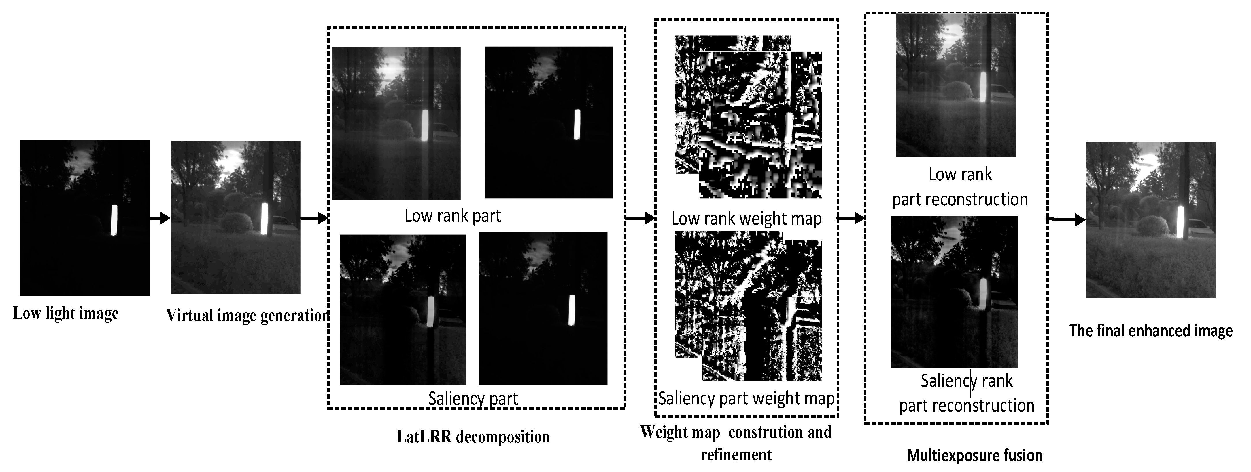
Our framework mainly consists of four main components: (1) Virtual image construction. The optimal virtual image is generated from the original low light image based on the inverse mapping function. (2) Image decomposition and noise suppression. LatLRR is used to decompose the source and the virtual images to obtain the low rank and saliency structures separately. In this process, noise is removed from the image simultaneously. The low rank and saliency parts are processed separately during the subsequent processing. (3) Weight generation, which determines the weight maps of the low rank and saliency parts separately. Additionallyn adaptive optimization model of low-rank weight map is proposed to retain image details and avoid halo artifacts. The total variational method is applied to the establishment and solution of weight maps. (4) Multi-exposure fusion. Two decomposed low rank parts are reconstructed into a new low rank image. In the meantime, two decomposed saliency parts are reconstructed into a new saliency image. Lastly, the two newly images are fused to obtain the final enhanced image. The flowchart is shown in
Figure 1. The detail of each component is described in the following sections.
2.1. Virtual Image Construction
In this step, the linear expansion method based on the global model proposed by Akyüz was used. Specifically, low-light mapping and tone-mapping operators were used on an HDR image to facilitate screen display [
27]. The mathematical model is as follows:
In the original equation, represents the brightness value of pixel in the low-dynamic-range image, represents the brightness value of the HDR image, represents the minimum brightness value that is mapped to white light, and is the initial brightness value based on ratio of the HDR image. Additionally, is a quantification parameter. The larger the value is, the brighter the image after quantization is. is the harmonic mean of the brightness of the HDR image.
In this study, the above equation was introduced to the virtual image construction process, and
was calculated as follows:
Substituting Equation (2) in Equation (1):
Equation (3) is a quadratic equation of
, so
can be obtained by solving the quadratic equation. Since the brightness value of the HDR image obtained by inverse tone mapping cannot be negative, a positive value is set in this study:
For simplification, the variable
is introduced:
. Since the maximum brightness
of the image after inverse tone mapping must be the maximum brightness
in the low-light image, the following equation is obtained:
Assuming that after image normalization, the maximum brightness value of the normalized image is 1, that is,
; then, we have
The virtual image construction operator is obtained:
where
and
=1. In Equations (1)–(7), original images are normalized to [0~1]. So, the intermediate image
is a normalized image. To construct an image with a different exposure ratio from
, the main parameter is
. If
is too high, the low brightness values of the original image will be mapped to very low values in the image
, and the high brightness values in the original image will be mapped close to the maximum brightness value.
Because a well-exposed image can provide rich information for the human eye, to obtain the optimal exposure image, the image information entropy was adopted to automatically calculate the value of
in real time according to the input image. The one-dimensional image entropy is a statistical form of the feature that reflects the amount of average information in an image. The one-dimensional information entropy is calculated as follows:
where
is an image and
represents the image information entropy;
i represents grayscale value in the image
,
;
N1 is the maximum grayscale value of the image,
N1 = 255;
is the probability of grayscale value
I;
is the number of times that the grayscale value
i appears in the image
;
M is the number of image rows; and
N is the number of image columns.
As the value of
increases, the image information entropy first increases and then decreases. Thus, the information entropy can be used to determine the optimal
:
When solving for the optimal
,
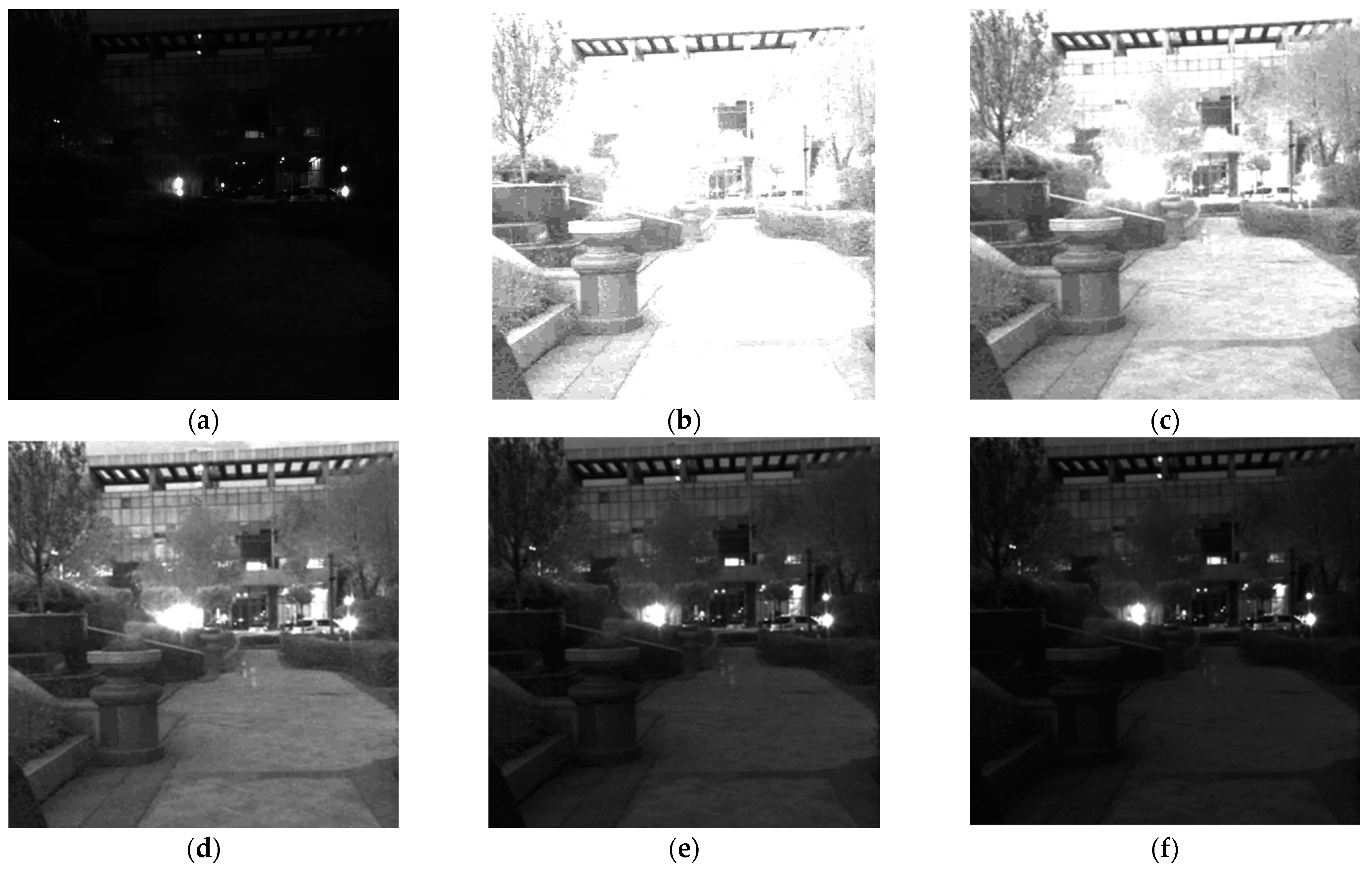
should be mapped to [0~255] to calculate the information entropy. Additionally, the image is down-sampled to reduce the amount of computation. In
Figure 2, image (a) is an original low-light image. Based on Equation (10),
is changed from 20 to 60 (the corresponding normalized value is 20/255~60/255), and the corresponding intermediate image is calculated, as shown in
Figure 2b–f. It can be seen that the information entropies are 3.79, 4.17, 4.85, 4.08, and 3.82, respectively. Obviously, image (d) has the highest information entropy, so it is selected as the optimal image. In the following section, the source image is denoted as
, and
is used as input for
in Equation (7), and the virtual images generated by Equation (7) are denoted as
.
2.2. Image Decomposition and Noise Suppression
Low-light images typically have many noises. To improve the signal-to-noise ratio (SNR) of the enhanced image, LatLRR [
28,
29] was utilized to decompose the source image
and the intermediate image
. LatLRR is efficient and robust to noise and outliers. LatRR decomposes the image into a global structure, a local structure, and sparse noise. The solution model of LatLRR decomposition can be defined as follows:
where
is the equilibrium factor,
denotes the nuclear norm,
is
,
is an image with the size of
,
Z is the low-rank coefficient,
L is the saliency coefficient, and
E is the sparse noise. Then, the low-rank component XZ (
), saliency component LX (
), and sparse noisy component E can be derived. The noise is removed, and only the low-rank and saliency components are input for fusion processing.
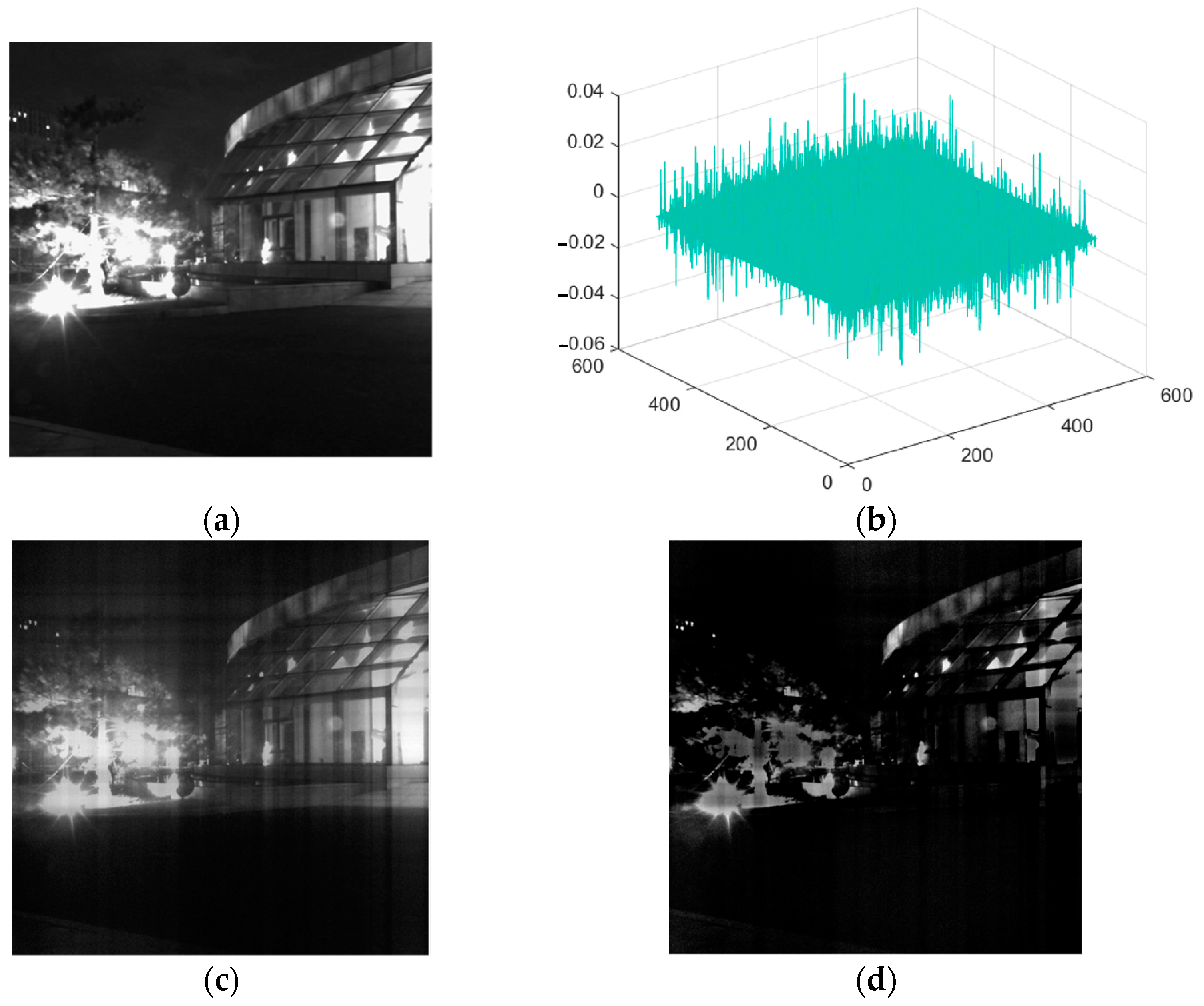
An example of LatLRR decomposition using Equation (11) is shown in
Figure 3. The image in
Figure 3a is the source image.
Figure 3b depicts the noise in the 3D display, which is suppressed using Equation (10).
Figure 3c shows the low-rank component of the image.
Figure 3d depicts the saliency features.
The Equation (11) was utilized to decompose the source image and the virtual image . After low-rank decomposition, the source image was decomposed into and . Additionally, the virtual image was decomposed into and . In this paper, was used to represent the low-rank images, ={,}, and was used to represent the saliency images, ={,}. In the following process, they are treated separately and then fused in the end to remove the noise.
2.3. Weight Generation
For the image enhancement algorithm based on multi-exposure fusion, the weights of the images directly affect the fusion result. In this study, different weight map construction methods were used after decomposition to achieve the best visual effect, avoid the halo artifacts, and preserve as many image details as possible.
2.3.1. Low-Rank Component
The low-rank component contains global information, energy information, and brightness and contrast information about the image. First, a contrast factor is constructed. The initial contrast weight is constructed by Equation (12):
where
is the low-rank image,
is the Laplacian operator,
is the convolutional symbol, and
means the absolute value.
represents a two-dimensional Gaussian filter; the Gaussian filter kernel is 0.5, and the size of Gaussian core is 7.
is the initial contrast weight.
To avoid the halo artifacts and retain details and texture information, a weight map optimization operator
is proposed. The solution equation of
is
where
represents the pixels in the image;
and
are the
norm and
norm, respectively;
and
are weight factors;
and
are the first-order gradient in the vertical and horizontal directions, respectively, in a
neighborhood with
x as the center; and
y represents the pixels within
. In this study,
. The first term in Equation (14) is used to minimize the difference from the initial weight factor, the second term ensures the continuity of the weight factor, and the third is used to preserve the image detail and to avoid the halo artifacts. For convenience, pixel
x is omitted in the expression below.
To solve Equation (14), two intermediate variables are introduced:
and
, and
and
are the first-order gradient of
in the vertical and horizontal directions. Then, the unconstrained Equation (14) is rewritten as
The equivalent of Equation (15) is
where
and
are positive constants. Equation (17) can be solved by a two-step iterative method. The first step is to calculate
and
:
The second step is to calculate
by substituting
and
into the following equation:
According to reference [
30], the L1-norm optimization problem in Equation (18) can be directly solved:
To solve Equation (19), two intermediate variables are introduced, namely,
and
; then, Equation (19) can be decomposed into a forward-splitting component Equation (22) and a backward-splitting component Equation (23) using the proximal forward–backward splitting framework [
30]:
where
is the derivative of
and
t is the iteration step coefficient. Equation (22) can be solved by the relative total variation model as described in [
31].
Up to this point, the decomposition and optimization of the nonlinear problem have been converted into a variational model, and the numerical value of the corrected weighting factor can then be solved through iterations, as shown in Algorithm 1.
| Algorithm 1. Solution Process of the Weight Factor |
| 1: Initialize |
| 2: For k = 0 to K, k is the number of iterations |
| 3: Update and according to Equations (20)–(21) |
| 4: Update according to Equation (22) |
| 5: Update according to Equation (23) |
| 6: End for |
| 7: Output the optimal weight factor |
2.3.2. Saliency Component
The saliency part contains prominent local features and special brightness distributions. This paper proposes as a texture factor of saliency the part designed as Equation (24).
where
is the saliency image,
represents the pixels in the image, and
is the saliency weight map of
. The first term
is the norm of the image, and
is the average value of saliency image.
is a gain parameter and is set to 3.
2.3.3. Weight Normalization
After low-rank decomposition, the low-rank component
={
,
} and saliency component
={
,
} of the source image
and the intermediate image
were obtained, and the weight maps of four images after decomposition were constructed according to
Section 2.3.1 and
Section 2.3.2. The weights of the low-rank components are
and
, and the weights of the saliency components are
and
.
Finally, the weights of the four images need to be normalized:
To achieve good enhancement performance, the weight map of a Gaussian pyramid was generated based on
,
,
, and
. Laplacian Pyramid fusion was also used to obtain the fusion results [
32].
2.4. Multi-Exposure Fusion
To reduce the computational complexity, we only used the source image and the generated intermediate virtual image for fusion. First, the decomposed low-rank images
= {
,
} were fused to obtain
, and the saliency images
= {
,
} were fused to obtain
.
Last,
and
were fused to obtain the final enhanced image:
The steps of the low light image-enhancement method are listed in Algorithm 2.
| Algorithm 2. Low-light grayscale image-enhancement method proposed in this study |
Input: Low-light grayscale image ;
|
Output: Enhanced image ;
|
| 1. Generation of intermediate virtual image by Equations (1)–(10). |
| 2. LatLRR decomposition of the source and intermediate images by Equation (11). |
| 3. Weight map construction of the low-rank component by Equations (12)–(23). |
| 4. Weight map construction of the saliency component by Equation (24). |
| 5. Weight map normalization by Equations (25)–(28). |
| 6. Image fusion by Equations (29)–(31). |
| 7. Output the enhanced image . |
3. Experimental Results and Analysis
In this section, the parameters of the proposed method were first analyzed, and then the proposed method was compared with eight state-of-the-art algorithms [
6,
8,
9,
12,
16,
18,
24,
31] in the aspects of visual effect and objective evaluation indices. On the basis of image dehazing, reference [
12] proposed a model that can directly use the DCP-based method to deal with the inverted image. In reference [
24], the CRF model was used to construct a virtual image, and then the multi-exposure fusion framework was used to achieve image denoising. Reference [
8] was based on Retinex: the light of each pixel was first estimated individually by finding the maximum value in the red, green, and blue channels. Then, the initial light map was refined by imposing a structure prior on it. Reference [
31] was also based on Retinex. It estimated the latent components and performed low-light image enhancement based on a deep learning framework. Reference [
6] is proposed based on the bilateral gamma adjustment function and combined with the particle swarm optimization (PSO), and the algorithm significantly enhanced the visual effect of the low illumination gray images. Reference [
16] proposed a fast and lightweight deep learning-based algorithm for performing low-light image enhancement using the light channel of hue saturation lightness (HSL). This method used a single channel lightness ‘L’ of HSL color space instead of traditional RGB color channels to reduce time consumption. Reference [
9] enhanced the low-light images through regularized illumination optimization and deep noise suppression. Reference [
18] proposed an enhancement method based on GAN (generative adversarial network).
The models selected for comparison involved a typical Retinex model, a DCP dehazing model, a deep learning model, and a multi-exposure fusion framework as shown in
Table 1.
Experiments were carried out using MATLAB 2020a on a computer with an Intel Core i7 3.40-GHz CPU, 16 GB of RAM, and the Microsoft Windows 10 operating system. The machine learning experiments were implemented in in Python 3.8.0 and Python3.8.0 can be downloaded from the website:
https://www.python.org/downloads/release/python-380/ accessed on 3 May 2022.
3.1. Parameter Settings
Most of the existing datasets have only color images, and the algorithm in this study was designed to enhance low-light grayscale images. Thus, a low-light camera (G400BSI) was used to capture low-light grayscale images in this study. The proposed method consists of two types of parameters: (1) the maximum brightness
and
in the virtual image construction step, where
is the normalized brightness value,
= 1. In the proposed method,
is obtained by calculating the information entropy, and
= 10, i.e., the lower limit, to improve the iteration speed. In LatLRR,
= 0.8. (2) is the low-rank weight construction process, the normalization factors
and
are used to balance the ratio, the penalty factors
and
are used to ensure the stability of the solution, and
t affects the speed of the solution. Increasing
causes more blurriness, though many textures are still retained.
controls the smoothness of the weight factors. In this study, many experiments were carried out on these parameters. The cross-checking test method is used. The parameters
and
vary from 1 to 10, and the interval is 1.
and
vary from 1 to 10, and the interval is 1. Additionally, t varies from 0.01 to 2, and the interval is 0.01. The objective evaluation indexes of 20 groups of data (in
Section 3.3) under each set of parameters are calculated, the optimal combination of parameters is found corresponding to evaluation indexes of each set of parameters, and they are chosen as empirical parameters. The final parameter settings were
,
,
,
, and
.
3.2. Subjective Analysis
The captured images were enhanced by different methods. The results are shown in
Figure 4 and
Figure 5. In
Figure 4a there are four low-light images, (b–j) are the results of bio-inspired multi-exposure fusion (BIMEF), low-light image enhancement (LIME), DCP, RetinexDIP, bilateral gamma adjustment function (BGA), hue saturation lightness (HSL), deep noise suppression (DNS), generative adversarial network (GAN), and the method proposed in this study, respectively. Since the images are too large to be included in this manuscript, partially enlarged views are shown in
Figure 4k, and from top to bottom, the images are the results of BIMEF, LIME, DCP, RetinexDIP, BGA, HSL, DNS, GAN, and the proposed method. It can be seen that the results of LIME, DCP, and RetinexDIP showed obvious halo artifacts and significant noise. Specifically, RetinexDIP and BGA over-enhanced the images. In terms of visual effects, DNS, GAN, and the proposed method showed superior performance.
Figure 4k is a partially enlarged view of the third image. The proposed method not only enhanced the details of the dark regions but also preserved the texture of roads. The proposed method yielded significantly lower noise in the roads than the other methods.
Figure 4l is a partially enlarged view of the fourth image. It can be seen that the proposed method enhanced the texture of the details in the house, without any halo artifacts.
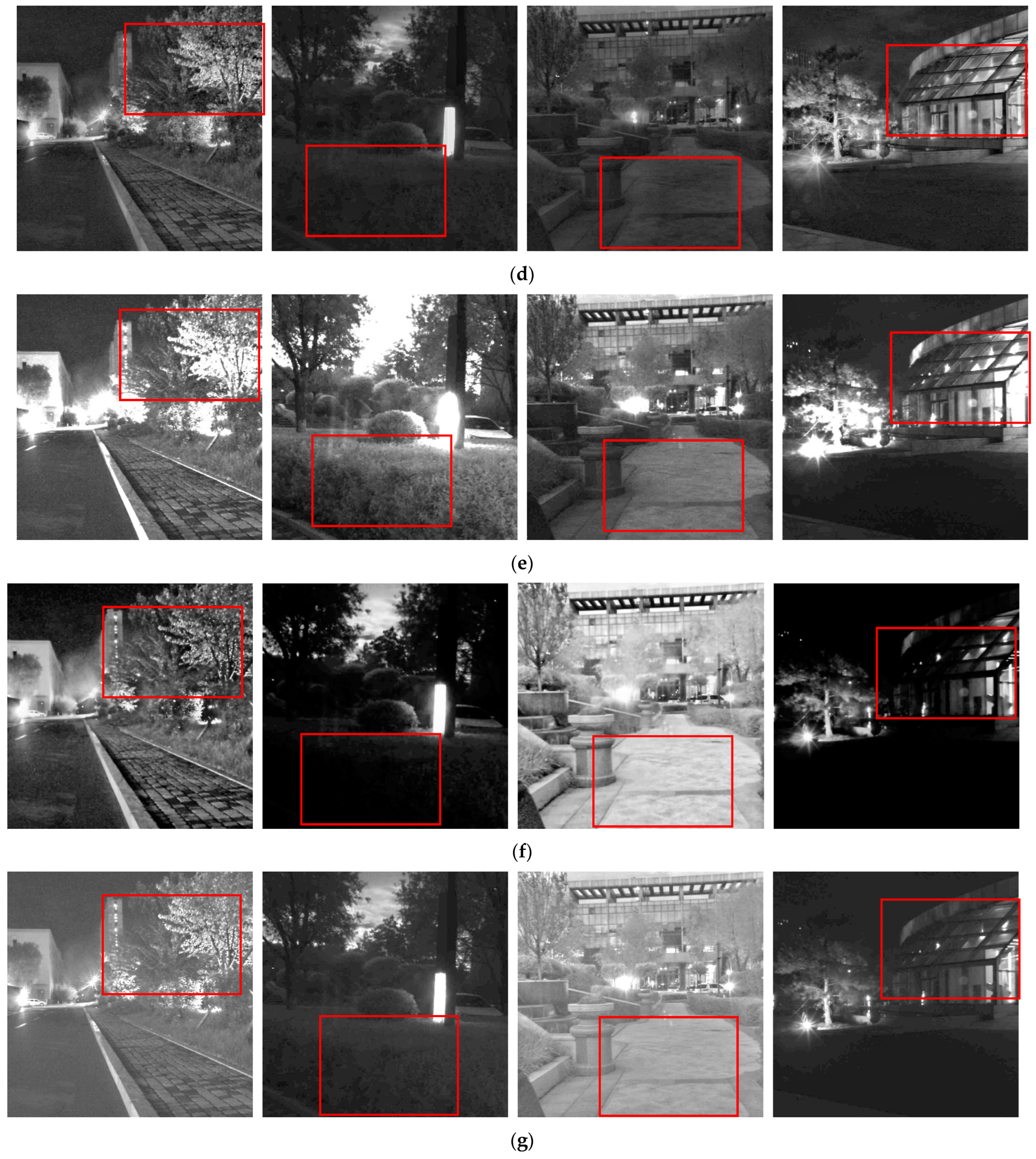
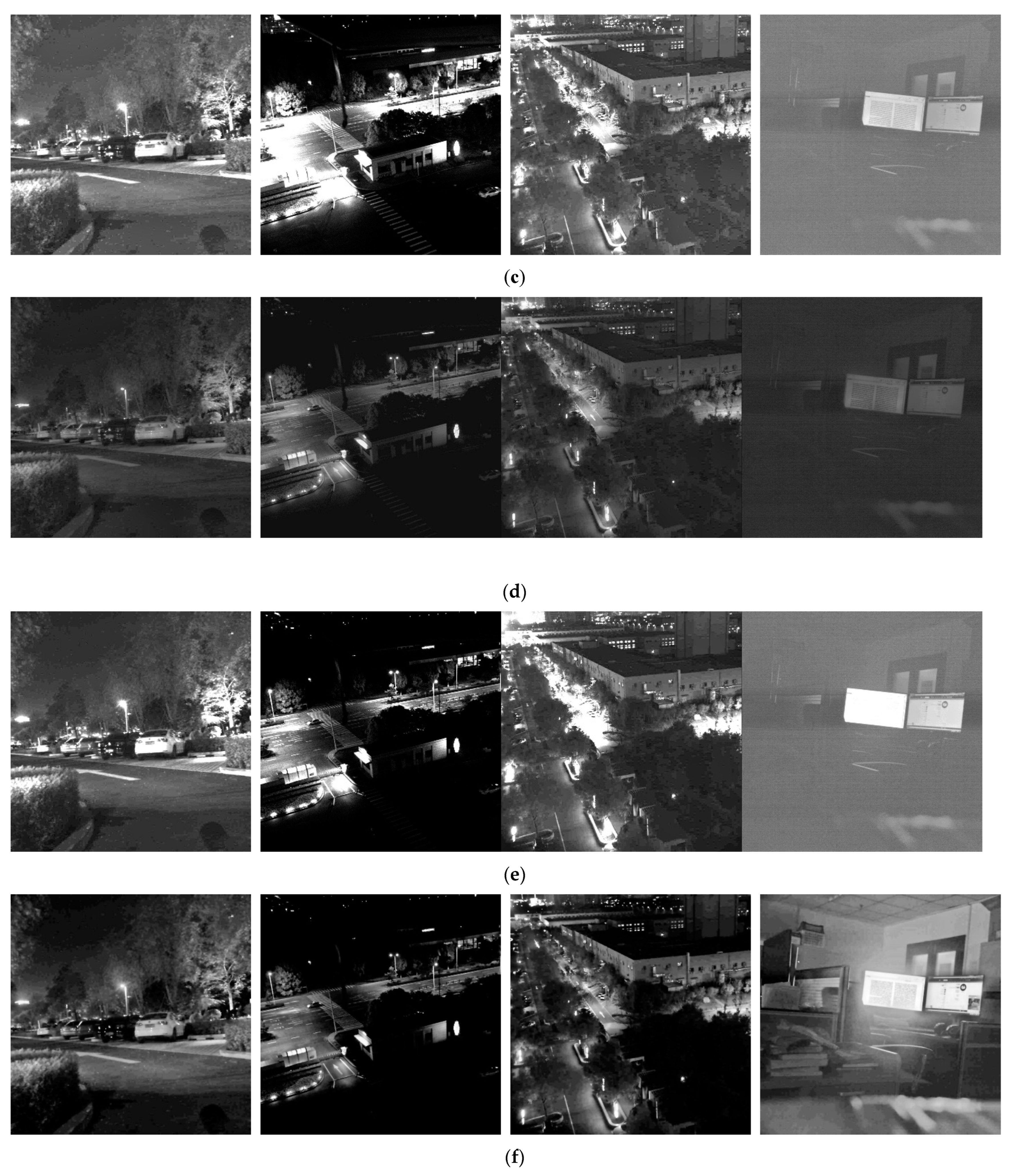
Figure 5a shows four original low-light images.
Figure 5b–j are the results of BIMEF, LIME, DCP, RetinexDIP, BGA, HSL, DNS, GAN, and the method proposed in this study, respectively. It can be seen that LIME and RetinexDIP had obvious halo artifacts. The BGA algorithm results in over- and under-enhancement, as shown in
Figure 5f,; the road of the second image is under-enhanced, and the screen of the fourth is over-enhanced. In contrast, the DNS algorithm works better overall. The GAN method produces halo artifacts on the first image and the third image. The last one of
Figure 5j shows the enhancement result of our method on an indoor image. The proposed method restored the bright screen, as well as the table and book in the dark area. The method proposed in this study retained more detailed information, and the road texture was clear. Additionally, there was no saturation caused by over-enhancement. In
Figure 5k, from top to bottom are the comparison results of 9 methods.
Figure 5k shows the partially enlarged views of the first image. As we can see from the figure, the proposed algorithm does not produce halo artifacts. Moreover, the image noise was significantly reduced.
3.3. Objective Analysis
Three popular full-reference image quality assessment methods—peak-signal-to-noise ratio (PSNR) [
33,
34], structural similarity (SSIM) [
35], and lightness order error (LOE) [
36]—were used to evaluate the enhancement quality by comparing the enhanced image with the ground-truth version. One popular no-reference image quality assessment method—natural image quality evaluator (NIQE) [
37]—was also employed to perform blind image quality evaluation. The larger the PSNR and SSIM and the smaller the LOE and NIQE were, the better the image was, that is, the enhanced image looked more natural.
The PSNR, SSIM, LOE, and NIQE of the five methods are shown in
Table 2,
Table 3,
Table 4 and
Table 5. The index with the best result is written in bold. As seen from the tables, the method proposed in this study did not perform best in every index, but overall it performed better than the other methods. It has obvious advantages in terms of visual effect and denoising indices.
3.4. Time Precision Analysis
The images used in this study were mostly 1000 × 1000 pixels. The average processing time was calculated to compare the performance of the different methods. The number of iterations of LatLRR used in our method was set to 20. RetinexDIP, GAN, HSL and DNS used a GPU for computation. The same parameters as in the original papers are used. Based on the experimental results as show in
Table 6, the BIMEF and LIME methods were relatively fast, whereas the deep learning-based methods were more time-consuming. The method proposed in this study was not the best in terms of computation time, but in terms of the overall performance, it was superior to the other methods.


