Abstract
Agricultural land extent and change information is needed to assess food security, the effectiveness of land use policy, and both environmental and societal impacts. This information is especially valuable in biodiversity hotspots such as the Mediterranean region, where agricultural land expansion can result in detrimental effects such as soil erosion and the loss of native species. There has also been a growing concern that changing agricultural extent in fire-prone regions of the Mediterranean may increase fire risk due to accumulation of fuel in abandoned areas. In this study, we assessed the extent and change of agricultural land in Southern Greece from 1986 to 2020 using a combined European Land Use/Cover Area frame Survey (LUCAS) and Landsat time series approach. The LUCAS data and Landsat spectral-temporal metrics were used to train a random forest classifier, which was used to classify arable land and permanent agriculture (e.g., olive orchards, vineyards) at annual time steps. A post-processing step was taken to reduce spurious landcover class transitions using transition likelihoods and annual class membership likelihoods. A validation dataset consisting of 2666 samples, identified via a stratified random sampling approach and high-resolution imagery and time series analysis, were used to evaluate stable and change strata accuracies. Overall accuracies were greater than 70% and strata-specific accuracies were highly variable between stable and change strata. The results show that southern Greece has experienced a recent gain in arable land (~12,000 ha from ~2009–2020) and a much larger gain in permanent agriculture (>115,000 ha from ~1993–2020). Arable land loss mainly occurred from 1987 to ~2002 when extent decreased by 15,000 ha, of which 66% was abandoned. The semi-automated approach described in this paper provides a promising approach for monitoring agricultural land change and enabling assessments of agriculture policy effectiveness and environmental impacts.
Keywords:
agriculture mapping; arable land; permanent agriculture; Landsat; LUCAS; Google Earth Engine; Greece 1. Introduction
Monitoring expansion and loss of agricultural land extent is critical in wildfire-prone and biodiverse areas such as the Mediterranean region, where changes in agricultural land extent can threaten native species, increase soil erosion, and impact wildfire spread through changes in surface fuel continuity [,,,]. Although Greece is one of the Mediterranean countries that has experienced major socioeconomic and policy changes in the last three to four decades, likely leading to changes in land cover and land use, agricultural extent and change is not well documented. Starting in 1981 when Greece joined the European Union (EU) the country has been subject to regulatory changes due to the implementation of Common Agriculture Policy (CAP), a system with the goals of improving food security and standards of living for farming communities through subsidies and support programs. The economic crisis, starting in 2008, was a significant driver of shifting workforces in rural and urban areas [] resulting in localized evidence of agricultural land abandonment within Greece (e.g., [,]) as well as an increase in agriculture activity in some areas (e.g., [,]). Exponential demand for olive oil since the 1980s, coupled with advances in irrigation technology and increasing EU subsidies for olive oil sector, have likely driven an increase in the extent of permanent agricultural land [,] but few studies have assessed this possibility. In light of these socioeconomic changes, there is an outstanding need for moderate-to-high spatial resolution (e.g., ≤30 m resolution) agricultural land extent products that can serve as baseline data to assess effectiveness of agricultural policies, identify land use change drivers, and understand consequences of agricultural land use change [,].
Satellite observations provide an effective way to map agricultural land at regional to global spatial scales [,,,]. However, mapping agriculture in many areas of the world can be challenging as it is highly dynamic in space and time and can have similar spectral reflectance to natural vegetation. Agricultural practices such as tilling or not tilling, and cover cropping after harvest can have high inter-annual variability in many areas, including Greece [,]. In some cases where CAP regulations are in effect, farmers are paid to keep some of their land fallow or use cover crops to reduce soil erosion []. Tilling practices associated with arable crops and permanent agriculture can occur at similar times of the year, resulting in similar changes in spectral reflectance [,] and map misclassification. Rapid changes in spectral reflectance associated with harvesting and tilling may be missed by lower frequency satellite observations (e.g., Landsat), especially in cloudy times of the year when observations are further reduced []. To minimize these issues, recent mapping approaches have employed time series analyses that take advantage of all available observations. Some of these approaches derive spectral-temporal metrics from Landsat time series data to train machine learning classification algorithms, including decision tree ensembles [] and random forest classifiers [,,], to map agricultural land. Other approaches have utilized observations from other sensors (e.g., Sentinel-2) to fill missing gaps in the Landsat observation record []. Studies have also shown that multi-temporal data can also help differentiate landcover with similar spectral reflectance, such as arable crops and native grasslands in Mediterranean ecosystems [,]. In this study, we extend prior work that utilizes spectral-temporal metrics for mapping landcover through time by including postprocessing steps that have been shown to reduce spurious landcover class transitions in other regions of the world [,,].
Several mapping approaches and products have been used to assess the extent of agricultural areas in Greece and elsewhere in the Mediterranean region. For example, ref. [] used high resolution aerial imagery to map agriculture extent and change in a small area in Central Greece. Other studies have mapped arable land and permanent agriculture extent using Landsat data across all of Europe, but for a single year []. Single year agriculture extent maps are useful but limit longer-term analyses of trends and potential drivers and consequences of landcover and land use change. Agricultural extent data with longer temporal records include landcover mapping products produced through the Coordination of Information on the Environment (CORINE), which provides one of the longest records for landcover change in Europe []. CORINE landcover products have 100 m spatial resolution and were first produced for 1990 and have been produced in approximately six-year intervals since 2000. While the long record of CORINE could be useful for assessing landcover change, previous studies have found that CORINE can have significant overestimation (~63%) of agricultural land []. Additionally, the six-year time span between products is not sufficient for assessing the timing of landcover change, which is important for assessing agricultural land changes such as abandonment [,]. Recent efforts have used Landsat time series data to map agricultural land extent globally from 2000 to 2019 (e.g., []). However, these efforts have concentrated on arable land and have not mapped expansion or loss of permanent agriculture such as olive orchards. The absence of long-term moderate resolution arable and permanent agricultural land products represents a major gap in the current literature and inhibits analyses that seek to understand the drivers and consequences of agricultural land change.
To address this research gap, the main objective of this study was to develop 30 m annual maps of arable land and permanent agriculture extent from 1986 to 2020 in Southern Greece and quantify change over this period. The study focuses on three regions in Southern Greece (Attica, the Peloponnese peninsula, and Crete) that account for a majority of Greece’s permanent agriculture production []. Ground observations derived from the European Union statistical office (EUROSTAT) Land Use/Cover Area frame Survey (LUCAS) and Landsat spectral-temporal metrics were used to train a random forest classifier, which was used to classify arable land and permanent agriculture at annual time steps. A post-processing step was taken to reduce spurious landcover class transitions using a Hidden Markov Model that accounts for landcover class transition likelihoods and annual class membership likelihoods. A validation dataset, derived using a stratified random sampling approach and high-resolution imagery and time series analysis, was used to evaluate map accuracies. The validation dataset was also used to derive a sample-based area estimation for arable land and permanent agriculture.
2. Study Area and Data
2.1. Study Area
The study area covers three regions in southern Greece: Attica, the Peloponnese peninsula, and Crete (Figure 1). Combined, these regions account for ~52% of permanent agriculture production and ~66% of olive tree production in Greece []. With almost 4 million residents [], Attica is the most populated region on the southeast coast of mainland Greece. Annual crops (i.e., cereals) and permanent crops (i.e., olives, grapes) dominate agricultural production (20% and 55% of the total 34 kilohectares (kha) of agricultural land area) []. Intense development, urban sprawl, and real estate speculation in the 1990s and early 2000s, especially near Athens, resulted in greater proportions of fallow agricultural land throughout the region []. The Peloponnese peninsula is located on the southwest coast of mainland Greece. Annual crops (e.g., cereals) and permanent crops (e.g., olives, grapes) dominate agricultural production in Peloponnese peninsula (22% and 69% of the total 543 kha of agricultural land area) []. Crete is the largest Greek island, with mountainous areas that cover nearly half of the island. Permanent crops, and annual crops to a lesser extent, dominate crop production (81% and 9% of the total 277 kha of agricultural land area) []. Small scale studies have identified agricultural land abandonment occurs in the region, especially in marginal growing areas (hilly, mountainous areas) and rural areas, typical of the study area [,,]. Wildfires are common across all three regions in the summer due to hot and dry climatic conditions and fire-prone coniferous forest in the mountains and evergreen shrublands in the lower elevation areas []. These conditions, combined with the country-level major socioeconomic and policy changes, make mapping agricultural change in this area highly relevant and useful for understanding the causes and consequences of this change.
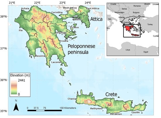
Figure 1.
Study area map showing the distribution of higher elevation mountainous areas and lower elevation valleys and coastal areas. Greece prefecture boundaries are overlaid.
2.2. Data
2.2.1. Landsat Imagery and Preprocessing
We used all Landsat 5 TM, Landsat 7 ETM+, and Landsat 8 OLI Tier 1 surface reflectance imagery from 1986 to 2020 that was available in Google Earth Engine as of May 2021. Required Landsat scenes by path/row included: p183r33, p183r34, p183r35, p184r33, p184r34 for mainland Greece and p182r35, p182r36, and p181r36 for Crete. Landsat 5 and 7 data were atmospherically corrected using LEDAPS [] and Landsat 8 data were atmospherically corrected using LaSRC []. These data were masked to exclude clouds, cloud shadow, and snow/ice using the quality assessment band attributes. Following Yin et al. [], Landsat 8 reflectance was normalized to Landsat 5/7 reflectance using the band-specific linear regression coefficients in Roy et al. [] to minimize reflectance differences between the sensors.
The availability of valid (cloud-free, shadow-free, snow-free) observations had large spatial variation and generally increased toward the end of the time series. Figure 2 illustrates the total annual number of valid Landsat observations for every ~five years throughout the time series. The majority (80%) of the years had at least 15 valid observations for ≥75% of the study area. All of the years had at least 10 valid observations for ≥75% of the study area. Notable exceptions include years such as 2012, when observations were limited for most of the study area as only Landsat 7 data was available.
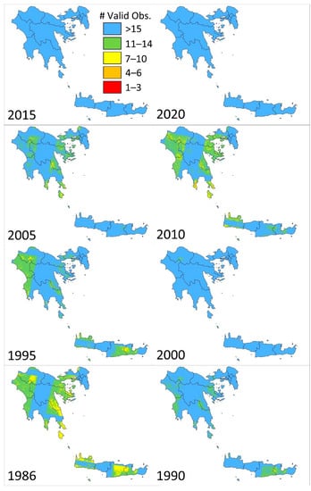
Figure 2.
Total number of annual valid (cloud-free, shadow-free, snow-free) observations across the study area every ~five years throughout the time series.
2.2.2. LUCAS Data
The European Land Use/Cover Area frame Survey (LUCAS) is conducted by the European Union statistical office (EUROSTAT) and provides land cover and land use information across the entire European Union every three years, starting in 2006 []. LUCAS uses a two-phase sampling approach to assess landcover. In the first phase, a systematic grid of points spaced 2 km apart is photo-interpreted and assigned a preliminary land cover class. In the second phase, a stratified sample of points is selected from the first sample and visited in the field by surveyors who assess landcover, land use, and various environmental characteristics. Typically, points located far from roads or those located on private property or other inaccessible areas are either, (1) visually assessed from a distance, or (2) classified as their original photo-interpreted landcover class []. LUCAS data has been used successfully to train landcover classification models that utilize Landsat and Sentinel data [,]. For this study, we acquired all available LUCAS data for the study area in 2009, 2012, 2015, and 2018.
Following the approach used by Pflugmacher et al. [] and Weigand et al. [], we only used LUCAS points that were classified using direct observation at a distance less than 100 m, were assessed for an area greater than 0.5 ha in size and had an assessed landcover proportion of >50%. We did not consider points that classified linear features, such as roads or small waterways. Figure 3 shows the distribution of LUCAS samples across the study area. Table 1 shows the landcover classes used in the following analyses, the associated LUCAS classes, and the total number of LUCAS points used for each landcover class.
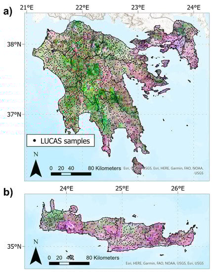
Figure 3.
Distribution of LUCAS samples across: (a) Attica and the Peloponnese peninsula and (b) Crete. Samples are overlaid on Landsat 8 data for the 2020 summer season (June, July, August). Image composite RGB channels represent 90th percentile SWIR1 reflectance, 90th percentile NIR reflectance, and 90th percentile red reflectance, respectively.

Table 1.
Landcover class definitions with corresponding LUCAS classes and number of LUCAS samples used after screening.
3. Methods
3.1. Landcover Classification
Landcover classification was conducted using a random forest classifier. LUCAS samples served as the training dataset. Landsat spectral-temporal metrics and ancillary topographic metrics were calculated for each of the samples using the corresponding year of data and used to train a random forest classifier. This classifier was used to classify landcover across the study area at annual time steps from 1986 to 2020. The following sections describe the training data, predictor metrics, and random forest classification parameters.
3.1.1. Training Dataset
The LUCAS samples served as the primary training dataset for the classification models. The number of LUCAS samples was unbalanced, with some landcover classes having very few LUCAS samples (Table 1). For machine learning classification algorithms, it is common for poorly represented classes in the training dataset to exhibit lower classification accuracy and this issue can be partly remediated by selecting a more balanced training dataset []. Consequently, to create a more-balanced training dataset, we randomly selected 10–20 LUCAS samples of each landcover class in each survey year. Training polygons were drawn on high-resolution Google Earth imagery to include homogenous areas surrounding the target LUCAS point. The resulting training dataset consisted of 14,029 training pixels, with each class having approximately 2000 training pixels.
3.1.2. Classification Predictor Metrics
Classification predictor metrics included spectral-temporal metrics derived using the Landsat data and ancillary topographic metrics. We calculated per-pixel spectral-temporal metrics using six reflectance bands and six spectral indices to use as predictors in our classification models. The six spectral indices used were the Normalized Burn Ratio [], Normalized Difference Vegetation Index [], Bare Soil Index [] and Tasselled Cap Greenness, Wetness, and Brightness [] (Table 2). We calculated both annual and seasonal metrics designed to capture relevant changes in phenology and agricultural practices (e.g., harvest and tilling of annual crops and tilling and grazing the understory of olive orchards to assist harvesting activities and reduce competition for nutrients and fire risk). Seasonal periods included spring (March–May), summer (June–August), and autumn (September–November). Winter was not calculated as there was limited availability of Landsat data during that period, especially early in the time series. For each seasonal period we calculated the median and the standard deviation of the 12 input datasets. Seasonal metrics were calculated for pixels that had three or more valid observations. For the annual time period we calculated the min, max, mean, median, standard deviation, and 10th and 90th percentiles of the 12 input datasets. In addition to spectral-temporal metrics we also included ancillary variables that have been shown to improve classification accuracy in prior studies. We used digital elevation data from the Shuttle Radar Topography Mission V3 product to extract elevation, slope and aspect. We also included geographic latitude and longitude as predictor variables, as [] demonstrated that these variables can improve classification accuracy by capturing spatial relationships of landcover classes. Values for all predictor metrics were derived for each of the training pixel locations using the corresponding year of data (i.e., 2009 training data derived from 2009 Landsat data).
Table 2.
Spectral index formulation and associated reference.
3.1.3. Random Forest Classification
The random forest classifier within Google Earth Engine was used to classify each pixel into one of the seven landcover classes. Random forest is an ensemble learning algorithm that uses bootstrap samples of the training data to train each tree in an ensemble of n trees []. Pixels are assigned the landcover class by majority vote of the ensemble of trees. For this study, the classifier was trained with n = 500 trees and the number of variables at each split was set to the square root of the total number of variables. As our random forest classifier was trained using surface reflectance data, it was considered portable through time [], and we used it to produce annual landcover probability maps from 1986 to 2020. All map outputs were projected in the Moderate Resolution Imaging Spectroradiometer (MODIS) equal-area sinusoidal projection [].
3.2. Time Series Post-Classification Processing
To reduce spurious landcover changes for each pixel through the time series, we applied the post-processing algorithm presented in [] and implemented using the associated Python repository []. The algorithm uses a forward-backward Hidden Markov Model (HMM) to distinguish real and spurious changes in a time series. HMMs use statistical techniques to infer unknown states (i.e., landcover classes) from a sequence of observations (i.e., remotely sensed measurements) in a time series dataset. A forward-backward HMM consists of several components: the initial state probability, or the probability that a particular pixel is a certain landcover class at the initial time, the transition probability, or the probability that a pixel will change between landcover classes from one year to the next, and the state probability, or the probability at each time step that a particular pixel is a certain landcover class, which depends on the transition probability and the previous and following states.
The input to the algorithm consists of the per-pixel initial state probabilities, or the probability that a pixel belongs to each of the n classes in each year of the time series. We used the landcover class membership probabilities generated by the random forest classification for the initial landcover class probabilities for each year in the time series. These images were then combined into one image stack. A forward-backward HMM algorithm was used in conjunction with the transition probabilities, discussed below in this section, to determine the most probable class sequence Ω = {ω1, ω2, … ωn} for each pixel in the stack of yearly class membership probabilities as follows:
where is the probability of observing pixel value xt, given that the true land cover label is ωt. The transition probabilities are derived from the transition probability matrix. This process produced class probabilities for each pixel in each year of the time series. Finally, each pixel was labeled with the most likely class for each year, resulting in annual maps for the entire study area.
The transition probability defines the probability that a pixel will change from one landcover class to another. This transition probability matrix can be estimated from existing landcover maps or other information to estimate the frequency of class-to-class changes, including expert knowledge [,,]. The transition probability matrix is presented in Table 3 and scores the land cover transition probabilities as likely (0.90), probable (0.10), possible (0.025), or not likely (0.001). Stable or no change in landcover class was defined as the most likely outcome, given prior landcover change observations in southern Greece (e.g., []). Examples of probable changes include the succession and densification of natural vegetation from herbaceous to shrubland and shrubland to forest observed in many parts of Greece after disturbance [,,]. Possible changes include transitions from sparsely vegetated to arable land, such as the case of plowed or fallow land being planted with crops the following year. Examples of transitions that are not likely include arable land and herbaceous vegetation to forest, given these transitions would likely take decades in this environment [,].
Table 3.
Land cover transition probability matrix.
As the focus of the study was on landcover change between agriculture and natural vegetation classes we also masked artificial surfaces in the post-processed annual landcover maps using the Joint Research Centre’s Global Human Settlement Dataset [].
3.3. Validation and Area Estimation
A stratified random sampling approach was chosen to assess the accuracy of the resulting maps. The stratification included four stable land cover strata and seven land change strata (Table 4) representing land dynamics for three time periods (1993–1994, 2000–2001, 2016–2017). These time periods were selected to assess whether accuracy changed between periods that used only Landsat 5 data, periods that used Landsat 5 and Landsat 7 data, and periods that used Landsat 7 and Landsat 8 data. These time periods also corresponded to years in the time series when high-resolution Google Earth imagery was available for most the study area. The total sample size for each time period was calculated using the stratified random sampling sample size formula in []:
where N = number of units in region of interest, ) is the standard error of the estimated overall accuracy, Wi is the mapped proportion of area of strata i, and Si is the standard deviation of strata i. We used a standard error for overall accuracy of 0.012. Following the best practices outlined in [], we allocated a sample size of 50 for each change and rare class strata and the remaining samples were allocated proportionally based on the area of each stratum. The target sample size for each time period was 850 and the sampling assessment unit was an individual 30 m spatial resolution Landsat pixel.
Table 4.
Strata and their description, strata weight (Wi) based on the maps of stable and change classes between 1993–1994, 2000–2001, and 2016–2017, and the number of samples per stratum (ni).
The actual land cover strata were derived using visual interpretation of the Landsat time series data (i.e., []) and multi-season Landsat imagery using the Time Series Viewer tool in Google Earth Engine []. Multi-temporal high-resolution Google Earth imagery was also used to aid the strata interpretation. Sample locations were sorted randomly, and the interpreter proceeded to interpret them in order, without knowledge of the mapped strata label. Strata classification accuracy was assessed using confusion matrices calculated between the validation dataset and the landcover map results. Three commonly used classification accuracy metrics (overall accuracy, producer’s accuracy, user’s accuracy) are reported. The sample-based area estimation with 95% confidence intervals was calculated using a stratified estimator following Olofsson et al. [], where the total area for each strata j was calculated as follows:
where Atot is the total mapped area of all strata and is the area proportion for strata j. The standard error of the area proportion was calculated as follows:
where nij is the number of sample pixels in cell i,j of the confusion matrix and Wi is the mapped proportion of area of strata i. Standard error of the estimated area was then calculated as follows:
where is the standard error of the area proportion. The 95% confidence interval was obtained by multiplying the standard error of the estimated area by 1.96, the z-score associated with a 95% confidence interval.
4. Results
4.1. Random Forest Classification and Post-Classification Processing
The number of per-pixel landcover changes between 1986 and 2020 before (A) and after (B) HMM post-processing is shown in Figure 4. The initial annual land cover classification resulted in pixels changing an average of eight (standard deviation: six) times over the time period. A total of 13.6% of pixels experienced no land cover changes, whereas 63.4% changed five or more times. The HMM post-processing substantially reduced the number of changes per-pixel, with pixels changing an average of 0.4 (standard deviation: 0.7) times over the study period. A total of 71.5% of pixels experienced no land cover changes, and only 0.09% changed five or more times.
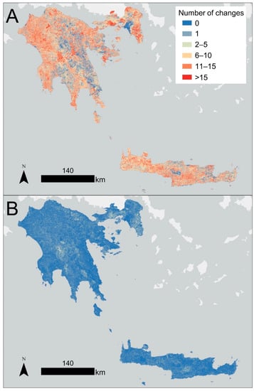
Figure 4.
Number of landcover changes (i.e., the number of transitions from one landcover class to another) from 1986 to 2020 before (A) and after (B) time series HMM post-processing.
4.2. Annual Agriculture Maps and Spatiotemporal Dynamics
We produced study area-wide arable and permanent agriculture maps for the 1986–2020 period along with biennial maps of stable agriculture strata and their conversions. The map of arable and permanent agriculture in the year 2020 is shown in Figure 5. Spatial patterns of arable and permanent agriculture follow expected patterns, where agriculture is generally located in flat coastal areas, valleys and less mountainous areas of the study area. Figure 6 shows two representative sites in the southern Peloponnese and Crete. Both locations illustrate the large variability in agricultural field size, shape, and spatial orientation for both arable and permanent agriculture.
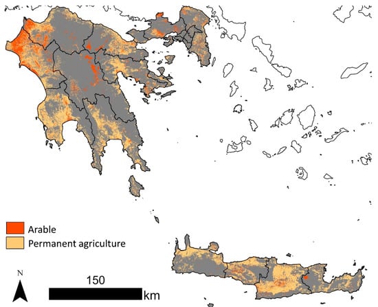
Figure 5.
Arable and permanent agriculture classification map over the study area in the year 2020.
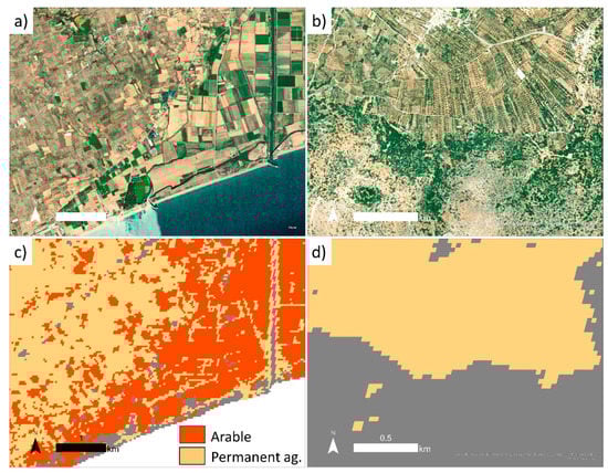
Figure 6.
Arable and permanent agriculture classification examples in the year 2020 for two sites in the study area. Panels (a,c) show true color Maxar imagery and the agriculture classification for an area in the southern Messinia prefecture of the Peloponnese where arable and permanent agriculture are intermixed (centered on 21.997°E, 37.029°N). Panels (b,d) show true color Maxar imagery and the agriculture classification for an area in the Lasithi prefecture of Crete where permanent agriculture is intermixed in evergreen shrubland (centered on 25.663°E, 35.183°N).
Figure 7 shows arable and permanent agriculture extent and change from 1986 to 2020. The map shows proportion of stable and change strata within 10 × 10 km grid cells. Generally, areas that exhibited the largest gain in arable land were in central Crete (Rethymno and Heraklion prefectures). Arable land loss during this time period was mainly concentrated in the central Arcadia prefecture in the Peloponnese. Permanent agriculture exhibited gains in nearly all regions except the central Peloponnese. Permanent agriculture gain was greatest in the west and south regions of the Peloponnese (Messinia and Laconia prefectures) and central Crete (Rethymno and Heraklion prefectures). Areas where arable to permanent agriculture conversion occurred were rare except for a hotspot in the Ilia region of western Greece (Figure 7, bottom left pane). Figure 8 shows example hotspots of arable and permanent agriculture expansion.
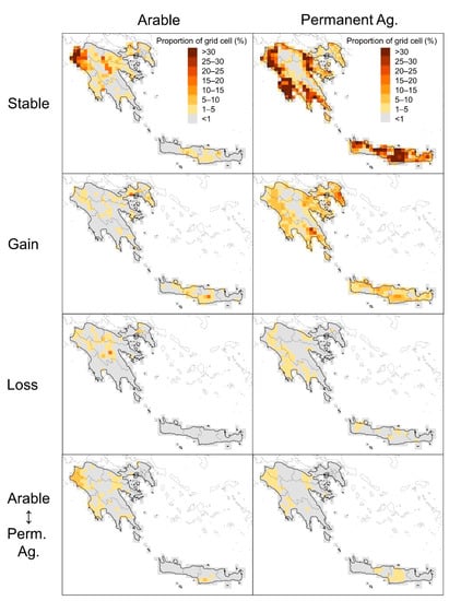
Figure 7.
Arable land and permanent agriculture stable and change strata extent from 1986 to 2020. The map shows proportion of stable and change classes within 10 × 10 km grid cells. For data visualization purposes, we applied a three-year majority filter to the beginning and ending years to reduce the effects of annual crop rotation.
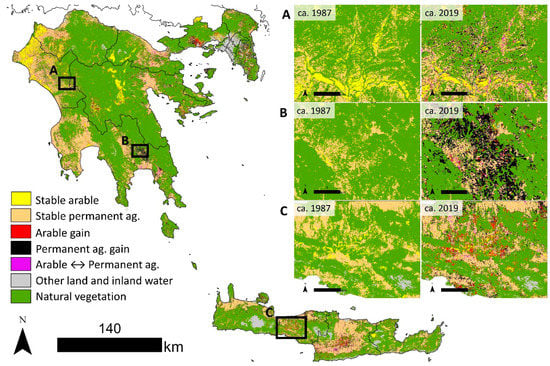
Figure 8.
Selected regional hotspots of arable land and permanent agriculture expansion from circa (ca.) 1987 to 2019. Hotspots of permanent agriculture gain were observed in the Ilia region near Kallithea (A) and in the Laconia region near Geraki (B). Hotspots of arable gain were observed in central Crete, including the Rethymno (C) and Heraklion regions. For data visualization purposes, we applied a three-year majority filter to the beginning and ending years to reduce the effects of annual crop rotation.
4.3. Accuracy Assessment and Sample-Based Area
Stable and change landcover strata for three time periods (1993–1994, 2000–2001, 2016–2017) were evaluated using independent validation data. The overall accuracy of the 1993–1994, 2000–2001, and 2016–2017 maps were 77.3%, 73.6%, and 70.0%, respectively. Strata-specific accuracies were highly variable (Table 5). In general, stable strata had higher producer and user accuracy compared to change strata. Many of the stable strata had higher producer and user accuracies later in the time series (e.g., 2016–2017), likely due to the higher number of annual Landsat observations available compared to early in the time series (Figure 2). Several change strata (arable to permanent ag., permanent ag. to arable, and loss of permanent ag.) had high commission error (>50%) (i.e., classes were identified as change when they were stable) for all three of the assessed time periods. Confusion matrices for the three time periods are presented in Supplemental Tables S1–S3.
Table 5.
Producer’s and user’s accuracies for stable and change strata for the three time periods assessed.
Figure 9 presents mapped extents and sample-based area estimates with 95% confidence intervals for stable and change agriculture strata for three time periods (1993–1994, 2000–2001, 2016–2017). Arable land and permanent agriculture displayed differing temporal trends from 1986 to 2020. Arable land steadily decreased from 1986 to ~2000, with the sample-based area assessment showing a decrease from 179.9 ± 23.8 kha in 1993 to 171.6 ± 24.4 kha in 2000. Starting in ~2009–2010, arable land area increased rapidly to the end of the time series, with the sample-based assessment showing an increase from 171.6 ± 24.4 kha in 2000 to 183.3 ± 31.4 kha in 2016. Permanent agriculture displayed a near-linear increase in area from the early 1990s to the end of the time series. Permanent agriculture area increased from 569.4 ± 56.4 kha in 1993 to 686.5 ± 70.1 kha in 2016.
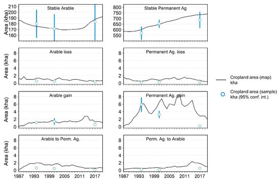
Figure 9.
Map-based and sample-based area estimates for stable and change cropland classes (arable and permanent agriculture). Sample-based analysis was conducted for three time periods (1993–1994, 2000–2001, 2016–2017). Error bars for the area estimates represent 95% confidence intervals. The years on the x-axis represent the last year in each bi-annual period.
5. Discussion
This study sought to map arable land and permanent agriculture extent and change in southern Greece over 35 years using a random forest classifier trained with spectral-temporal metrics and postprocessed to reduce spurious landcover class transitions. The relatively high classification accuracies achieved in this study indicate that the resulting maps could serve as important baseline dataset for analyses that seek to identify drivers and consequences of agricultural land change [,,]. As this study utilized freely available datasets (Landsat, LUCAS) and processing tools (Google Earth Engine, HMM postprocessing), this methodology could be adapted to assess other areas in the Mediterranean and Europe where LUCAS data (or equivalent ground observations) are present to further understand where and when agricultural land is changing. Furthermore, the methodology could be adapted to incorporate other satellite sensor data with similar spectral and spatial characteristics to Landsat (e.g., Sentinel-2) which would provide greater opportunities of suitable observations [] and likely improve agriculture extent and change mapping accuracy.
5.1. Agricultural Extent Dynamics through Time
The mapping analysis performed in this study highlighted two differing temporal trends for arable and permanent agriculture over the 1986–2020 time period. Arable land decreased in area from 1986 to ~2002 and then increased from ~2009 to 2020. While an analysis identifying socioeconomic drivers of agricultural change is beyond the scope of this study, it is notable that peaks in the arable land loss during the 1986–2002 period (Figure 9) are typically within a few years of major CAP changes. For example, peaks of arable land loss around 1989, 1994 and 2002 occur within a few years of production cut agreements and cereal crop subsidy reductions (i.e., 1988 production cut agreement, 1993 MacSharry and Agenda 2000 reforms) []. On average, 66% of annual arable land loss remained non-arable for five or more years, indicating abandonment []. Around 38% of the abandoned arable land was re-cultivated or converted to permanent agriculture by 2020. The arable land increase starting in 2009 is consistent with evidence of people, especially people under the age of 40, returning back to the land when job losses in urban areas (−16%) outpaced job losses in rural areas (−7%) during the first few years of the Greek economic crisis ~2008–2010 []. It is estimated that there was a 15% increase in young farmers alone in the years after the crisis [].
Unlike arable land, permanent agriculture displayed a near-linear increase in extent from the early 1990s to 2020, increasing by >115 kha. Olive oil promotional campaigns and resulting demand, improved olive growing technology, and CAP subsidies are likely drivers of this increase. Marketing and European Union promotional campaigns touting the ‘healthy Mediterranean diet’, with olive oil as a healthy fat, began in the 1980s and likely spurred demand of olive oil [,]. Orchard irrigation technology advances in the early 1990s allowed olive trees to grow in places where they normally could not, which helped increase production of olive oil []. Also, during this time CAP subsidies for the olive oil sector increased from 760 million Euro in the 1980s to over 2300 million Euro in the early 2000s []. Olive producers in Greece have seen direct income transfers via CAP increase from 23% of farm income in 1995 to 28% in 2004 [].
Quantification of agricultural change over time is foundational to understanding impacts resulting from these changes. Mapped changes in agricultural land serve as critical information for evaluating wildfire risk, especially in fire prone areas such as Greece. For example, it has been suggested that abandoned agricultural land can increase fuel continuity and consequently increase fire spread [,,]. There is also evidence that agricultural areas that are typically grazed or tilled annually (e.g., olive orchards) decrease wildfire activity by decreasing surface fuel continuity [,,]. Clearly, there is a need to evaluate how these concurring landcover changes affect fire risk. In addition to fire risk, these maps may serve as an independent source of information for assessing CAP effects and downstream landcover and land use impacts (e.g., soil erosion in tilled olive orchards), which has been a growing concern in the last few decades [,].
5.2. Random Forest Classification and Post-Classification Processing
The HMM postprocessing significantly reduced the number of per-pixel changes between 1986 and 2020. High numbers of pixel changes in time series data before post-processing are not uncommon using random forest classifiers trained with spectral reflectance data [,,]. Typically, these high numbers of pixel changes are caused by missing data, residual noise in the input time series, and poor spectral separability between classes [,]. For example, in Mediterranean environments arable crops can have low spectral separability with natural grasslands and shrublands [,] and could result in a pixel classification changing frequently from year to year. Other classification confusion and inter-annual pixel changes may occur in areas where arable crops (mainly cereals) are planted in the understory of olive orchards, which is prevalent in some areas in Greece []. The results of this study and others (e.g., [,,]) indicate that HMM postprocessing is a valuable tool for stabilizing landcover time series analyses and producing more accurate landcover change products.
5.3. Classification Accuracy and Class Confusion
Stable and change strata accuracies varied widely, with stable strata having higher accuracies in general. Most of the confusion between stable and change strata occurred in the agricultural strata and was likely owing to a few factors. Firstly, agricultural practices such as tilling, not tilling, and/or cover cropping after harvest are not consistent across the study area. In some cases, farmers are paid to keep some of their land fallow or use cover crops to reduce soil erosion []. Tilling results in large changes in spectral reflectance [,] and could affect if a pixel is classified as active agriculture or fallow. Likewise, some farmers also till or graze the understory of olive orchards to assist harvest operations and reduce weeds and reduce fire risk [,]. Tilling and grazing of olive orchards can occur at similar times of the year as arable land harvest and lead to similar changes in spectral reflectance. In the process of map validation, the authors noted that tilling in olive orchards is not a practice that is used everywhere or at a consistent frequency. Secondly, farming techniques such as intercropping could easily lead to strata confusion. Planting arable crops (mainly cereals) in the understory of olive orchards is prevalent in some areas in Greece [] and could lead to confusion when labeling the pixel as arable land or permanent agriculture. Thirdly, geolocation and interpreter errors associated with the LUCAS samples could result in misclassification. Some studies have noted that LUCAS plots can be misinterpreted due to the time of year that they are visited (e.g., pre-crop harvest vs. post-crop harvest []).
5.4. Limitations and Future Work
A limitation of the approach in this paper is that the mapping relied exclusively on Landsat 5, 7, and 8 data, which in some years resulted in reduced observations in certain areas within the study area. The majority (80%) of the years had at least 15 clear observations for ≥75% of the study area and all of the years had at least 10 clear observations for ≥75% of the study area. Notable exceptions include years such as 2012, when observations were limited for most of the study area as only Landsat 7 data was available. Clearly, if a pixel had many observations but was missing observations at key time periods of the year (i.e., harvest of arable crops, tilling olive orchards in late spring), the potential for misclassification would be higher. To overcome the limitation of fewer observations in a season or year, future work will undoubtedly benefit from multi-source and integrated data such as harmonized Landsat-Sentinel-2 datasets [].
While Landsat spatial resolution is sufficient to map agricultural fields in many areas of the world (e.g., [,,]), future work mapping agriculture in areas with small field sizes will benefit from using data with higher spatial resolution. In Greece, nearly 98% of holdings are smaller than 20 hectares [,], and fields can be equal to- or smaller than the width of a Landsat pixel in some areas (e.g., Attica). Within the last 5–7 years, multiple satellite systems with high spatial resolution and high temporal frequency have been operationalized, including the Sentinel-2 satellites and cubesats (i.e., Planet). Studies have achieved high landcover classification accuracy (93%) using 10 m Sentinel-2 imagery []. Likewise, 3 m Planet cubesat data have also been used to map and characterize very small farms (i.e., <600 m2) [].
This study did not use quantitative predictor metric selection methods, such as removing highly correlated metrics, which has been shown to increase the accuracy of random forest classifications [,]. However, other studies have observed that using all possible input variables can result in the highest classification accuracy in certain instances []. Clearly, more work is needed to understand the effects of predictor metric selection on resulting classification accuracies.
6. Conclusions
This study demonstrated the potential of using Landsat spectral-temporal metrics, European land cover survey (LUCAS) and a machine learning classifier for mapping arable land and permanent agriculture extent and change in southern Greece from 1986 to 2020. This mapping approach also showed the utility of using a Hidden Markov Model for reducing spurious landcover transitions in this environment. A total of 2666 validation samples, identified via a stratified random sampling approach and classified via high resolution imagery and time series analysis, were used to evaluate stable and change strata accuracies. As with prior studies, stable agriculture strata exhibited higher producer’s and user’s accuracies compared with change agriculture strata, likely due to the heterogeneous agricultural practices (e.g., till/no-till, intercropping) and inconsistent Landsat seasonal data availability. This study confirms the differing trends of arable land and permanent agriculture observed elsewhere in Greece, with arable land extent decreasing from 1986 to 2000 and increasing after 2009, and permanent agriculture extent increasing annually after 1993. The resulting 30 m annual maps of arable land and permanent agriculture provide detailed information that could be useful for assessing the effectiveness of agricultural policies, erosion and ecosystem degradation, and fire risk at local to regional scales. The annual arable land and permanent agriculture extent maps are freely available for download through PANGAEA Data Publisher for Earth and Environmental Science repository (will add link once application is processed). Future work will explore analyses that can assess the socioeconomic drivers of- and consequences resulting from agricultural land change.
Supplementary Materials
The following supporting information can be downloaded at: https://www.mdpi.com/article/10.3390/rs14143369/s1, Table S1. Confusion matrix for the 1993–1994 time period. UA = User’s accuracy (%), PA = Producer’s accuracy (%). Table S2. Confusion matrix for the 2000–2001 time period. UA = User’s accuracy (%), PA = Producer’s accuracy (%). Table S3. Confusion matrix for the 2016–2017 time period. UA = User’s accuracy (%), PA = Producer’s accuracy (%).
Author Contributions
Conceptualization, A.M.S., L.B. and I.Z.G.; formal analysis, A.M.S. and I.B.; writing—original draft preparation, A.M.S.; writing—review and editing, I.B., L.B., I.Z.G. and C.K. All authors have read and agreed to the published version of the manuscript.
Funding
This work was partially funded by the National Aeronautics and Space Administration (NASA) under award 80NSSC20K1488.
Data Availability Statement
The annual arable land and permanent agriculture extent maps are freely available for download through PANGAEA Data Publisher for Earth and Environmental Science repository (will add link once application is processed).
Acknowledgments
The authors thank the anonymous reviewers for constructive comments that improved the manuscript.
Conflicts of Interest
The authors declare no conflict of interest.
References
- Gómez, J.A.; Llewellyn, C.; Basch, G.; Sutton, P.B.; Dyson, J.S.; Jones, C.A. The effects of cover crops and conventional tillage on soil and runoff loss in vineyards and olive groves in several Mediterranean countries. Soil Use Manag. 2011, 27, 502–514. [Google Scholar] [CrossRef] [Green Version]
- Myers, N.; Mittermeier, R.A.; Mittermeier, C.G.; Da Fonseca, G.A.; Kent, J. Biodiversity hotspots for conservation priorities. Nature 2000, 403, 853–858. [Google Scholar] [CrossRef] [PubMed]
- Pausas, J.G.; Fernández-Muñoz, S. Fire regime changes in the Western Mediterranean Basin: From fuel-limited to drought-driven fire regime. Clim. Change 2012, 110, 215–226. [Google Scholar] [CrossRef] [Green Version]
- Pausas, J.G.; Millán, M.M. Greening and browning in a climate change hotspot: The Mediterranean Basin. BioScience 2019, 69, 143–151. [Google Scholar] [CrossRef] [Green Version]
- Kasimis, C.; Papadopoulos, A.G. Rural transformations and family farming in contemporary Greece. In Agriculture in Mediterranean Europe: Between Old and New Paradigms; Emerald Group Publishing Limited: Bingley, UK, 2013. [Google Scholar] [CrossRef]
- Xystrakis, F.; Psarras, T.; Koutsias, N. A process-based land use/land cover change assessment on a mountainous area of Greece during 1945–2009: Signs of socio-economic drivers. Sci. Total Environ. 2017, 587, 360–370. [Google Scholar] [CrossRef] [PubMed]
- Zambon, I.; Ferrara, A.; Salvia, R.; Mosconi, E.M.; Fici, L.; Turco, R.; Salvati, L. Rural districts between urbanization and land abandonment: Undermining long-term changes in mediterranean landscapes. Sustainability 2018, 10, 1159. [Google Scholar] [CrossRef] [Green Version]
- Apostolou, N. Why Are So Many Young Greeks Turning to Farming? Aljazeera. Available online: https://www.aljazeera.com/features/2017/5/22/why-are-so-many-young-greeks-turning-to-farming#:~:text=Almost%20half%20of%20all%20new,aged%20between%2025%20and%2034 (accessed on 1 July 2021).
- Neves, B.; Pires, I.M. The mediterranean diet and the increasing demand of the olive oil sector. Region 2018, 5, 101–112. [Google Scholar] [CrossRef]
- Scheidel, A.; Krausmann, F. Diet, trade and land use: A socio-ecological analysis of the transformation of the olive oil system. Land Use Policy 2011, 28, 47–56. [Google Scholar] [CrossRef]
- Moreira, F.; Pe’er, G. Agricultural policy can reduce wildfires. Science 2018, 359, 1001. [Google Scholar] [CrossRef]
- Pe’er, G.; Zinngrebe, Y.; Moreira, F.; Sirami, C.; Schindler, S.; Müller, R.; Bontzorlos, V.; Clough, D.; Bezák, P.; Bonn, A.; et al. A greener path for the EU Common Agricultural Policy. Science 2019, 365, 449–451. [Google Scholar] [CrossRef]
- Ramankutty, N.; Evan, A.T.; Monfreda, C.; Foley, J.A. Farming the planet: 1. Geographic distribution of global agricultural lands in the year 2000. Glob. Biogeochem. Cycles 2008, 22, GB1003. [Google Scholar] [CrossRef]
- Pittman, K.; Hansen, M.C.; Becker-Reshef, I.; Potapov, P.V.; Justice, C.O. Estimating global cropland extent with multi-year MODIS data. Remote Sens. 2010, 2, 1844–1863. [Google Scholar] [CrossRef] [Green Version]
- Phalke, A.R.; Özdoğan, M.; Thenkabail, P.S.; Erickson, T.; Gorelick, N.; Yadav, K.; Congalton, R.G. Mapping croplands of Europe, middle east, russia, and central asia using landsat, random forest, and google earth engine. ISPRS J. Photogram. Remote Sens. 2020, 167, 104–122. [Google Scholar] [CrossRef]
- Potapov, P.; Turubanova, S.; Hansen, M.C.; Tyukavina, A.; Zalles, V.; Khan, A.; Song, X.P.; Pickens, A.; Shen, Q.; Cortez, J. Global maps of cropland extent and change show accelerated cropland expansion in the twenty-first century. Nat. Food 2022, 3, 19–28. [Google Scholar] [CrossRef]
- Kizos, T.; Marin-Guirao, J.I.; Georgiadi, M.E.; Dimoula, S.; Karatsolis, E.; Mpartzas, A.; Mpelali, A.; Papaioannou, S. Survival strategies of farm households and multifunctional farms in Greece. Geogr. J. 2011, 177, 335–346. [Google Scholar] [CrossRef]
- Siachalou, S.; Mallinis, G.; Tsakiri-Strati, M. A hidden Markov models approach for crop classification: Linking crop phenology to time series of multi-sensor remote sensing data. Remote Sens. 2015, 7, 3633–3650. [Google Scholar] [CrossRef] [Green Version]
- Yin, H.; Prishchepov, A.V.; Kuemmerle, T.; Bleyhl, B.; Buchner, J.; Radeloff, V.C. Mapping agricultural land abandonment from spatial and temporal segmentation of Landsat time series. Remote Sens. Environ. 2018, 210, 12–24. [Google Scholar] [CrossRef]
- Zheng, B.; Campbell, J.B.; de Beurs, K.M. Remote sensing of crop residue cover using multi-temporal Landsat imagery. Remote Sens. Environ. 2012, 117, 177–183. [Google Scholar] [CrossRef]
- Kovalskyy, V.; Roy, D.P. The global availability of Landsat 5 TM and Landsat 7 ETM+ land surface observations and implications for global 30 m Landsat data product generation. Remote Sens. Environ. 2013, 130, 280–293. [Google Scholar] [CrossRef] [Green Version]
- Xiong, J.; Thenkabail, P.S.; Tilton, J.C.; Gumma, M.K.; Teluguntla, P.; Oliphant, A.; Congalton, R.G.; Yadav, K.; Gorelick, N. Nominal 30-m cropland extent map of continental Africa by integrating pixel-based and object-based algorithms using Sentinel-2 and Landsat-8 data on Google Earth Engine. Remote Sens. 2017, 9, 1065. [Google Scholar] [CrossRef] [Green Version]
- Abdullah, A.Y.M.; Masrur, A.; Adnan, M.S.G.; Baky, M.A.A.; Hassan, Q.K.; Dewan, A. Spatio-temporal patterns of land use/land cover change in the heterogeneous coastal region of Bangladesh between 1990 and 2017. Remote Sens. 2019, 11, 790. [Google Scholar] [CrossRef] [Green Version]
- Pflugmacher, D.; Rabe, A.; Peters, M.; Hostert, P. Mapping pan-European land cover using Landsat spectral-temporal metrics and the European LUCAS survey. Remote Sens. Environ. 2019, 221, 583–595. [Google Scholar] [CrossRef]
- Senf, C.; Leitão, P.J.; Pflugmacher, D.; van der Linden, S.; Hostert, P. Mapping land cover in complex Mediterranean landscapes using Landsat: Improved classification accuracies from integrating multi-seasonal and synthetic imagery. Remote Sens. Environ. 2015, 156, 527–536. [Google Scholar] [CrossRef]
- Abercrombie, S.P.; Friedl, M.A. Improving the consistency of multitemporal land cover maps using a hidden Markov model. IEEE Trans. Geosci. Remote Sens. 2015, 54, 703–713. [Google Scholar] [CrossRef]
- Sulla-Menashe, D.; Gray, J.M.; Abercrombie, S.P.; Friedl, M.A. Hierarchical mapping of annual global land cover 2001 to present: The MODIS Collection 6 Land Cover product. Remote Sens. Environ. 2019, 222, 183–194. [Google Scholar] [CrossRef]
- Hermosilla, T.; Wulder, M.A.; White, J.C.; Coops, N.C.; Hobart, G.W. Disturbance-informed annual land cover classification maps of Canada’s forested ecosystems for a 29-year landsat time series. Can. J. Remote Sens. 2018, 44, 67–87. [Google Scholar] [CrossRef]
- Büttner, G. CORINE land cover and land cover change products. In Land Use and Land Cover Mapping in Europe; Springer: Dordrecht, The Netherlands, 2014; pp. 55–74. [Google Scholar] [CrossRef]
- Yin, H.; Brandão, A., Jr.; Buchner, J.; Helmers, D.; Iuliano, B.G.; Kimambo, N.E.; Lewińska, K.E.; Razenkova, E.; Rizayeva, A.; Rogova, N.; et al. Monitoring cropland abandonment with Landsat time series. Remote Sens. Environ. 2020, 246, 111873. [Google Scholar] [CrossRef]
- HSA/Hellenic Statistical Authority. 2019. Available online: https://www.statistics.gr/en/home/ (accessed on 7 January 2021).
- Salvati, L.; Sateriano, A.; Bajocco, S. To grow or to sprawl? Evolving land cover relationships in a compact Mediterranean city region. Cities 2013, 30, 113–121. [Google Scholar] [CrossRef]
- Papanastasis, V.P. Land abandonment and old field dynamics in Greece. In Old Fields: Dynamics and Restoration of Abandoned Farmland; Island Press: Washington, DC, USA, 2007; pp. 225–246. [Google Scholar]
- EFFIS. European Forest Fire Information System. 2021. Available online: http://effis.jrc.ec.europa.eu/ (accessed on 10 February 2021).
- Masek, J.G.; Vermote, E.F.; Saleous, N.E.; Wolfe, R.; Hall, F.G.; Huemmrich, K.F.; Gao, F.; Kutler, J.; Lim, T.K. A Landsat surface reflectance dataset for North America, 1990–2000. IEEE Geosci. Remote Sens. Lett. 2006, 3, 68–72. [Google Scholar] [CrossRef]
- Vermote, E.; Justice, C.; Claverie, M.; Franch, B. Preliminary analysis of the performance of the Landsat 8/OLI land surface reflectance product. Remote Sens. Environ. 2016, 185, 46–56. [Google Scholar] [CrossRef]
- Roy, D.P.; Kovalskyy, V.; Zhang, H.K.; Vermote, E.F.; Yan, L.; Kumar, S.S.; Egorov, A. Characterization of Landsat-7 to Landsat-8 reflective wavelength and normalized difference vegetation index continuity. Remote Sens. Environ. 2016, 185, 57–70. [Google Scholar] [CrossRef] [PubMed] [Green Version]
- Martino, L.; Fritz, M. New insight into land cover and land use in Europe. In Eurostat: Statistics in Focus; European Commission, Eurostat: Luxembourg, 2008. [Google Scholar]
- Weigand, M.; Staab, J.; Wurm, M.; Taubenböck, H. Spatial and semantic effects of LUCAS samples on fully automated land use/land cover classification in high-resolution Sentinel-2 data. Int. J. Appl. Earth Obs. Geoinform. 2020, 88, 102065. [Google Scholar] [CrossRef]
- Mellor, A.; Boukir, S.; Haywood, A.; Jones, S. Exploring issues of training data imbalance and mislabelling on random forest performance for large area land cover classification using the ensemble margin. ISPRS J. Photogramm. Remote Sens. 2015, 105, 155–168. [Google Scholar] [CrossRef]
- Key, C.H.; Benson, N.C. Landscape Assessment: Ground Measure of Severity, the Composite Burn Index; and Remote Sensing of Severity, the Normalized Burn Ratio; General Technical Report RMRS-GTR-164-CD; USDA Forest Service, Rocky Mountain Research Station: Ogden, UT, USA, 2006. [Google Scholar]
- Tucker, C.J. Red and photographic infrared linear combinations for monitoring vegetation. Remote Sens. Environ. 1979, 8, 127–150. [Google Scholar] [CrossRef] [Green Version]
- Diek, S.; Fornallaz, F.; Schaepman, M.E.; De Jong, R. Barest pixel composite for agricultural areas using landsat time series. Remote Sens. 2017, 9, 1245. [Google Scholar] [CrossRef] [Green Version]
- Crist, E.P. A TM tasseled cap equivalent transformation for reflectance factor data. Remote Sens. Environ. 1985, 17, 301–306. [Google Scholar] [CrossRef]
- Breiman, L. Random forests. Mach. Learn. 2001, 45, 5–32. [Google Scholar] [CrossRef] [Green Version]
- Gómez, C.; White, J.C.; Wulder, M.A. Optical remotely sensed time series data for land cover classification: A review. ISPRS J. Photogramm. Remote Sens. 2016, 116, 55–72. [Google Scholar] [CrossRef] [Green Version]
- Wolfe, R.E.; Roy, D.P.; Vermote, E. MODIS land data storage, gridding, and compositing methodology: Level 2 grid. IEEE Trans. Geosci. Remote Sens. 1998, 36, 1324–1338. [Google Scholar] [CrossRef] [Green Version]
- Friedl, M.A. Land Cover and Surface Climate, Multi-Temporal Land Cover Maps with a Hidden Markov Model (MTLCHMM). 2019. Available online: https://github.com/BU-LCSC/mtlchmm (accessed on 5 May 2021).
- Liu, D.; Cai, S. A spatial-temporal modeling approach to reconstructing land-cover change trajectories from multi-temporal satellite imagery. Ann. Assoc. Am. Geogr. 2012, 102, 1329–1347. [Google Scholar] [CrossRef]
- Giourga, H.; Margaris, N.S.; Vokou, D. Effects of grazing pressure on succession process and productivity of old fields on Mediterranean islands. Environ. Manag. 1998, 22, 589–596. [Google Scholar] [CrossRef]
- Tzanopoulos, J.; Mitchley, J.; Pantis, J.D. Vegetation dynamics in abandoned crop fields on a Mediterranean island: Development of succession model and estimation of disturbance thresholds. Agri. Ecosys. Environ. 2007, 120, 370–376. [Google Scholar] [CrossRef]
- Pesaresi, M.; Ehrlich, D.; Florczyk, A.; Freire, S.; Julea, A.; Kemper, T.; Soille, P.; Syrris, V. GHS Built-Up Grid, Derived from Landsat, Multitemporal (1975, 1990, 2000, 2014). European Commission, Joint Research Centre (JRC) [Dataset] PID. 2015. Available online: http://data.europa.eu/89h/jrc-ghsl-ghs_built_ldsmt_globe_r2015b (accessed on 1 April 2021).
- Cochran, W.G. Sampling Techniques, 3rd ed.; John Wiley & Sons: New York, NY, USA, 1977. [Google Scholar]
- Olofsson, P.; Foody, G.M.; Herold, M.; Stehman, S.V.; Woodcock, C.E.; Wulder, M.A. Good practices for estimating area and assessing accuracy of land change. Remote Sens. Environ. 2014, 148, 42–57. [Google Scholar] [CrossRef]
- Cohen, W.B.; Yang, Z.G.; Kennedy, R. Detecting trends in forest disturbance and recovery using yearly Landsat time series: 2. TimeSync—Tools for calibration and validation. Remote Sens. Environ. 2010, 114, 2911–2924. [Google Scholar] [CrossRef]
- Olofsson, P.; Foody, G.M.; Stehman, S.V.; Woodcock, C.E. Making better use of accuracy data in land change studies: Estimating accuracy and area and quantifying uncertainty using stratified estimation. Remote Sens. Environ. 2013, 129, 122–131. [Google Scholar] [CrossRef]
- Levers, C.; Schneider, M.; Prishchepov, A.V.; Estel, S.; Kuemmerle, T. Spatial variation in determinants of agricultural land abandonment in Europe. Sci. Total Environ. 2018, 644, 95–111. [Google Scholar] [CrossRef]
- Li, J.; Roy, D.P. A global analysis of sentinel-2A, sentinel-2B and Landsat-8 data revisit intervals and implications for terrestrial monitoring. Remote Sens. 2017, 9, 902. [Google Scholar] [CrossRef] [Green Version]
- Ackrill, R. The Common Agricultural Policy; Sheffield Academic Press: Sheffield, UK, 2000. [Google Scholar]
- Food and Agriculture Organization of the United Nations (FAO). FAOSTAT. Available online: http://www.fao.org/ag/agn/nutrition/Indicatorsfiles/Agriculture.pdf (accessed on 7 January 2021).
- Zhu, X.; Karagiannis, G.; Oude Lansink, A. The impact of direct income transfers of CAP on Greek olive farms’ performance: Using a non-monotonic inefficiency effects model. J. Agri. Econ. 2011, 62, 630–638. [Google Scholar] [CrossRef]
- Moreira, F.; Viedma, O.; Arianoutsou, M.; Curt, T.; Koutsias, N.; Rigolot, E.; Barbati, A.; Corona, P.; Vaz, P.; Xanthopoulos, G.; et al. Landscape–wildfire interactions in southern Europe: Implications for landscape management. J. Environ. Manage. 2011, 92, 2389–2402. [Google Scholar] [CrossRef] [Green Version]
- Nunes, M.C.; Vasconcelos, M.J.; Pereira, J.M.; Dasgupta, N.; Alldredge, R.J.; Rego, F.C. Land cover type and fire in Portugal: Do fires burn land cover selectively? Landsc. Ecol. 2005, 20, 661–673. [Google Scholar] [CrossRef]
- Xanthopoulos, G.; Caballero, D.; Galante, M.; Alexandrian, D.; Rigolot, E.; Marzano, R. Forest fuels management in Europe. In Proceedings of the RMRS-P-41: Fuels Management-How to Measure Success: Conference Proceedings, Portland, OR, USA, 28–30 March 2006; Andrews, P.L., Butler, B.W., Eds.; Rocky Mountain Research Station, US Department of Agriculture, Forest Service: Fort Collins, CO, USA, 2006; Volume 41, pp. 29–46. [Google Scholar]
- Zirogiannis, N. Wildfire Prevention and Mitigation: The Case of Southern Greece. Master’s Thesis, University of Massachusetts, Amherst, MA, USA, 2009. [Google Scholar]
- Pantera, A. Initial Stakeholder Meeting Report: Intercropping of Olive Groves in Greece. Available online: https://www.agforward.eu/intercropping-of-olive-groves-in-greece.html (accessed on 7 July 2021).
- Karydas, C.G.; Gitas, I.Z.; Kuntz, S.; Minakou, C. Use of LUCAS LC point database for validating country-scale land cover maps. Remote Sens. 2015, 7, 5012–5041. [Google Scholar] [CrossRef] [Green Version]
- Claverie, M.; Ju, J.; Masek, J.G.; Dungan, J.L.; Vermote, E.F.; Roger, J.C.; Skakun, S.V.; Justice, C. The Harmonized Landsat and Sentinel-2 surface reflectance data set. Remote Sens. Environ. 2018, 219, 145–161. [Google Scholar] [CrossRef]
- Koutsou, S.; Partalidou, M.; Petrou, M. Present or absent farm heads? A contemporary reading of family farming in Greece. Sociol. Rural. 2011, 51, 404–419. [Google Scholar] [CrossRef]
- Rao, P.; Zhou, W.; Bhattarai, N.; Srivastava, A.K.; Singh, B.; Poonia, S.; Lobell, D.B.; Jain, M. Using Sentinel-1, Sentinel-2, and Planet Imagery to Map Crop Type of Smallholder Farms. Remote Sens. 2021, 13, 1870. [Google Scholar] [CrossRef]
- Millard, K.; Richardson, M. On the importance of training data sample selection in random forest image classification: A case study in peatland ecosystem mapping. Remote Sens. 2015, 7, 8489–8515. [Google Scholar] [CrossRef] [Green Version]
- Li, J.; Tran, M.; Siwabessy, J. Selecting optimal random forest predictive models: A case study on predicting the spatial distribution of seabed hardness. PLoS ONE 2016, 11, e0149089. [Google Scholar] [CrossRef]
- Collins, L.; McCarthy, G.; Mellor, A.; Newell, G.; Smith, L. Training data requirements for fire severity mapping using Landsat imagery and random forest. Remote Sens. Environ. 2020, 245, 111839. [Google Scholar] [CrossRef]
Publisher’s Note: MDPI stays neutral with regard to jurisdictional claims in published maps and institutional affiliations. |
© 2022 by the authors. Licensee MDPI, Basel, Switzerland. This article is an open access article distributed under the terms and conditions of the Creative Commons Attribution (CC BY) license (https://creativecommons.org/licenses/by/4.0/).