Article

Object Localization in Weakly Labeled Remote Sensing Images Based on Deep Convolutional Features

1
Guangzhou Urban Planning & Survey Design Research Institute, Guangzhou 510060, China
2
College of Urban and Environment Sciences, Hubei Normal University, Huangshi 435000, China
3
State Key Laboratory of Information Engineering in Surveying, Mapping and Remote Sensing, Wuhan University, Wuhan 430079, China
*
Author to whom correspondence should be addressed.
Remote Sens. 2022, 14(13), 3230; https://doi.org/10.3390/rs14133230
Submission received: 30 March 2022 / Revised: 20 June 2022 / Accepted: 1 July 2022 / Published: 5 July 2022
(This article belongs to the Topic Big Data and Artificial Intelligence)

Abstract

:
Object recognition, as one of the most fundamental and challenging problems in high-resolution remote sensing image interpretation, has received increasing attention in recent years. However, most conventional object recognition pipelines aim to recognize instances with bounding boxes in a supervised learning strategy, which require intensive and manual labor for instance annotation creation. In this paper, we propose a weakly supervised learning method to alleviate this problem. The core idea of our method is to recognize multiple objects in an image using only image-level semantic labels and indicate the recognized objects with location points instead of box extent. Specifically, a deep convolutional neural network is first trained to perform semantic scene classification, of which the result is employed for the categorical determination of objects in an image. Then, by back-propagating the categorical feature from the fully connected layer to the deep convolutional layer, the categorical and spatial information of an image are combined to obtain an object discriminative localization map, which can effectively indicate the salient regions of objects. Next, a dynamic updating method of local response extremum is proposed to further determine the locations of objects in an image. Finally, extensive experiments are conducted to localize aircraft and oiltanks in remote sensing images based on different convolutional neural networks. Experimental results show that the proposed method outperforms the-state-of-the-art methods, achieving the precision, recall, and F 1 -score at 94.50%, 88.79%, and 91.56% for aircraft localization and 89.12%, 83.04%, and 85.97% for oiltank localization, respectively. We hope that our work could serve as a basic reference for remote sensing object localization via a weakly supervised strategy and provide new opportunities for further research.

1. Introduction

Advances in satellite technology have greatly improved the human ability to observe the Earth surface in recent years [1,2]. With the tremendous progress in sensor technology, the quality and quantity of remote sensing images have also undergone remarkable improvements. Consequently, large-scale remote sensing images with high spatial and spectral resolution, which provide abundant and detailed information of ground objects, can be conveniently accessed. Thus, visual object recognition, which aims to determine the location and category of ground objects, has been intensively approached to interpret the content of remote sensing images and better understand our planet [3,4,5,6,7,8,9].
In the past years, object recognition problem are typically addressed by object detection and localization, which have attracted increasing attention [3,7,10,11,12,13,14,15,16,17,18]. It should be noted that there is a subtle difference between object detection and localization. Specifically, object detection aims to extract the accurate extent of every object from a given image scene, where a detected object is typically indicated with a bounding box, either in horizontal, oriented, or polygon styles [6,10,11,19]. In contrast, object localization requires an object in the given image scene been recognized with its position but usually without extent information [17,19,20]. However, the topic of object localization has been rarely addressed in the remote sensing community. Intuitively, determination of object locations is of paramount importance for a user to grasp the spatial distribution pattern of objects in a remote sensing image. Furthermore, the location information of objects of interest is the essential attributes reflected by remote sensing images and forms the cornerstone of a wide range of practical applications such as vehicle surveillance [21] and military target reconnaissance [22].
In this work, we focus on object localization in remote sensing images. Although remote sensing object localization can be achieved through a fully-supervised object detection pipeline, it suffers from the limitation of large-scale instance-level annotations that are labor-intensive and time-consuming [6,7]. When labeling the instance-level bounding-boxes, the rich and complex object background information contained in remote sensing images may introduce annotation noises inadvertently, and thus, impart difficulty to object detection. Moreover, the variance of object properties such as orientation, scale, and viewpoint in remote sensing images also makes the object localization a much challenging task in aspects such as region proposal, bounding-box regression, and semantic classification [3,23,24]. Faced with this situation, localizing objects with the position information using only image-level annotations, i.e., whether or not objects of interest are contained in a remote sensing image, is of great importance to perform remote sensing object recognition. With the aforementioned motivation, we address object localization in the form of (x, y) positions rather than the bounding boxes using weakly labeled remote sensing images based on deep convolutional neural networks (DCNNs). Generally, we proposed a weakly supervised learning framework that utilizes image-level semantic label to achieve accurate localization of multiple objects in remote sensing images based on convolutional neural networks. In addition, a dynamic local response extremum updating method is developed to determine the location of objects using the object discriminative localization map that combines the fully connected and convolutional layer features to indicate the regions of multiple objects in an image.The main contributions of this paper are as follows.
(1) We propose a weakly supervised learning (WSL) framework based on convolutional neural networks (CNNs) for remote sensing object localization using only image-level labels, where semantic scene classification is conducted for the determination of object category. The semantic and spatial feature integration achieved by backpropagating the fully connected feature to convolutional feature is introduced to generate an object discriminate localization map (ODLM) that indicates the salient regions of objects in an image.
(2) A dynamic updating method of local response extremum is proposed for object localization in remote sensing images based on the object discriminative localization map (ODLM), of which the dynamic threshold based on the extremum value is designed to suppress the noise of object response information. The proposed object localization method adapts well to objects of different types, even when the number and positions of objects vary in an image.
(3) Extensive experiments on the localization of different types of remote sensing objects (i.e., airplane and oiltanks) are carried out. The experimental results show that the proposed object localization method can outperform the state-of-the-art ones, demonstrating the rationality and effectiveness of the proposed framework.
The rest of this paper is organized as follows. Section 2 introduces the relevant studies on weakly supervised object detection and localization. Section 3 presents the proposed framework for object localization using only weakly labeled remote sensing images. Experimental results and analyses are presented in Section 4. Finally, in Section 5, we draw conclusions regarding this work.

2. Related Work

As a challenging problem that arose first in the computer vision community, weakly supervised object detection and localization have played a significant role in developing new image interpretation systems and received dramatic attention in the past years [17]. Since powerful feature representation is of great significance to establish a high-performance object localization system, many researchers have dedicated significant effort to develop feature descriptors to localize various types of objects, such as the histogram of oriented gradients (HOG) [25], scale-invariant feature transform (SIFT) [26], and bag-of-visual-words (BoVW) [27]. Based on the powerful representation ability of HOG, many researchers have explored its functionality in weakly supervised object detection [28,29,30]. To tackle the challenge of object detection in shape variation, the deformable part model (DPM) is employed for weakly supervised object detection based on the improved version of HOG features [29,31,32]. As objects with the same category may vary in appearances such as scale, orientation, and brightness, SIFT feature is intensively explored for weakly supervised object detection owing to its robustness in describing the local key information for discriminating different objects [33,34,35]. Lab color is employed to differentiate the objects for their appearance difference in color space [35,36]. In order to enhance the description ability for objects, the shallow vision feature is usually encoded as higher level representations for weakly supervised object detection, such as BoVW [29,33,36,37] and Fisher vector feature [38]. Han et al. [39] proposed a weakly supervised learning strategy for object detection by jointly exploring saliency, intraclass compactness, and interclass separability to initialize a training example set in a Bayesian framework. Zhou et al. [40] integrated the negative bootstrapping scheme into a WSL framework to achieve effective target detection in remote sensing images. Zhang et al. [41] used weakly supervised learning combined with saliency-based self-adaptive segmentation, a negative mining algorithm and a negative evaluation mechanism for object recognition in remote sensing images. These methods have achieved significant success in weakly supervised object detection and localization with the well-designed low-level features. However, designing a stable and powerful feature for object representation is a difficult problem owing to the complexity and variance of image content. Consequently, the detectors based on low-level features inevitably face challenges in generalization ability.
Recently, weakly supervised object detection and localization based on deep learning method have received unprecedented attention and achieved favorable performance in the past years [19]. The deep learning method represented by convolutional neural networks have witnessed a great success in image classification [42,43,44,45,46,47] and the object detection [3,7,11,13,23,24] domain owing to their adaptive feature learning ability. Inspired by this success, convolutional neural network has been widely employed for candidate object discovery, object feature representation, and semantic category determination that significantly advance the performance of weakly supervised object detection and localization. Readers may go to the review papers [17,19] for a more comprehensive perspective of weakly supervised object detection and localization works. Generally, the current mainstream of weakly supervised object localization and detection based on convolutional neural network can be basically categorized into two groups, i.e., multiple instance learning (MIL) and discriminative region localization methods.
In the MIL pipeline, an image is usually decomposed into a bag of individual region proposals, namely instance proposals, based on which feature extraction and semantic classification are performed for object localization and category determination [48,49,50,51,52,53,54,55,56]. In order to acquire accurate localization result, numerous methods are designed to generate region proposals, including selective search (SS) [57], edge boxes (EB) [58], and sliding window (SW) methods. The SS-based method is employed to generate proposals by exhaustive searching of homogeneous regions in an over-segmented image [51,52,53]. The EB-based methods first generate edge features of objects and then produce proposals using the circumscribed rectangles of relevant edges [48,49,50,56]. The SW-based methods generate multi-scale and multi-aspect ratio proposals at each position in the image or feature maps [53,54,55]. Zhang et al. [59] proposed a coupled CNN-based WSL method that combines a candidate region proposal network and a localization network to extract the proposals and simultaneously locate the aircraft. Benefiting from the prior knowledge of location provided by region proposals, the MIL-based methods are able to detect multiple objects with the same semantic category in an image and have achieved significant success for weakly supervised object detection and localization. However, the performance of object detection and localization using MIL-based methods is vulnerable to the influence of incomplete annotation information in the object bags. Moreover, the MIL-based methods usually fall into a multi-step pipeline which is puzzled by the time-consuming procedure of object proposal generation.
In the discriminative region localization pipeline, deep features are activated with excitation backpropagation to generate visualized heatmaps that spotlight objects of interest [60,61,62,63,64,65,66,67,68]. To obtain the discriminative region of objects, a class activation map (CAM) [60] is produced by a weighted assumption of feature maps using the classification layer and the last convolutional layer. However, the generation of CAM usually requires a convolutional feature layer and classification layer with Softmax to be adjacent at the end of a network. In order to generate class discriminative regions, Grad-CAM [61] is proposed by backpropagating the classification score of an image to the convolutional feature layer. Moreover, the Grad-CAM++ [69], Ablation-CAM [70], and Score-CAM [71] are intensively developed to generate more accurate and smoother class activation maps to better indicate the regions of objects. With the extracted discriminative regions, localization of objects are typically performed by using the segmentation technique. To improve the localization accuracy, WCCN [72] is proposed to use cascaded network that trains object segmentation using the class activation maps. ACoL [63] introduces an adversarial complementary learning strategy for object segmentation using two parallel-classifiers. However, segmentation usually produces a mask that covers the entire object instance, but it cannot distinguish whether the region is an object of interest [73]. To alleviate this issue, the segmentation-detection collaborative strategy is proposed by unifying the MIL and segmentation method [50,51]. Owing to the end-to-end training and inference pipeline, the CAM-based object detection and localization methods have an advantage in efficiency when comparing with the MIL-based ones. Thus, the discriminative region localization pipeline has become one of the most popular strategies for object detection and localization in a weakly supervised learning way.
However, the discriminative region localization pipeline based on CAM focuses on localizing a single instance in an image. There may even exist more than one proposals around an object, the CAM-based methods tend to spotlight the most discriminative part of the object rather than the whole object extent. The reason behind the phenomenon lies in that the networks tend to learn the most compact features for image classification while suppressing less discriminative ones [66,74]. That is, in the discriminative region localization pipeline, the performance of object detection and localization relies heavily on the quality of the class activation map. To alleviate the above problems, we address object localization in remote sensing images by leveraging the proposed object discriminative localization map that combines the deep convolutional and fully connected features. Specifically, we aim to localize multiple objects but without extent in remote sensing image scenes. Inspired by the CAM-based methods [60,61] for single object localization, our framework transits the objects’ semantic information contained in fully connected layer to the convolutional layer so that the regions of multiple objects can be distinctly discriminated for location determination.

3. Methods

In this section, we introduce the main procedures of the proposed remote sensing object localization framework. First, the widely used DCNN frameworks are introduced for remote sensing image scene classification, and then we present the ODLM generation scheme for object localization based on the DCNN frameworks. Finally, a dynamic updating method of local response extremum is proposed for object location extraction based on the visualized object localization map. The overall framework is presented in Figure 1.

3.1. Scene Classification

The task of remote sensing object localization mainly covers two key problems. One is the categorical determination for the objects in an image, and the other is the positional information extraction for each object. In this paper, a DCNN model is trained for image scene classification using the image-level labels. Then, the object’s category is determined by the remote sensing image scene classification result. DCNN frameworks have been widely employed for remote image scene classification because of their elaborate structural designs and robust performance [75,76,77]. The conventional DCNN framework typically consists of several basic modules, such as the input layer, convolutional layer, down sampling layer, fully connected layer and output layer. The input layer is used to receive the original image for data preprocessing. A convolutional layer receives data from its previous layer(s) and computes the convolutional features via a certain number of kernels. To enhance the nonlinearity of a DCNN framework, a convolutional layer is typically followed by an activation layer, such as a rectified linear unit (ReLU) [42], leaky ReLU (LReLU) [78] or an improved parametric ReLU (PReLU) [79], among others. These operations can also significantly expedite the convergence of the training procedure and improve the generalization capacity of the network. The down sampling layer is applied to map the feature maps via an average or max pooling operation, which can compress the spatial dimension of the feature maps and reduce the computational load. Typically, several fully connected layers follow a convolutional layer or a pooling layer and transform the convolutional features into a vector feature. The output layer receives input from one or several fully connected layers and outputs the final predicted classification result. The predicted class of a remote sensing image scene indicates whether one or more objects of interest exist in an image. Thus, the image scene classification result is vital to the object’s categorical determination. In addition, effective object feature representation information can also be acquired via the high-performance DCNN classification model, which provides a valid foundation for the subsequent object location information extraction. The top part of Figure 1 shows the main process of scene classification as introduced above.

3.2. ODLM Extraction

The key to acquire an object’s location information is to extract the object’s discriminative map based on the learned deep features for image classification. In this section, we establish the weakly supervised object localization framework by addressing the convolutional and fully connected features in the CNN framework. Typically, a CNN framework processes the raw image through a certain number of convolutional layers and outputs the image’s feature maps at the last convolutional layer. Specifically, a convolutional layer processes the image using shared convolution kernels, which are able to retain the spatial properties of the image content. The down-sampling (e.g., max pooling [80]) and regularization (e.g., ReLU [42]) operations are able to filter redundant information, and thus, retain the semantic information of specific objects for class recognition. Therefore, the last convolutional layer can be regarded as the image’s spatial feature layer, which contains the object’s localization information. Our goal is to integrate the spatial feature maps from the last convolutional layer and generate the localization map corresponding to the image content inspired by [60,61].
On the other hand, the vector features for image representation are typically extracted from the fully connected layers and involved in the final classifier to predict the semantic category of the image. For those images with the same category, a CNN classification model can be trained to extract features with strong correlation owing to their shared semantics. That is, the vector feature should be class-discriminative and therefore reflect the properties of the image object. Our aim is to extend the class feature to the convolutional layer to produce the spatial feature that contains discriminative regions of categorical objects. Thus, a combination of the spatial feature and object’s class feature can be achieved, which helps to generate the ODLM. Typically, each code in the class feature reflects the importance of discriminating a certain class in the feature space. Therefore, we backpropagate the class feature to the last convolutional layer as weights of the spatial feature maps, which are finally integrated to generate the corresponding ODLM introduced from [62]. Specifically, let M i ( x , y ) denote the activation value of the i-th spatial feature map at position ( x , y ) and a q the activated code at the q-th dimensionality of the vector feature. The contribution of the vector feature learned from M i ( x , y ) can be calculated as follows:
w i ( x , y ) = q Q a q M i ( x , y )
where Q is the length of the extracted vector feature. Based on this operation, the contributions of the spatial feature map at each position ( x , y ) can be easily acquired. However, the final extracted vector feature may not be sufficiently pure for class discrimination since it contains noises from the original image or shows instability because of the model training. Taking this situation into consideration, we regard the contribution of the i-th spatial feature map at every position as a whole and calculate the i-th spatial feature map’s contribution by the following operation:
W i = ( x , y ) w i ( x , y )
Since the last convolutional layer typically contains a certain number of spatial feature maps, the final ODLM can be obtained by the weighted sum of the spatial feature maps:
O D L M = i n W i j n W j M i ( x , y )
where n is the number of spatial feature maps. Based on this method, we can visualize the object localization information contained in the deep spatial and vector features, which also help us to recognize the nature of the deep convolutional and fully connected features.

3.3. Object Localization

By employing the method described above, we can obtain the corresponding ODLM, which is actually the object’s position-sensitive map. Moreover, the ODLM picture can effectively indicate the salient regions of objects. Not content with the above results, we aim to further determine the accurate positions of objects. In addition, a remote sensing image may include more than one object, and different objects may manifest different levels of response values. Therefore, a simple thresholding segmentation method may not be effective to adapt to extract the object centers from an ODLM. Faced with this situation, a dynamic local response extremum updating method is developed to further extract the centers of objects in an image.
Specifically, a mean filter is first used to smooth the abnormal response values in an ODLM by
h ( x , y ) = 1 s z ( x , y ) L ( x , y )
where the L ( x , y ) is the response value in a filter window in an ODLM, and where s and z represent the width and height of a mean filter window, respectively. h ( x , y ) denotes the smoothed pixel values of an ODLM. Due to the effects of noises and the instability of model training, some regions may show slight responses which appear as small values relative to the most salient response values in an ODLM. To overcome this problem, a dynamic threshold based on the extremum value of an ODLM is set to suppress the slight noise response information by
t = ( m a x   h ( x , y ) m i n   h ( x , y ) ) θ + m i n   h ( x , y )   = θ m a x   h ( x , y ) + ( 1 θ ) m i n   h ( x , y )
where θ [ 0 , 1 ) is a parameter set to acquire an appropriate threshold t for generating the noised-suppressed ODLM by
h ( x , y ) =   m i n   h ( x , y ) ,   i f   h ( x , y ) < t   h ( x , y ) , i f   h ( x , y ) t
For the same θ , the threshold of t varies considerably between different ODLMs since the extremums of the object response values are different. Nevertheless, by simply normalizing the smoothed ODLM to [ 0 , 1 ] , Equations (5) and (6) can be effectively optimized as
h ( x , y ) =   0 ,           i f   h ( x , y ) < t   h ( x , y ) , i f   h ( x , y ) t t [ 0 , 1 )
where t is the only threshold for generating the appropriate noised-suppressed ODLM. In this work, multiple thresholds denoted by T = { t 1 , t 2 , , t p } are applied to remove the noise effects.
Through the above operations, a refined object position-sensitive map of the ODLM can be obtained. In fact, the salient areas in an ODLM correspond to object positions. A larger response value corresponds to a higher likelihood that the corresponding position holds an object. Therefore, the local extrema are dynamically updated to further extract object localization as follows:
σ = m a x   H s z ( x , y )
p ( x , y ) =   0 ,       i f   h ( x , y ) < σ   h ( x , y ) , i f   h ( x , y ) σ
where H s z ( x , y ) are the pixel values from the refined object response map of the ODLM in a filter window that shares the same size as the former mean filter. Generally, we perform the above operations in the form of a sliding window with a step length of 1. In this way, the refined response map is processed by extracting a continuous local extremum, which we refer to as the dynamic extremum updating method. After this processing, an image with the object location information can be acquired by the different connected components that indicate the positions of objects. Finally, the accurate location of an object can be determined by calculating the center of each connected component as ( 1 k p x , 1 k p y ) , where ( p x , p y ) are the coordinates and k is the number of the pixels in the connected components. By combining the main procedures of remote sensing scene classification, ODLM extraction, and object localization as a whole, our proposed object localization framework using only image-level labels is established, as shown in Figure 1.

4. Experimental Results

4.1. Experimental Setup

4.1.1. Dataset Description

The proposed framework is evaluated on a large-scale remote sensing image dataset containing 2 classes with target images and 23 classes with scene images collected from MapWorld (MapWorld web site: https://map.tianditu.gov.cn, accessed on 30 June 2022) and Google Map (Google Map web site: https://www.google.com/maps, accessed on 30 June 2022) by referencing the RSD46-WHU dataset [62]. The 2 classes with target images include oiltank and aircraft objects to be localized. The oiltank class has 500 images while the aircraft class has 831 images. For the model training, 400 images from each class are randomly selected as the training dataset and the remaining images as the test dataset. Finally, there is a large-scale object set with 464 aircrafts and 572 oiltanks that need to be localized. However, the proposed localization method is based on a DCNN framework and 2 target classes with only 800 images are insufficient to effectively train a suitable DCNN model, which may lead to overfitting for model training. Therefore, the 23 scene classes (namely, agricultural, airport, basketball court, bridge, building, container, fishpond, footbridge, forest, greenhouse, intersection, overpass, parking lot, playground, residential, river, ship, solar power area, square, tennis court, water, wharf, and workshop) are used as a supplement of the background classes. For the sake of fairness, each of the background classes also consists of 400 images as the training dataset together with the oiltank and aircraft training images. Two samples of each class are shown in Figure 2. The spatial resolution of the scene images ranges from 0.5 m per pixel to 2.5 m per pixel, and the image size is 256 × 256 pixels. Typically, the aircraft and oiltank objects are characterized with various scales, with the size changing from a dozen to hundreds of pixels. Each image may contain one or several objects, and each object may appear at any location in the image. In addition, the illumination changes strongly for different images and the background of each object varies dramatically. Each of these factors poses challenges to the performance of our proposed weakly supervised object localization method.

4.1.2. Implementation

As introduced before, the experiments are performed using the popular AlexNet [42] and VGG-16 [43] frameworks considering their reliable image representation ability by the fully connected layers. The AlexNet network consists of five convolutional layers followed by three fully connected layers, which constitutes a shallow CNN framework. The VGG-16 network is composed of thirteen convolutional layers followed by three fully connected layers, which is known as a deep CNN framework. Generally, we use the described dataset to train the image classification models based on these networks. Then, the proposed method is employed to conduct the weakly supervised object localization. To satisfy the input conditions, all images are resized to 227 × 227 pixels for AlexNet and 224 × 224 pixels for VGG-16, respectively. For the training dataset, we randomly selected 350 images of each class as training samples with the remaining 50 images of each class being used for the validation dataset. Thus, there are no more than 10,000 images used for the CNN model training, which may lead to overfitting because of the large-scale parameters in the CNN framework. To overcome this problem, we employ simple data augmentations to enrich the training dataset. Specifically, the form of the data augmentation consists of horizontal image reflections and rotations of 90, 180, and 270 degrees. The initializations of the weights are set as a Gaussian distribution for AlexNet and “Xavier” for VGG-16. In addition, the initial learning rates are set to be 0.01 for AlexNet and 0.001 for VGG-16, respectively. The batch sizes are set to be 256 for AlexNet and 48 for VGG-16, respectively. All experiments are performed with the Ubuntu-16.04 operating system and a Nvidia GTX Titan X GPU with 12 GB RAM.

4.1.3. Evaluation Protocols

Since weakly supervised object localization without extent has been rarely approached in the remote sensing community, the standard evaluation method for the object localization result is still lacking. In this situation, the object localization performance of the proposed framework is measured using the commonly used criteria precision (P) and recall (R) as introduced in the following context. Specifically, in the testing stage, each object in a test image is manually annotated with a bounding box. We regard the predicted location as true positive (TP) if it falls within a bounding box; otherwise, the predicted location is regarded as false positive (FP) if it is outside a bounding box. In addition, those objects that are failed to be predicted with a location are regarded as false negative (FN). Thus, the prediction Precision (P) and Recall (R) can be defined as follows:
P = T P T P + F P R = T P T P + F N
where NP denotes the total number of annotated objects in the test images. In addition, we employ an equal interval sampling strategy to set T = { 0 ,   0.01 ,   0.02 , } , as introduced in Equation (7). Based on this foundation, the F 1 -score measurement can be used to further evaluate the overall performance of the object localization. Specifically, the F 1 -score can be defined as a combination of localization precision and recall as follows:
F 1 = 2 R P R + P
Moreover, since the objects are recognized by location but without extent, the distance error (DE), which is defined as the standard deviation of the pixel distance between the detected true positive locations of objects and the centers of the corresponding annotated object bounding boxes, is employed to further evaluate the object localization ability of our proposed framework.

4.2. Results and Analyses

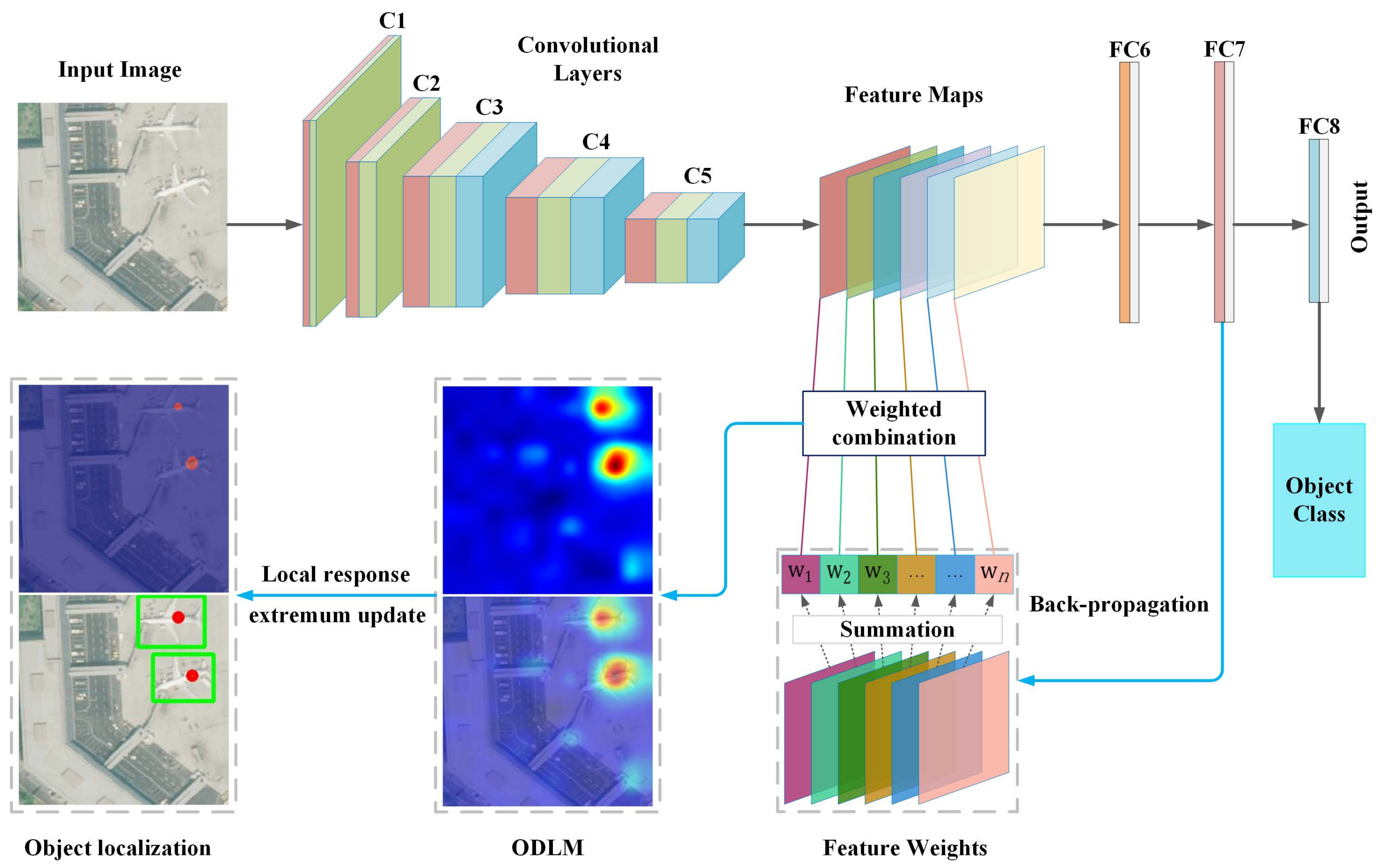
In this section, we evaluate the object localization performance based on the proposed framework. Generally, our proposed framework produces an ODLM by combining features from the convolutional and fully connected layers of a DCNN framework. When the feature from the last convolutional layer of AlexNet or VGG-16 is typically down-sampled by a pooling layer, the vector feature from the penultimate fully connected layer is typically extracted as an image feature presentation, and the vector feature from the last fully connected layer can be regarded as a class discriminative feature in a CNN model. Based on this understanding, we combine different fully connected layers with the last pooling or convolutional layer to generate the corresponding ODLMs. The resulting comparisons based on these foundations are then conducted to explore the localization performance.

4.2.1. Precision and Recall Evaluation

As introduced in Section 3, our proposed object localization method is closely related to the threshold parameter t. In general, the threshold parameter t is set to be 0.50, and the corresponding aircraft and oiltank localization results evaluated by the precision (P) and recall (R) are shown in Table 1 and Table 2, respectively. For convenience, we use “AF#C” to represent the localization results obtained by the ODLM when spreading the #-th fully connected layer feature to the last convolutional layer based on the AlexNet framework. Similarly, we use “AF#P” to represent the localization results obtained by the ODLM when spreading the #-th fully connected layer feature to the last pooling layer based on the AlexNet framework.
As shown in Table 1, AF8C achieves the best localization performance for the aircraft objects. However, the localization precision is as low as 32.02%, even the corresponding localization recall rate reaches 89.66%. The comprehensive performance of oiltank object localization is better than that of the aircraft. Specifically, the precision rates of the AF6C, AF7C, and AF8C are all above 70.00% and the corresponding recall rates are all above 75.00%. In Table 2, the precision of aircraft localization has been improved to 74.27% with a recall of 93.32% achieved by VF6P. In addition, the highest precision of oiltank localization by the VGG network reaches 92.84% with a relatively low precision of 70.40% achieved by VF7C. Taking Table 1 and Table 2 together, the object localization performance of the convolutional layer-based ODLMs is much better than that of pooling layer-based ones. Furthermore, we can always acquire recall rates higher than the corresponding precision rates for aircraft localization, as the t = 0.50 is too low to suppress the noise information in ODLMs. By contrast, the precision rates of oiltank localization generally show better performance than the corresponding recall rates, especially for the VGG-based model. An overall comparison between Table 1 and Table 2 indicates that the object localization performance based on the VGG model is much better than that based on AlexNet model, given that AlexNet is a shallow network while VGG is a much deeper network. Consequently, the VGG model shows stronger ability to distinguish objects from their backgrounds.

4.2.2. Threshold Analysis

The object localization performance may vary with the change of the threshold t. Table 3, Table 4, Table 5 and Table 6 show the object localization results based on different threshold values ranging from 0 to 0.99. Note that the aircraft and oiltank localization results based on the AlexNet framework are shown in Table 3 and Table 4, respectively. The results based on the VGG framework are shown in Table 5 and Table 6, respectively. In each column, the maximum precision and recall values are reported in bold.
As shown in Table 3, Table 4, Table 5 and Table 6, the localization precision rates improve along with the increment of threshold t while the corresponding recall rates decrease gradually. When comparing the convolutional and pooling layer-based ODLMs in Table 3, we can find that the recall rates acquired by the convolutional layer-based ODLMs (e.g., AF6C, AF7C, and AF8C) can significantly outperform the corresponding pooling layer-based ODLMs (e.g., AF6P, AF7P, and AF8P). To take a further investigation, we can see that most of the recall rates for aircraft localization are over 90% when the threshold t is less than 0.50 when using ODLMs based on AF6C, AF7C, and AF8C. However, the localization precision rates are much lower than the corresponding localization recall rates when the thresholds are set as small values because there are many local minimum response values appeared as noises in the ODLMs. Nevertheless, the pooling layer-based ODLMs can achieve higher localization precision than the convolutional layer-based ODLMs since the pooling operation can smooth the influence of noise response values. It is worth noting that, when setting the thresholds greater than 0.50, the aircraft localization precision rates achieved by AF7C and AF8C improve significantly even if the corresponding recall rates decrease to a certain extent. Specifically, for the AF7C and AF8C-based ODLMs, the localization precision rates are close to 70.00% while the corresponding recall rates remain above 75.00% when t = 0.90 . In addition, both the recall and precision rates with the threshold of 0.99 surpass 70.00% and 74.00%, respectively, indicating that the noise response information contained in the ODLM can be effectively suppressed by a high threshold.
The oiltank localization results based on AlexNet are shown in Table 4. Different from the result of aircraft localization, both the recall and precision achieved by the convolutional layer-based ODLMs (e.g., AF6C, AF7C, and AF8C) outperform the corresponding pooling layer-based ODLMs (e.g., AF6P, AF7P, and AF8P) when t > 0.10 . Furthermore, the AF6C-based ODLMs consistently achieve the best localization results that outperform those from AF7C- and AF8C-based ODLMs even under different threshold settings. It is interesting to find that the satisfactory overall performance of oiltank localization can be obtained by setting the threshold t around 0.50. For example, the precision and recall rates can reach 73.29% and 78.81%, respectively, which is consistent with Table 1. In addition, the maximum recall rate for aircraft localization based on AlexNet framework can reach 95.26% by AF6C as described in Table 3. The maximum recall rate for oiltank localization is 88.27% by AF6C, as shown in Table 4. These results can be achieved by setting the threshold t to be 0.0 or 0.10, which means the disregard of noise suppression.
The object localization results for aircraft and oiltank images based on the VGG framework are shown in Table 5 and Table 6, respectively. As can be seen from Table 5, the VGG model can produce the best recall rates by VF6C-based ODLMs under different thresholds. Typically, the VF6P-based ODLMs achieve the best precision rates when t 0.80 , which is similar to the phenomenon of AlexNet-based aircraft localization shown in Table 3. Note that the VF6C also achieves the highest localization precision when t 0.90 . By further observation, we can find that both VF7C and VF8C can achieve high recall rates for aircraft localization, where the lowest recall rate can reach 81.90%. This result verifies the stability of the VGG-based network for aircraft localization. That is, the ODLMs based on features of different fully connected layer can effectively indicate most of the aircraft locations in a remote sensing image.
As shown in Table 6, the best oiltank localization results are mainly achieved by VF7C and VF8C under different threshold levels. Specifically, the recall rate of 80.74% and precision rate of 90.57% can be obtained when the threshold is 0.30 for VF7C. With the same threshold of 0.30, the VF8C can also achieve similar recall and precision rates, i.e., 80.21% and 90.51%, respectively. In addition, the best recall rate of oiltank achieved by the VGG framework is 88.09%, as shown in Table 6, which is similar to that of the Alexnet-based result. The best aircraft localization recall achieved by the VGG framework is 98.28%, as shown in Table 5, which is 5.61% higher than that from the Alexnet-based framework.
In general, the precision rates typically decrease with the increment of corresponding recall values. The high localization recall can be acquired with a small threshold value, while the comparatively high localization precision can be achieved by setting a larger threshold t close to 1 for noise suppression. Thus, we can achieve different recall and precision rates based on our proposed dynamic threshold strategy.

4.2.3. Overall Performance

From Table 3, Table 4, Table 5 and 
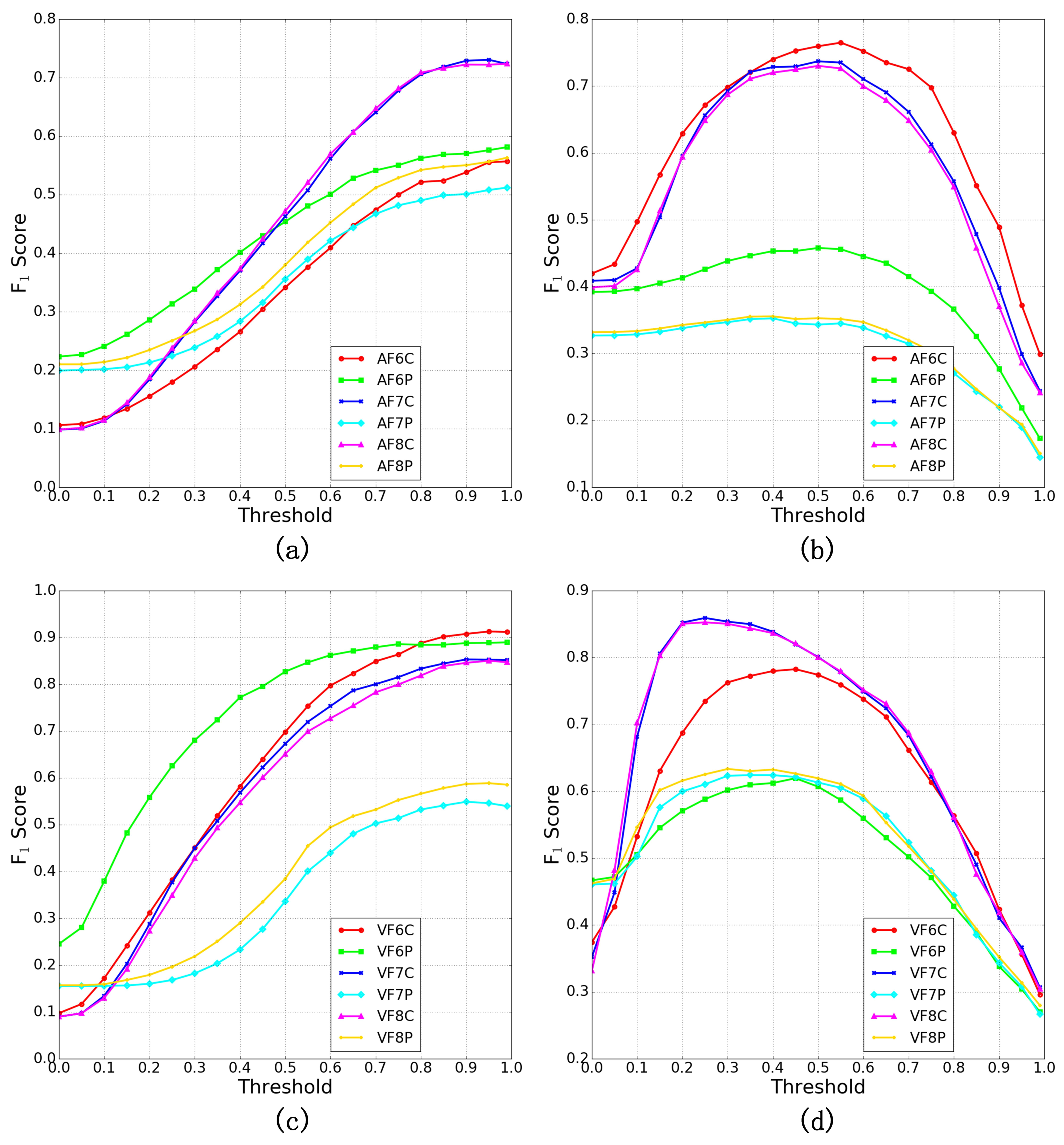
Table 6, we can find that the object localization performance varies significantly when spreading different fully connected layer features to the last convolutional or pooling layer. To further explore the comprehensive object localization performance of different feature layers, the F 1 -score measurement is employed to evaluate the object localization results of the different ODLM generalization schemes as shown in 
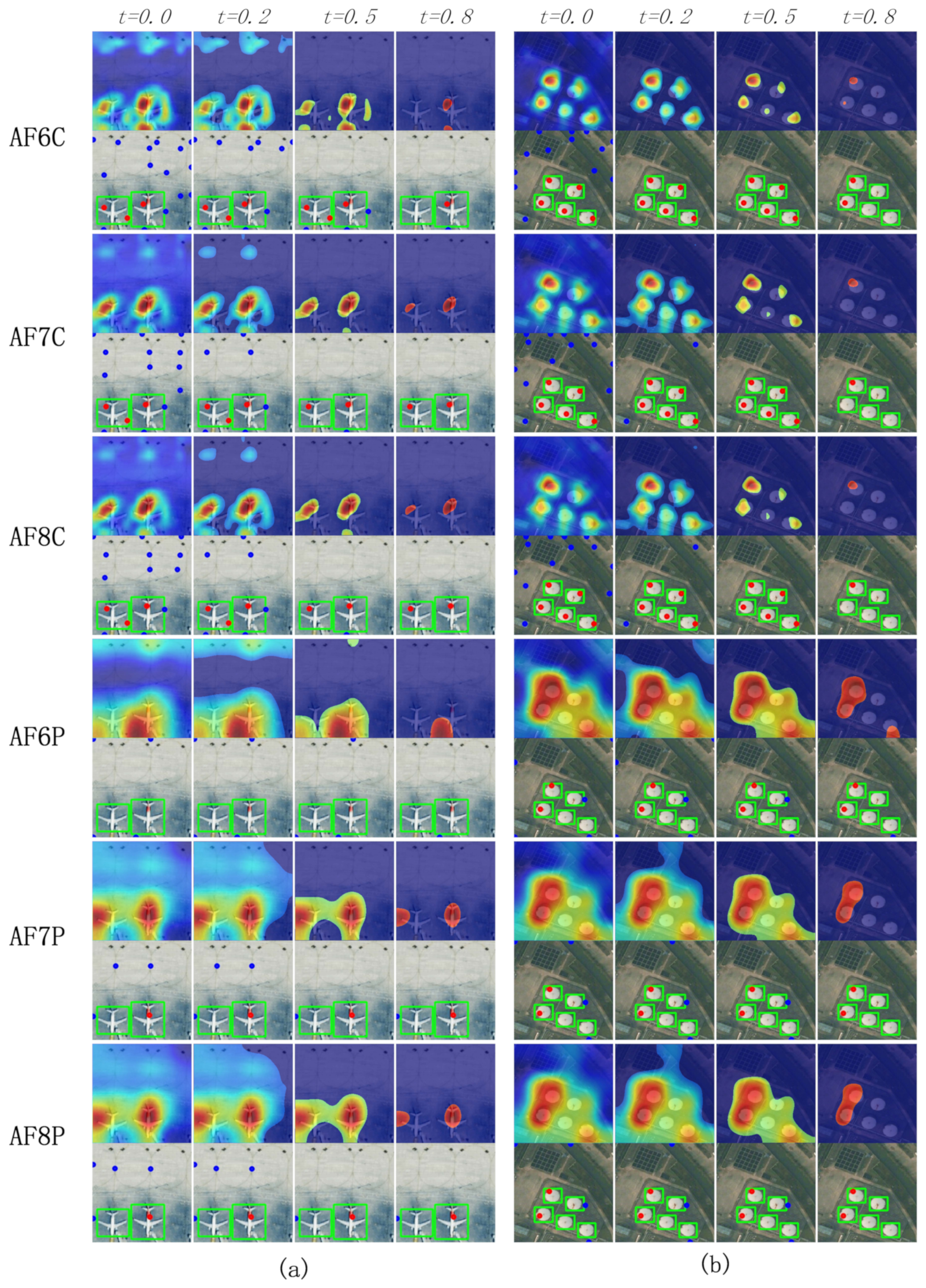
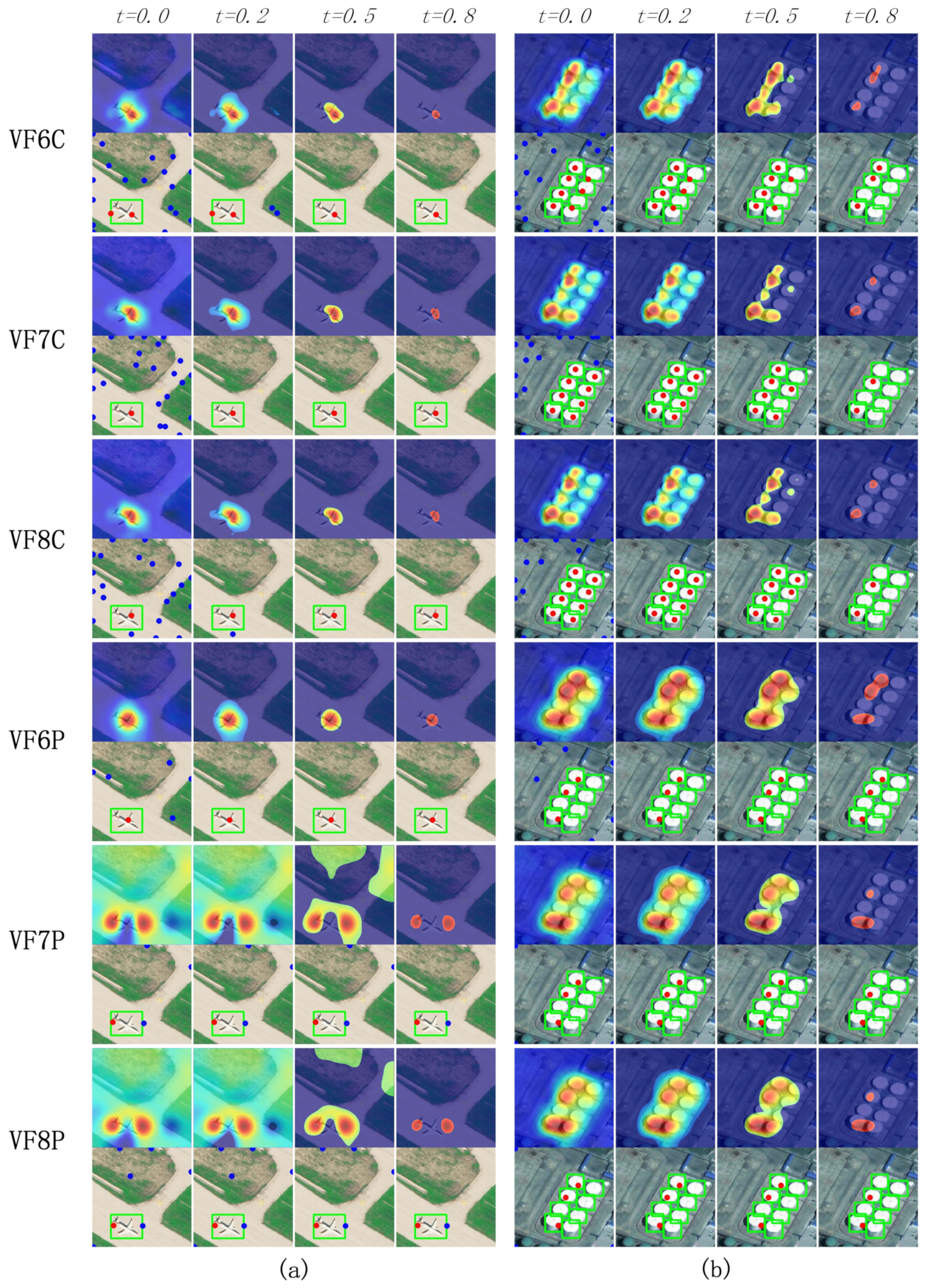
Figure 3. For a visual display, the ODLM samples from the test dataset are presented to further evaluate and understand the localization performance, as shown in Figure 4 and Figure 5.
As it can be seen, the curves in Figure 3 show similar variation trend for the objects with the same category. For example, the F 1 -score curves for oiltank localization shown in Figure 3b,d increase first and then decrease with the value increment of threshold t. However, the different ODLM generation schemes have different object localization performance even with the same threshold and CNN model. Specifically, for the AlexNet-based framework, the aircraft localization performance from AF6P, AF7P and AF8P are much better than those from AF6C, AF7C and AF8C when the threshold is below 0.20, as shown in Figure 3a. The similar result can also be observed in the VGG-based framework when the threshold t is smaller than 0.10 as shown in Figure 3c. This is because there is more light scattering noise response information contained in the ODLM when spreading the fully connected layer feature back to the last convolutional layer. By contrast, the response information is much smoother in the pooling layer-based ODLM which helps to improve the object localization precision, as shown in the first columns of Figure 4a and Figure 5a where the threshold is set as t = 0.0 , corresponding to the original ODLMs. Thus, more false locations are detected as positive ones through the proposed object location determination method, resulting in a negative influence on the localization precision performance. The locations represented by blue points in the first columns of Figure 4a and Figure 5a indicate this situation.
Nevertheless, with the increase of the threshold t, the overall performance of the convolutional layer-based ODLMs improves quickly for aircraft localization. Particularly, the F 1 -score curves of AF7C and AF8C are far above those of AF6P, AF7P, and AF8P when t 0.50 as shown in Figure 3a. Similarly, the F 1 -score curves of VF6C, VF7C, and VF8C significantly outperform those of VF7P and VF8P when t 0.20 as shown in Figure 3c. This is because the light scattering object location response information in the convolutional layer-based ODLMs is effectively suppressed by the threshold parameter as shown in Figure 4 and Figure 5. Consequently, the precision rate of aircraft localization by the convolutional layers improves quickly, which is consistent with the results in Table 3 and Table 5. Note that the curve of VF6P shows comparable performance with those of VF6C, VF7C, and VF8C. This result is mainly attributed to the high recall rate achieved by the VF6P-based ODLM as shown in Table 5. Nevertheless, the AF6C-based ODLM can achieve higher precision of aircraft localization when the threshold value goes beyond 0.8, resulting in better overall localization performance as shown in Table 5 and Figure 3c. On the other hand, the pooling layers in a CNN structure can easily lead to the loss of the spatial information for localizing local objects. Therefore, the pooling layer-based ODLMs (e.g., AF6P, AF7P, AF8P, VF7P, and VF8P) show weak localization ability if more than one aircraft appears in an image, as shown in Figure 4 and Figure 5.
As for the oiltank localization results, the F 1 -score curves of the convolutional feature-based ODLMs in general are all above those of the pooling layer-based ODLMs, as shown in Figure 3b,d. This indicates that the convolutional feature-based ODLMs can achieve higher recall and precision for oiltank localization, which is consistent with the results from Table 4 and Table 6. Corresponding to the above observation, the ODLMs presented in Figure 4b and Figure 5b show that the convolutional layer-based ODLMs can effectively recognize the location of each oiltank, while the pooling layer-based ODLMs tend to discriminate the regions of all oiltank locations as a whole. As a result, the oiltank localization performance of the convolutional layer-based ODLMs is much better than that of the pooling layer-based ODLMs. Specifically, though the noise response information is scattered over the background areas in the original ODLMs, the most salient regions can indicate the locations of oiltanks, allowing the oiltanks in an image to be effectively recognized and localized. Furthermore, it is interesting to find that the F 1 -score curves produced by the features from the last two fully connected layers always show the same performance, i.e., the he VF7C and VF8C shown in Figure 3d. The same phenomenon can also be observed in Figure 3a–c. A potential explanation is that the features from the last two fully connected layers can be trained well to represent the semantic content of a scene image. Comparatively, the feature from the shallower fully connected layer are immediately produced by the feature from the last convolutional layer. Thus, the combination of the features from the shallower fully connected layer and the last convolutional layer may lead to instability for the object’s position and semantics integration, i.e., AF6C and VF6C for aircraft and oiltank localization, respectively. Therefore, the ODLMs generated by features from the deep fully connected layers show better stability for object localization.
Note that there are an unexpected number of oiltanks in a remote sensing image, as shown in Figure 4b and Figure 5b. These oiltanks may appear at any location in an image and vary in scale and distribution density. These properties pose challenges to our proposed weakly supervised object localization method. Consequently, the degrees of response information may change for different oiltanks in an image. This effect is normal because the proposed weakly supervised object localization framework is merely constructed on the basis of a remote sensing image scene classifier of a CNN model. Moreover, the CNN classifier may focus on parts of the object regions in an image. As a result, the recall rate is high and the precision rate is much lower with a small noise threshold value. Similarly, the precision rate becomes high while the recall rate declines sharply as the threshold value increases. Thus, the F 1 -score curve rises at first and then drops sharply with the change of threshold values, which is different from the F 1 -score curves of aircraft localization. Nevertheless, the F 1 -score curves show that the proposed method can retain high comprehensive localization performance when the threshold values are approximately 0.5 for AlexNet-based and 0.3 for VGG-based localization schemes, as shown in Figure 3b,d, respectively. It is actually a balance between the localization precision and recall rates. In addition, these results are also consistent with those shown in Table 4 and Table 6.
Generally, the convolutional layer-based ODLMs show much better object localization abilities, as reflected in Table 3, Table 4, Table 5 and Table 6 and Figure 3, Figure 4 and Figure 5 since the ODLMs can effectively discriminate different objects and their backgrounds in a remote sensing image, as shown in Figure 4 and Figure 5. This capability ensures high recall rates while using a small threshold value for noise response information suppression, which is consistent with the results shown in Table 3, Table 4, Table 5 and Table 6. Specifically, Figure 3 shows that both the AlexNet and VGG framework can achieve excellent performance for aircraft localization with t 0.80 . In addition, satisfactory oiltank localization results can be obtained by setting the threshold between 0.30 and 0.50 for different CNN models.

4.2.4. Performance Comparison

Comparison of different networks: Table 7 and Table 8 show the best object localization performance measured by F 1 -score with the corresponding precision, recall, noise oppression parameter, distance error (DE), and the accuracy of image classification ( P c ) achieved by the employed AlexNet and VGG frameworks, respectively. The corresponding ODLMs and object localization results are also shown in Figure 6. As shown in Table 7, the F 1 -score of aircraft localization achieved by AlexNet-based framework reaches 73.06%. The F 1 -score of oiltank localization reaches 76.49%, which is 3.43% higher than that of the aircraft localization. Compared with AlexNet, the VGG-based framework shows much better localization performance with F 1 -scores of 91.56% and 85.97% for aircraft and oiltank localization, respectively. In fact, the shallower AlexNet framework mainly focuses on the local content while the deeper VGG framework can accurately localize different objects in an image to adapt to the semantic scene classification task. As shown in the first four lines of Figure 6, the VGG-based framework can localize most of the aircrafts even if they vary in appearance, scale, orientation, position, and spatial arrangement. The last column of the first four lines, which show the localization results for a small aircraft, also indicate the localization ability difference between different CNN models. Similarly, the oiltanks can also be localized with excellent performance, as shown in last column of lines 5–8 in Figure 6. Benefiting from the deep CNN architecture, the VGG-based framework achieved 18.5.% and 9.48% higher F 1 -scores than those of the AlexNet framework for aircraft and oiltank localization, respectively. However, both the AlexNet and VGG frameworks show weaknesses in localizing the mini-scale oiltanks, especially when they are adjacent to those oiltanks of large sizes. Nevertheless, both the AlexNet-based and VGG-based frameworks show remarkable effectivity in localizing the oiltanks, although there are an unexpected number of objects holding different positions, as shown in the last four lines of Figure 6.
Through aborative observation, we find that both the AlexNet-based and VGG-based frameworks tend to localize an oiltank by the borders between the object and its background. One possible explanation is that the trained CNN models tend to discriminate an oiltank from its backgrounds by focusing on the image content around object borders. Therefore, the AlexNet and VGG frameworks share approximate distance errors of oiltank localization, i.e., 18.27% and 15.64%, respectively. Similarly, the AlexNet-based framework localizes an aircraft by focusing on the aerofoil, tail, and head of an aircraft. Different from the aircraft localization results from AlexNet, the deeper CNN framework can recognize an aircraft with the location falling onto its body. Furthermore, the localized position by the VGG is much closer to the center of an aircraft’s annotated bounding box than that by AlexNet. As a result, the distance error of the aircraft localization by the VGG is much lower than that by AlexNet, as shown in Table 7 and Table 8. Furthermore, both the AlexNet and VGG frameworks achieve high accuracy of oiltank image scene classification, i.e., 93.20% and 98.00%, respectively. And the scene classification accuracy of aircraft images also reaches 94.40% and 95.20% by AlexNet and VGG, respectively. These results confirm that the extracted fully connected layer features can be powerful and class discriminative. Thus, the class information and spatial information could be effectively integrated while spreading the fully connected layer features back to the convolutional layers. Then, the excellent object localization performance can be achieved, which proves the rationality and effectivity of our proposed weakly supervised object localization framework.
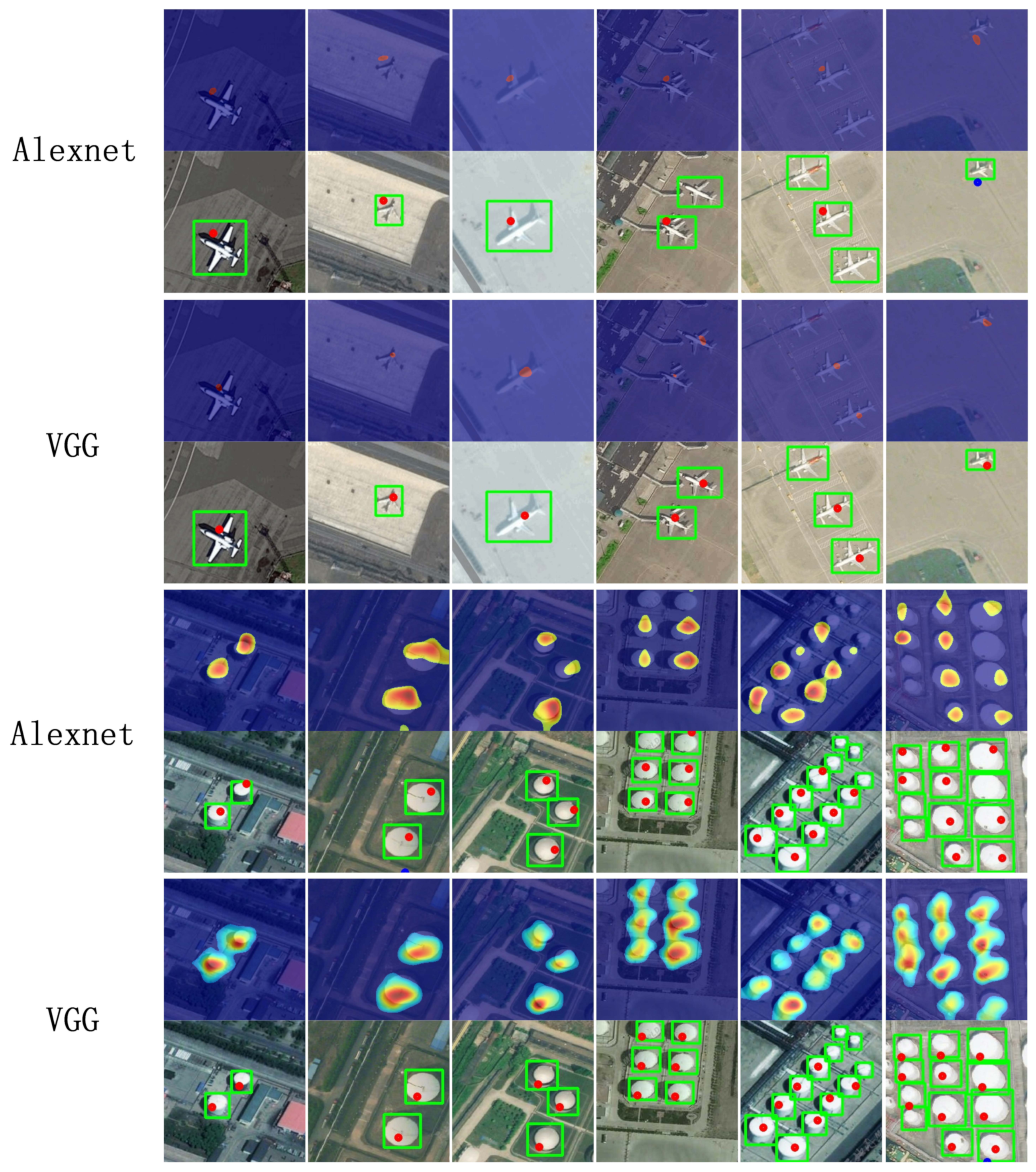
Comparison with existing methods: From above analyses, we can see that the proposed object localization method relies heavily on the quality of object discriminative localization map. Therefore, we compare our proposed method with the existing state-of-the-art (SOTA) class activation methods, including LayerCAM [81], XGradCAM [82], ScoreCAM [71], and ISCAM [83], etc. Specifically, we employ the VGG-based framework to generate ODLMs using different class activation methods. Then, the proposed dynamic updating method of local response extremum is utilized to obtain the object localization result. The quantitative results of object localization using different methods are presented in Table 9. As can be seen, our proposed method achieves the highest on F 1 -scores for both aircraft and oiltank localization. XGradCAM [82] typically propagates the class score at classification layer to the convolutional layer and generates class-related ODLMs. Thus, they achieve approximate performance of aircraft localization. LayerCAM [81] utilizes pixel-wise weights to integrate the convolutional features and generates an ODLM that can indicate the key parts of an object. However, the pixel-wise integration strategy can make the discriminative region of an object presented with scattered components, yielding massive noise and resulting in low aircraft localization precision, i.e., 52.17% and 10.22% for aircraft and oiltank, respectively. Score-CAM [71] and its improved version ISCAM [83] generate ODLMs by a linear combination of weights and activation maps, which can suppress the noise information. Thus, the ISCAM achieves the 91.31% of F 1 -score for aircraft localization. Nevertheless, our proposed method obtains comparable F 1 -score (91.56%) of aircraft localization. When it comes to the oiltank object localization, the compared methods observe sharp declines of localization performance. By contrast, our presented method can consistently outperform the compared methods on F 1 -score, precision, and recall, showing the strong stability of object localization ability of our proposed method.
Table 9. Comparison of object localization performance among different methods.
MethodAircraftOiltank
F1PRtDEF1PRtDE
LayerCAM [81]0.66280.52170.90830.9312.550.16610.10220.44310.7015.77
ScoreCAM [71]0.75310.65770.88070.998.840.66020.78250.57090.3917.33
XGradCAM [82]0.77250.66230.92660.879.540.28500.29780.27320.8913.43
ISCAM [83]0.91310.88330.94500.819.920.44830.44830.44830.6219.58
Ours0.91560.94500.88790.9814.860.85970.89120.83040.2315.64
The bold value in each column denotes the best result of the corresponding performance indicator.
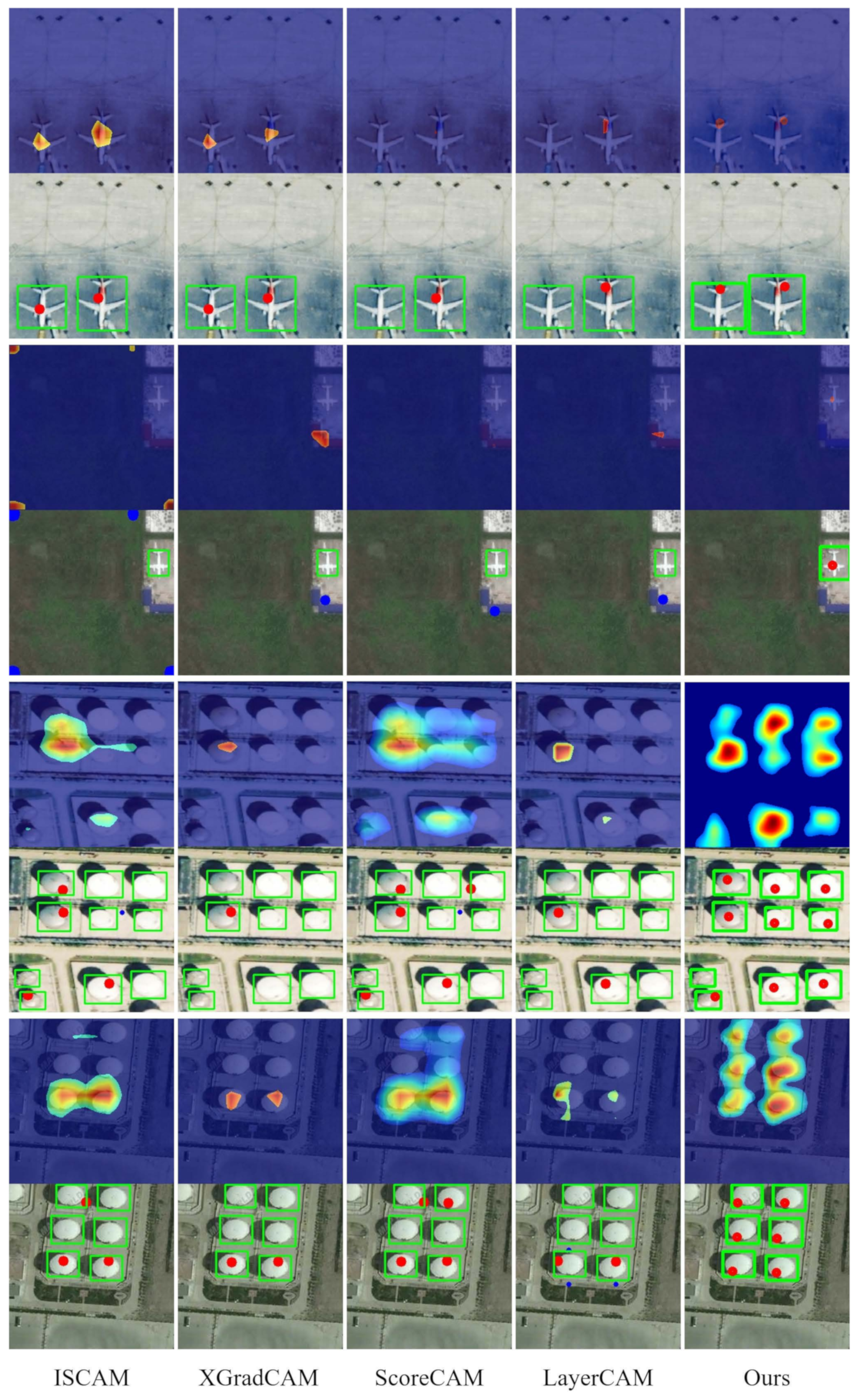
Figure 7 provides the intuitive visualization of object localization results. As can be seen from the first and second rows, the ISCAM, XGradCAM, and our proposed method can accurately localize the aircrafts in the image while the ScoreCAM and LayerCAM only focus on localizing one object in the image. Particularly, our proposed method can discriminate the aircraft of small size in the image while the compared methods fail to recognize the aircraft, as shown in the third and fourth rows of Figure 7. Consequently, our proposed method can achieve high aircraft localization precision that outperforms the compared methods as shown in Table 9. However, conventional class activation methods are usually designed to discriminate single object in an image. Thus, they tend to recognize the object areas as a whole, which makes the discrimination of multiple objects difficult as shown in the last four rows of Figure 7. By contrast, our proposed method tends to discriminate each object in the image, and thus, achieving significantly higher precision and recall for oiltank localization as shown in Table 9. Intuitively, conventional methods generate the ODLM only using the class score, which may cause the loss of information contained in the fully connected feature from classification layer. By contrast, our presented method backpropagates the class discriminative feature of the fully convolutional layer to the convolutional layer, which achieves the combination of class semantic and spatial information of objects. Therefore, the regions of multiple objects can be distinctly discriminated from theirs backgrounds, achieving high precision and recall of object localization.

5. Conclusions

In this work, we proposed a weakly supervised object localization framework to recognize objects using only image-level labels. To this end, semantic scene classification is conducted for the determination of object category. We backpropagate the class discriminative feature from the fully connected layer to the convolutional feature layer and generate an object discriminative localization map (ODLM) that can vividly indicate the salient regions of multiple objects in an image. In addition, a method of dynamic updating of local response extremum is proposed to further determine the location of different objects. Visualization results show that the ODLM established on the convolutional feature presents more accurate discriminative regions of objects than the pooling layer does. Extensive experiments and analyses show that the proposed framework can achieve satisfactory performance for the localization of remote sensing objects, i.e., aircrafts and oiltanks. In addition, the deeper CNN framework (VGG) can achieve significantly better localization result than the shallow one (AlexNet). Comparisons with the state-of-the-art methods indicate that our proposed method can achieve better performance and stability for the localization of multiple objects in remote sensing images. We hope that this work can provide new opportunities for further research concerning weakly supervised object localization and detection in remote sensing images. Our future work will focus on enhancing the framework and achieving the end-to-end method for weakly supervised object localization in remote sensing images.

Author Contributions

Conceptualization, Y.L. and X.Z.; methodology, Y.L., X.Z. and X.T.; software, Y.L. and Q.W.; validation, Y.L. and Q.W.; resources, Y.L., Q.W. and X.T.; writing—original draft preparation, Y.L.; writing—review and editing, Y.L. and X.Z.; supervision, X.Z. All authors have read and agreed to the published version of the manuscript.

Funding

This research received no external funding.

Conflicts of Interest

The authors declare no conflict of interest.

References

  1. Toth, C.; Jóźków, G. Remote sensing platforms and sensors: A survey. ISPRS J. Photogramm. Remote Sens. 2016, 115, 22–36. [Google Scholar] [CrossRef]
  2. Xiang, T.Z.; Xia, G.S.; Zhang, L. Mini-Unmanned Aerial Vehicle-Based Remote Sensing: Techniques, applications, and prospects. IEEE Geosci. Remote Sens. Mag. 2019, 7, 29–63. [Google Scholar] [CrossRef] [Green Version]
  3. Zou, Z.; Shi, Z.; Guo, Y.; Ye, J. Object detection in 20 years: A survey. arXiv 2019, arXiv:1905.05055. [Google Scholar]
  4. Gong, Y.; Xiao, Z.; Tan, X.; Sui, H.; Xu, C.; Duan, H.; Li, D. Context-Aware Convolutional Neural Network for Object Detection in VHR Remote Sensing Imagery. IEEE Trans. Geosci. Remote Sens. 2020, 58, 34–44. [Google Scholar] [CrossRef]
  5. Li, K.; Wan, G.; Cheng, G.; Meng, L.; Han, J. Object detection in optical remote sensing images: A survey and a new benchmark. ISPRS J. Photogramm. Remote Sens. 2020, 159, 296–307. [Google Scholar] [CrossRef]
  6. Ding, J.; Xue, N.; Xia, G.S.; Bai, X.; Yang, W.; Yang, M.Y.; Belongie, S.; Luo, J.; Datcu, M.; Pelillo, M.; et al. Object detection in aerial images: A large-scale benchmark and challenges. IEEE Trans. Pattern Anal. Mach. Intell. 2022, 1–18. [Google Scholar] [CrossRef]
  7. Sun, X.; Wang, P.; Yan, Z.; Xu, F.; Wang, R.; Diao, W.; Chen, J.; Li, J.; Feng, Y.; Xu, T.; et al. FAIR1M: A benchmark dataset for fine-grained object recognition in high-resolution remote sensing imagery. ISPRS J. Photogramm. Remote Sens. 2022, 184, 116–130. [Google Scholar] [CrossRef]
  8. Hoeser, T.; Kuenzer, C. Object Detection and Image Segmentation with Deep Learning on Earth Observation Data: A Review—Part I: Evolution and Recent Trends. Remote Sens. 2020, 12, 1667. [Google Scholar] [CrossRef]
  9. Hoeser, T.; Bachofer, F.; Kuenzer, C. Object Detection and Image Segmentation with Deep Learning on Earth Observation Data: A Review—Part II: Applications. Remote Sens. 2020, 12, 3053. [Google Scholar] [CrossRef]
  10. Cheng, G.; Han, J. A survey on object detection in optical remote sensing images. ISPRS J. Photogramm. Remote Sens. 2016, 117, 11–28. [Google Scholar] [CrossRef] [Green Version]
  11. Long, Y.; Gong, Y.; Xiao, Z.; Liu, Q. Accurate Object Localization in Remote Sensing Images Based on Convolutional Neural Networks. IEEE Trans. Geosci. Remote Sens. 2017, 55, 2486–2498. [Google Scholar] [CrossRef]
  12. Xia, G.S.; Bai, X.; Ding, J.; Zhu, Z.; Belongie, S.; Luo, J.; Datcu, M.; Pelillo, M.; Zhang, L. DOTA: A large-scale dataset for object detection in aerial images. In Proceedings of the 2018 IEEE Conference on Computer Vision and Pattern Recognition (CVPR), Salt Lake City, UT, USA, 18–23 June 2018; pp. 3974–3983. [Google Scholar]
  13. Wu, X.; Sahoo, D.; Hoi, S.C. Recent advances in deep learning for object detection. Neurocomputing 2020, 396, 39–64. [Google Scholar] [CrossRef] [Green Version]
  14. Wang, H.; Li, H.; Qian, W.; Diao, W.; Zhao, L.; Zhang, J.; Zhang, D. Dynamic pseudo-label generation for weakly supervised object detection in remote sensing images. Remote Sens. 2021, 13, 1461. [Google Scholar] [CrossRef]
  15. Shamsolmoali, P.; Chanussot, J.; Zareapoor, M.; Zhou, H.; Yang, J. Multipatch Feature Pyramid Network for Weakly Supervised Object Detection in Optical Remote Sensing Images. IEEE Trans. Geosci. Remote Sens. 2022, 60, 1–13. [Google Scholar] [CrossRef]
  16. Guo, G.; Han, J.; Wan, F.; Zhang, D. Strengthen learning tolerance for weakly supervised object localization. In Proceedings of the IEEE Conference on Computer Vision and Pattern Recognition (CVPR), Nashville, TN, USA, 20–25 June 2021; pp. 7403–7412. [Google Scholar]
  17. Zhang, D.; Han, J.; Cheng, G.; Yang, M.H. Weakly Supervised Object Localization and Detection: A Survey. IEEE Trans. Pattern Anal. Mach. Intell. 2021, 1–18. [Google Scholar] [CrossRef]
  18. Shao, F.; Chen, L.; Shao, J.; Ji, W.; Xiao, S.; Ye, L.; Zhuang, Y.; Xiao, J. Deep Learning for Weakly-Supervised Object Detection and Localization: A Survey. Neurocomputing 2022, 496, 192–207. [Google Scholar] [CrossRef]
  19. Waqas Zamir, S.; Arora, A.; Gupta, A.; Khan, S.; Sun, G.; Shahbaz Khan, F.; Zhu, F.; Shao, L.; Xia, G.S.; Bai, X. iSAID: A Large-scale Dataset for Instance Segmentation in Aerial Images. In Proceedings of the IEEE Conference on Computer Vision and Pattern Recognition Workshops (CVPRW), Long Beach, CA, USA, 16–20 June 2019; pp. 28–37. [Google Scholar]
  20. Oquab, M.; Bottou, L.; Laptev, I.; Sivic, J. Is object localization for free?—Weakly-supervised learning with convolutional neural networks. In Proceedings of the 2015 IEEE Conference on Computer Vision and Pattern Recognition (CVPR), Boston, MA, USA, 7–12 June 2015; pp. 685–694. [Google Scholar]
  21. Yu, H.; Li, G.; Zhang, W.; Huang, Q.; Du, D.; Tian, Q.; Sebe, N. The unmanned aerial vehicle benchmark: Object detection, tracking and baseline. Int. J. Comput. Vis. 2020, 128, 1141–1159. [Google Scholar] [CrossRef]
  22. Zhang, T.; Zhang, X.; Li, J.; Xu, X.; Wang, B.; Zhan, X.; Xu, Y.; Ke, X.; Zeng, T.; Su, H.; et al. Sar ship detection dataset (ssdd): Official release and comprehensive data analysis. Remote Sens. 2021, 13, 3690. [Google Scholar] [CrossRef]
  23. Ren, S.; He, K.; Girshick, R.; Sun, J. Faster r-cnn: Towards real-time object detection with region proposal networks. Adv. Neural Inf. Process. Syst. 2015, 28, 1–9. [Google Scholar] [CrossRef] [Green Version]
  24. Ding, J.; Xue, N.; Long, Y.; Xia, G.S.; Lu, Q. Learning roi transformer for oriented object detection in aerial images. In Proceedings of the 2019 IEEE Conference on Computer Vision and Pattern Recognition (CVPR), Long Beach, CA, USA, 15–20 June 2019; pp. 2849–2858. [Google Scholar]
  25. Dalal, N.; Triggs, B. Histograms of oriented gradients for human detection. In Proceedings of the 2005 IEEE Conference on Computer Vision and Pattern Recognition (CVPR), San Diego, CA, USA, 20–25 June 2005; Volume 1, pp. 886–893. [Google Scholar]
  26. Lowe, D.G. Distinctive Image Features from Scale-Invariant Keypoints. Int. J. Comput. Vis. 2004, 60, 91–110. [Google Scholar] [CrossRef]
  27. Li, F.; Perona, P. A Bayesian Hierarchical Model for Learning Natural Scene Categories. In Proceedings of the 2005 IEEE Conference on Computer Vision and Pattern Recognition (CVPR), San Diego, CA, USA, 20–25 June 2005; Volume 2, pp. 524–531. [Google Scholar]
  28. Cao, L.; Luo, F.; Chen, L.; Sheng, Y.; Wang, H.; Wang, C.; Ji, R. Weakly supervised vehicle detection in satellite images via multi-instance discriminative learning. Pattern Recognit. 2017, 64, 417–424. [Google Scholar] [CrossRef]
  29. Tang, Y.; Wang, X.; Dellandrea, E.; Masnou, S.; Chen, L. Fusing generic objectness and deformable part-based models for weakly supervised object detection. In Proceedings of the 2014 IEEE International Conference on Image Processing (ICIP), Paris, France, 27–30 October 2014; pp. 4072–4076. [Google Scholar]
  30. Wang, W.; Wang, Y.; Chen, F.; Sowmya, A. A weakly supervised approach for object detection based on soft-label boosting. In Proceedings of the 2013 IEEE Workshop on Applications of Computer Vision (WACV), Clearwater Beach, FL, USA, 15–17 January 2013; pp. 331–338. [Google Scholar]
  31. Deselaers, T.; Alexe, B.; Ferrari, V. Weakly supervised localization and learning with generic knowledge. Int. J. Comput. Vis. 2012, 100, 275–293. [Google Scholar] [CrossRef] [Green Version]
  32. Shi, Z.; Hospedales, T.M.; Xiang, T. Bayesian joint topic modelling for weakly supervised object localisation. In Proceedings of the 2013 IEEE International Conference on Computer Vision (ICCV), Sydney, Australia, 1–8 December 2013; pp. 2984–2991. [Google Scholar]
  33. Sikka, K.; Dhall, A.; Bartlett, M. Weakly supervised pain localization using multiple instance learning. In Proceedings of the 2013 10th IEEE International Conference and Workshops on Automatic Face and Gesture Recognition (FG), Shanghai, China, 22–26 April 2013; pp. 1–8. [Google Scholar]
  34. Siva, P.; Russell, C.; Xiang, T. In defence of negative mining for annotating weakly labelled data. In Proceedings of the European Conference on Computer Vision (ECCV), Florence, Italy, 7–13 October 2012; pp. 594–608. [Google Scholar]
  35. Wang, L.; Meng, D.; Hu, X.; Lu, J.; Zhao, J. Instance annotation via optimal bow for weakly supervised object localization. IEEE Trans. Cybern. 2017, 47, 1313–1324. [Google Scholar] [CrossRef] [PubMed]
  36. Shi, Z.; Hospedales, T.M.; Xiang, T. Bayesian joint modelling for object localisation in weakly labelled images. IEEE Trans. Pattern Anal. Mach. Intell. 2015, 37, 1959–1972. [Google Scholar] [CrossRef] [Green Version]
  37. Hoai, M.; Torresani, L.; De la Torre, F.; Rother, C. Learning discriminative localization from weakly labeled data. Pattern Recognit. 2014, 47, 1523–1534. [Google Scholar] [CrossRef]
  38. Gokberk Cinbis, R.; Verbeek, J.; Schmid, C. Multi-fold mil training for weakly supervised object localization. In Proceedings of the 2014 IEEE Conference on Computer Vision and Pattern Recognition (CVPR), Columbus, OH, USA, 23–28 June 2014; pp. 2409–2416. [Google Scholar]
  39. Han, J.; Zhang, D.; Cheng, G.; Guo, L.; Ren, J. Object Detection in Optical Remote Sensing Images Based on Weakly Supervised Learning and High-Level Feature Learning. IEEE Trans. Geosci. Remote Sens. 2015, 53, 3325–3337. [Google Scholar] [CrossRef] [Green Version]
  40. Zhou, P.; Zhang, D.; Cheng, G.; Han, J. Negative Bootstrapping for Weakly Supervised Target Detection in Remote Sensing Images. In Proceedings of the 2015 IEEE International Conference on Multimedia Big Data (BigMM), Beijing, China, 20–22 April 2015; pp. 318–323. [Google Scholar]
  41. Zhang, D.; Han, J.; Cheng, G.; Liu, Z.; Bu, S.; Guo, L. Weakly Supervised Learning for Target Detection in Remote Sensing Images. IEEE Geosci. Remote Sens. Lett. 2015, 12, 701–705. [Google Scholar] [CrossRef]
  42. Krizhevsky, A.; Sutskever, I.; Hinton, G.E. Imagenet classification with deep convolutional neural networks. In Proceedings of the Advances in Neural Information Processing Systems (NeurIPS), Lake Tahoe, NV, USA, 3–6 December 2012; pp. 1097–1105. [Google Scholar]
  43. Simonyan, K.; Zisserman, A. Very deep convolutional networks for large-scale image recognition. arXiv 2014, arXiv:1409.1556. [Google Scholar]
  44. Szegedy, C.; Liu, W.; Jia, Y.; Sermanet, P.; Reed, S.; Anguelov, D.; Erhan, D.; Vanhoucke, V.; Rabinovich, A. Going deeper with convolutions. In Proceedings of the 2015 IEEE Conference on Computer Vision and Pattern Recognition (CVPR), Boston, MA, USA, 7–12 June 2015; pp. 1–9. [Google Scholar]
  45. He, K.; Zhang, X.; Ren, S.; Sun, J. Deep Residual Learning for Image Recognition. In Proceedings of the 2016 IEEE Conference on Computer Vision and Pattern Recognition (CVPR), Las Vegas, NV, USA, 27–30 June 2016; pp. 770–778. [Google Scholar]
  46. Huang, G.; Liu, Z.; Van Der Maaten, L.; Weinberger, K.Q. Densely connected convolutional networks. In Proceedings of the 2017 IEEE Conference on Computer Vision and Pattern Recognition (CVPR), Honolulu, HI, USA, 21–26 July 2017; pp. 4700–4708. [Google Scholar]
  47. Hu, J.; Shen, L.; Sun, G. Squeeze-and-excitation networks. In Proceedings of the 2018 IEEE Conference on Computer Vision and Pattern Recognition (CVPR), Salt Lake City, UT, USA, 18–23 June 2018; pp. 7132–7141. [Google Scholar]
  48. Shen, Y.; Ji, R.; Zhang, S.; Zuo, W.; Wang, Y. Generative adversarial learning towards fast weakly supervised detection. In Proceedings of the 2018 IEEE Conference on Computer Vision and Pattern Recognition (CVPR), Salt Lake City, UT, USA, 18–23 June 2018; pp. 5764–5773. [Google Scholar]
  49. Tang, P.; Wang, X.; Wang, A.; Yan, Y.; Liu, W.; Huang, J.; Yuille, A. Weakly supervised region proposal network and object detection. In Proceedings of the European Conference on Computer Vision (ECCV), Munich, Germany, 8–14 September 2018; pp. 352–368. [Google Scholar]
  50. Shen, Y.; Ji, R.; Wang, Y.; Wu, Y.; Cao, L. Cyclic guidance for weakly supervised joint detection and segmentation. In Proceedings of the 2019 IEEE Conference on Computer Vision and Pattern Recognition (CVPR), Long Beach, CA, USA, 15–20 June 2019; pp. 697–707. [Google Scholar]
  51. Li, X.; Kan, M.; Shan, S.; Chen, X. Weakly supervised object detection with segmentation collaboration. In Proceedings of the 2019 IEEE Conference on Computer Vision and Pattern Recognition (CVPR), Long Beach, CA, USA, 15–20 June 2019; pp. 9735–9744. [Google Scholar]
  52. Gao, Y.; Liu, B.; Guo, N.; Ye, X.; Wan, F.; You, H.; Fan, D. C-midn: Coupled multiple instance detection network with segmentation guidance for weakly supervised object detection. In Proceedings of the 2019 IEEE International Conference on Computer Vision (ICCV), Seoul, Korea, 27 October–2 November 2019; pp. 9834–9843. [Google Scholar]
  53. Chen, Z.; Fu, Z.; Jiang, R.; Chen, Y.; Hua, X.S. Slv: Spatial likelihood voting for weakly supervised object detection. In Proceedings of the 2020 IEEE Conference on Computer Vision and Pattern Recognition (CVPR), Seattle, WA, USA, 13–19 June 2020; pp. 12995–13004. [Google Scholar]
  54. Durand, T.; Thome, N.; Cord, M. Weldon: Weakly supervised learning of deep convolutional neural networks. In Proceedings of the 2016 IEEE Conference on Computer Vision and Pattern Recognition (CVPR), Las Vegas, NV, USA, 27–30 June 2016; pp. 4743–4752. [Google Scholar]
  55. Zhu, Y.; Zhou, Y.; Ye, Q.; Qiu, Q.; Jiao, J. Soft proposal networks for weakly supervised object localization. In Proceedings of the 2017 IEEE International Conference on Computer Vision (ICCV), Venice, Italy, 22–29 October 2017; pp. 1841–1850. [Google Scholar]
  56. Bilen, H.; Vedaldi, A. Weakly supervised deep detection networks. In Proceedings of the 2016 IEEE Conference on Computer Vision and Pattern Recognition (CVPR), Las Vegas, NV, USA, 27–30 June 2016; pp. 2846–2854. [Google Scholar]
  57. Uijlings, J.R.; Van De Sande, K.E.; Gevers, T.; Smeulders, A.W. Selective search for object recognition. Int. J. Comput. Vis. 2013, 104, 154–171. [Google Scholar] [CrossRef] [Green Version]
  58. Zitnick, C.L.; Dollár, P. Edge boxes: Locating object proposals from edges. In Proceedings of the European Conference on Computer Vision (ECCV), Zurich, Switzerland, 6–12 September 2014; pp. 391–405. [Google Scholar]
  59. Zhang, F.; Du, B.; Zhang, L.; Xu, M. Weakly Supervised Learning Based on Coupled Convolutional Neural Networks for Aircraft Detection. IEEE Trans. Geosci. Remote Sens. 2016, 54, 5553–5563. [Google Scholar] [CrossRef]
  60. Zhou, B.; Khosla, A.; Lapedriza, A.; Oliva, A.; Torralba, A. Learning deep features for discriminative localization. In Proceedings of the 2016 IEEE Conference on Computer Vision and Pattern Recognition (CVPR), Las Vegas, NV, USA, 27–30 June 2016; pp. 2921–2929. [Google Scholar]
  61. Selvaraju, R.R.; Cogswell, M.; Das, A.; Vedantam, R.; Parikh, D.; Batra, D. Grad-CAM: Visual explanations from deep networks via gradient-based localization. In Proceedings of the 2017 IEEE International Conference on Computer Vision (ICCV), Venice, Italy, 22–29 October 2017; pp. 618–626. [Google Scholar]
  62. Xiao, Z.; Long, Y.; Li, D.; Wei, C.; Tang, G.; Liu, J. High-resolution remote sensing image retrieval based on CNNs from a dimensional perspective. Remote Sens. 2017, 17, 725. [Google Scholar] [CrossRef] [Green Version]
  63. Zhang, X.; Wei, Y.; Feng, J.; Yang, Y.; Huang, T.S. Adversarial complementary learning for weakly supervised object localization. In Proceedings of the 2018 IEEE Conference on Computer Vision and Pattern Recognition (CVPR), Salt Lake City, UT, USA, 18–23 June 2018; pp. 1325–1334. [Google Scholar]
  64. Zhang, X.; Wei, Y.; Kang, G.; Yang, Y.; Huang, T. Self-produced guidance for weakly-supervised object localization. In Proceedings of the European Conference on Computer Vision (ECCV), Munich, Germany, 8–14 September 2018; pp. 597–613. [Google Scholar]
  65. Choe, J.; Shim, H. Attention-based dropout layer for weakly supervised object localization. In Proceedings of the 2019 IEEE Conference on Computer Vision and Pattern Recognition (CVPR), Long Beach, CA, USA, 15–20 June 2019; pp. 2219–2228. [Google Scholar]
  66. Xue, H.; Liu, C.; Wan, F.; Jiao, J.; Ji, X.; Ye, Q. Danet: Divergent activation for weakly supervised object localization. In Proceedings of the 2019 IEEE International Conference on Computer Vision (ICCV), Seoul, Korea, 27 October–2 November 2019; pp. 6589–6598. [Google Scholar]
  67. Yang, S.; Kim, Y.; Kim, Y.; Kim, C. Combinational class activation maps for weakly supervised object localization. In Proceedings of the IEEE Winter Conference on Applications of Computer Vision (WACV), Snowmass Village, CO, USA, 1–5 March 2020; pp. 2941–2949. [Google Scholar]
  68. Mai, J.; Yang, M.; Luo, W. Erasing integrated learning: A simple yet effective approach for weakly supervised object localization. In Proceedings of the 2020 IEEE Conference on Computer Vision and Pattern Recognition (CVPR), Seattle, WA, USA, 13–19 June 2020; pp. 8766–8775. [Google Scholar]
  69. Chattopadhay, A.; Sarkar, A.; Howlader, P.; Balasubramanian, V.N. Grad-cam++: Generalized gradient-based visual explanations for deep convolutional networks. In Proceedings of the IEEE Winter Conference on Applications of Computer Vision (WACV), Lake Tahoe, NV, USA, 12–15 March 2018; pp. 839–847. [Google Scholar]
  70. Ramaswamy, H.G. Ablation-cam: Visual explanations for deep convolutional network via gradient-free localization. In Proceedings of the IEEE Winter Conference on Applications of Computer Vision (WACV), Snowmass Village, CO, USA, 1–5 March 2020; pp. 983–991. [Google Scholar]
  71. Wang, H.; Wang, Z.; Du, M.; Yang, F.; Zhang, Z.; Ding, S.; Mardziel, P.; Hu, X. Score-CAM: Score-weighted visual explanations for convolutional neural networks. In Proceedings of the 2020 IEEE Conference on Computer Vision and Pattern Recognition Workshops (CVPRW), Seattle, WA, USA, 14–19 June 2020; pp. 24–25. [Google Scholar]
  72. Diba, A.; Sharma, V.; Pazandeh, A.; Pirsiavash, H.; Van Gool, L. Weakly supervised cascaded convolutional networks. In Proceedings of the 2017 IEEE Conference on Computer Vision and Pattern Recognition (CVPR), Honolulu, HI, USA, 21–26 July 2017; pp. 914–922. [Google Scholar]
  73. Wei, Y.; Shen, Z.; Cheng, B.; Shi, H.; Xiong, J.; Feng, J.; Huang, T. Ts2c: Tight box mining with surrounding segmentation context for weakly supervised object detection. In Proceedings of the European Conference on Computer Vision (ECCV), Munich, Germany, 8–14 September 2018; pp. 434–450. [Google Scholar]
  74. Shwartz-Ziv, R.; Tishby, N. Opening the black box of deep neural networks via information. arXiv 2017, arXiv:1703.00810. [Google Scholar]
  75. Xia, G.S.; Hu, J.; Hu, F.; Shi, B.; Bai, X.; Zhong, Y.; Zhang, L.; Lu, X. AID: A benchmark data set for performance evaluation of aerial scene classification. IEEE Trans. Geosci. Remote Sens. 2017, 55, 3965–3981. [Google Scholar] [CrossRef] [Green Version]
  76. Cheng, G.; Han, J.; Lu, X. Remote sensing image scene classification: Benchmark and state of the art. Proc. IEEE 2017, 105, 1865–1883. [Google Scholar] [CrossRef] [Green Version]
  77. Cheng, G.; Xie, X.; Han, J.; Guo, L.; Xia, G.S. Remote Sensing Image Scene Classification Meets Deep Learning: Challenges, Methods, Benchmarks, and Opportunities. IEEE J. Sel. Top. Appl. Earth Obs. Remote Sens. 2020, 13, 3735–3756. [Google Scholar] [CrossRef]
  78. Maas, A.L.; Hannun, A.Y.; Ng, A.Y. Rectifier nonlinearities improve neural network acoustic models. In Proceedings of the 2013 International Conference on Machine Learning (ICML), Atlanta, GA, USA, 16–21 June 2013; pp. 1–6. [Google Scholar]
  79. He, K.; Zhang, X.; Ren, S.; Sun, J. Delving Deep into Rectifiers: Surpassing Human-Level Performance on ImageNet Classification. In Proceedings of the 2015 IEEE International Conference on Computer Vision (ICCV), Santiago, Chile, 7–13 December 2015; pp. 1026–1034. [Google Scholar]
  80. Murray, N.; Perronnin, F. Generalized max pooling. In Proceedings of the 2014 IEEE Conference on Computer Vision and Pattern Recognition (CVPR), Columbus, OH, USA, 23–28 June 2014; pp. 2473–2480. [Google Scholar]
  81. Jiang, P.T.; Zhang, C.B.; Hou, Q.; Cheng, M.M.; Wei, Y. LayerCAM: Exploring hierarchical class activation maps for localization. IEEE Trans. Image Process. 2021, 30, 5875–5888. [Google Scholar] [CrossRef]
  82. Fu, R.; Hu, Q.; Dong, X.; Guo, Y.; Gao, Y.; Li, B. Axiom-based grad-cam: Towards accurate visualization and explanation of cnns. arXiv 2020, arXiv:2008.02312. [Google Scholar]
  83. Naidu, R.; Ghosh, A.; Maurya, Y.; Kundu, S.S. IS-CAM: Integrated Score-CAM for axiomatic-based explanations. arXiv 2020, arXiv:2010.03023. [Google Scholar]
Figure 1. Framework of object Localization in Weakly Labeled Remote Sensing Images based on the VGG network.
Remotesensing 14 03230 g001
Figure 2. Scene images of each class. Two samples from the following classes are shown: (a) aircraft; (b) oiltank; (c) basketball court; (d) bridge; (e) building; (f) container; (g) fishpond; (h) footbridge; (i) forest; (j) greenhouse; (k) intersection; (l) airport; (m) overpass; (n) parking lot; (o) agricultural; (p) playground; (q) residential; (r) river; (s) ship; (t) solar power area; (u) square; (v) tennis court; (w) water; (x) wharf, and (y) workshop.
Remotesensing 14 03230 g002
Figure 3. Overall object localization performance by F 1 -score measurement. (a) Aircraft localization based on AlexNet. (b) Oiltank localization based on AlexNet. (c) Aircraft localization based on VGG. (d) Oiltank localization based on VGG.
Remotesensing 14 03230 g003
Figure 4. AlexNet-based ODLMs and the corresponding object localization results with different thresholds. (a) Aircraft localization for different feature layers. (b) Oiltank localization for different feature layers. The green boxes are manually annotated object bounding boxes. The detected true positive locations are indicated with red points while the false positive locations with blue points.
Remotesensing 14 03230 g004
Figure 5. VGG-based ODLMs and the corresponding object localization results with different thresholds. (a) Aircraft localization for different feature layers. (b) Oiltank localization for different feature layers. The green boxes are manually annotated object bounding boxes. The detected true positive locations are indicated with red points while the false positive locations with blue points.
Remotesensing 14 03230 g005
Figure 6. Object localization results based on the AlexNet and VGG frameworks. The green boxes are manually annotated object bounding boxes. The detected true positive locations are represented by red points while the false positive locations are represented by blue points.
Remotesensing 14 03230 g006
Figure 7. Object localization results among different methods. The detected true positive locations are indicated with red points while the false positive locations with blue points.
Remotesensing 14 03230 g007
Table 1. Object localization performance based on AlexNet ( t = 0.5 ).
ClassAF6CAF6PAF7CAF7PAF8CAF8P
PRPRPRPRPRPR
Aircraft0.21110.89220.34700.65520.31290.89010.25850.57110.32020.89660.27800.5991
Oiltank0.73290.78810.55330.39050.71060.76530.41180.29420.70410.75830.42200.3030
Table 2. Object localization performance based on VGG ( t = 0.5 ).
ClassVF6CVF6PVF7CVF7PVF8CVF8P
PRPRPRPRPRPR
Aircraft0.54470.97200.74270.93320.51800.95910.21860.73060.49230.96120.26120.7263
Oiltank0.87610.69350.77810.4970.92840.70400.79010.50090.92630.70400.79830.5061
Table 3. Localization performance of aircrafts with different thresholds of t based on AlexNet.
Threshold (t)0.000.100.200.300.400.500.600.700.800.900.99
AF6CP0.05620.06320.08470.11560.15530.21110.27070.33950.41280.47900.5714
R0.95260.95260.94830.94400.92460.89220.83840.78660.70910.61420.5431
AF6PP0.13450.14760.18290.22810.28880.34700.40790.47060.51430.55130.5964
R0.65730.65730.65730.65730.65730.65520.64870.63790.62070.59050.5668
AF7CP0.05200.06040.10240.16730.23310.31290.41410.51510.62750.69610.7432
R0.92030.92030.91380.90950.89870.89010.87280.8470.80600.76510.7047
AF7PP0.12010.12180.13030.15000.18750.25850.33770.40510.45260.48580.5249
R0.58620.58620.58620.58410.57970.57110.56030.55170.53450.51720.5000
AF8CP0.05210.06120.10460.16830.23530.32020.42150.52110.62690.68600.7460
R0.92670.92460.92460.91590.90300.89660.87930.85340.81470.76290.7026
AF8PP0.12670.12960.14500.17080.20990.27800.36400.44820.50280.53110.5753
R0.61420.61420.61420.61210.60990.59910.59700.59700.58840.57110.5517
The bold values in each column denote the best performance indicators under the corresponding threshold.
Table 4. Localization performance of oiltanks with different thresholds of t based on AlexNet.
Threshold (t)0.000.100.200.300.400.500.600.700.800.900.99
AF6CP0.27530.34590.49070.59390.67090.73290.80320.85680.90490.92230.9189
R0.88270.88270.87570.84760.82490.78810.70750.62870.48340.33270.1786
AF6PP0.38830.39790.43210.49130.53320.55330.55970.56670.57740.54640.5315
R0.39580.39580.39580.39580.39400.39050.36950.32750.26800.18560.1033
AF7CP0.26710.28340.45440.58900.66470.71060.74000.76380.77740.78760.7615
R0.87040.87040.86340.84060.80560.76530.68300.58320.43430.26620.1454
AF7PP0.32800.33160.35090.37550.40000.41180.42370.43890.45450.48800.4667
R0.32570.32570.32570.32220.31520.29420.28200.24520.19260.14190.0858
AF8CP0.26040.28320.45670.58780.65800.70410.73550.76610.78500.77220.7593
R0.85460.85460.84940.82660.79510.75830.66730.56220.42210.24340.1436
AF8PP0.33450.33810.35740.38140.40490.42200.43420.44270.45600.47930.4766
R0.32920.32920.32920.32400.31700.30300.28900.25040.19960.14190.0893
The bold values in each column denote the best performance indicators under the corresponding threshold.
Table 5. Localization performance of aircrafts with different thresholds of t based on VGG.
Threshold (t)0.000.100.200.300.400.500.600.700.800.900.99
VF6CP0.05130.09420.18510.29210.41360.54470.68250.77780.86210.91470.9446
R0.99140.99140.98920.98710.98060.97200.95910.93530.91590.90090.8815
VF6PP0.14080.23680.39480.53000.65420.74270.80790.85080.87870.90400.9215
R0.95470.95470.95470.95040.94180.93320.92460.90950.89010.87280.8599
VF7CP0.04720.07220.16890.29270.40230.51800.62790.71070.78370.84860.8822
R0.97840.97840.97410.97200.96770.95910.94180.91590.89010.85780.8233
VF7PP0.08670.08690.08970.10380.13820.21860.32350.41240.47390.52670.5545
R0.75220.75220.75220.75220.74780.73060.68750.64440.60780.57330.5259
VF8CP0.04710.06960.15890.27450.38060.49230.59320.68730.76450.83440.8776
R0.98280.98280.97840.97630.97200.96120.93970.90950.88150.85780.8190
VF8PP0.08780.08920.10190.12830.18070.26160.38070.44440.51040.56600.6009
R0.74350.74350.74350.74350.73490.72630.70470.66380.63580.60990.5711
The bold values in each column denote the best performance indicators under the corresponding threshold.
Table 6. Localization performance of oiltanks with different thresholds of t based on VGG.
Threshold (t)0.000.100.200.300.400.500.600.700.800.900.99
VF6CP0.24000.38760.59140.73620.81890.87610.90790.91360.92770.93980.9615
R0.85110.85110.82140.79160.74430.69350.62170.51840.40460.27320.1751
VF6PP0.40000.46040.58320.66950.73060.77810.79170.81500.81370.80790.8364
R0.56040.56040.55870.54640.52710.49740.43260.36250.29070.21370.1611
VF7CP0.22020.55800.86620.90570.91510.92840.93460.94440.94940.96130.9720
R0.88090.87570.83890.80740.77410.70400.62520.53590.39400.26090.1821
VF7PP0.39720.46370.66740.74450.77260.79010.80550.83210.84730.84830.8654
R0.54820.54820.54470.53590.52360.50090.46410.38180.30120.21540.1576
VF8CP0.20460.59000.87000.90510.91480.92630.93020.94210.95380.95630.9717
R0.87220.86690.83190.80210.77060.70400.63050.54120.39750.26800.1804
VF8PP0.39430.53430.69450.75670.78290.79830.81160.84520.84500.86900.8796
R0.55870.55870.55340.54470.53060.50610.46760.37300.29600.22070.1664
The bold values in each column denote the best performance indicators under the corresponding threshold.
Table 7. Best localization performance of F 1 -score measurement based on AlexNet.
ClassF1PRtDEPc
aircraft0.73060.73060.73060.9526.030.9440
oiltank0.76490.77520.75480.5518.270.9320
Table 8. Best localization performance of F 1 -score measurement based on VGG.
ClassF1PRtDEPc
aircraft0.91560.94500.88790.9814.860.9520
oiltank0.85970.89120.83040.2315.640.9800
Publisher’s Note: MDPI stays neutral with regard to jurisdictional claims in published maps and institutional affiliations.

