Partial Scene Reconstruction for Close Range Photogrammetry Using Deep Learning Pipeline for Region Masking

Abstract

3D reconstruction is a beneficial technique to generate 3D geometry of scenes or objects for various applications such as computer graphics, industrial construction, and civil engineering. There are several techniques to obtain the 3D geometry of an object. Close-range photogrammetry is an inexpensive, accessible approach to obtaining high-quality object reconstruction. However, state-of-the-art software systems need a stationary scene or a controlled environment (often a turntable setup with a black background), which can be a limiting factor for object scanning. This work presents a method that reduces the need for a controlled environment and allows the capture of multiple objects with independent motion. We achieve this by creating a preprocessing pipeline that uses deep learning to transform a complex scene from an uncontrolled environment into multiple stationary scenes with a black background that is then fed into existing software systems for reconstruction. Our pipeline achieves this by using deep learning models to detect and track objects through the scene. The detection and tracking pipeline uses semantic-based detection and tracking and supports using available pretrained or custom networks. We develop a correction mechanism to overcome some detection and tracking shortcomings, namely, object-reidentification and multiple detections of the same object. We show detection and tracking are effective techniques to address scenes with multiple motion systems and that objects can be reconstructed with limited or no knowledge of the camera or the environment.

1. Introduction

A 3D point cloud is a data structure that encapsulates geometric information (positions) of an object or a scene. It consists of a list of points. Each point has x, y, and z coordinates with optional color information; red, green, and blue (RGB) [1]. Point clouds have several use cases in various applications that span different fields such as medical, engineering, and computer graphics. For example, point clouds can be used at construction sites to measure and evaluate a construction project against original designs providing efficiency and accuracy over manual methods [1,2]. Another interesting use of point clouds is computer-aided design (CAD) model reconstruction or reverse engineering [3] to recover a 3D model of old mechanical parts. Additionally, there are many complex geometries and textures in nature such as trees and fruits that can be challenging to model directly using CAD toolsets. 3D reconstruction is a valuable technique to obtain realistic 3D objects from a sample which saves time over manual artistic design. A common method is to create a point cloud and then either use that point cloud directly, or convert it into another model, such as polygonal, subdivision, or spline-based. 3D reconstruction is used in game development and virtual and augmented realities to add the look and feel of complex objects [4,5]. For example, multiple museums allow visitors to take virtual tours and explore their artwork in the museum’s digital twin.

The use of 3D reconstruction has a promising future and will continue to grow.

Different tools (hardware and software) have been developed to acquire a 3D point cloud by sampling the surface locations of an object or a scene. The tools can be grouped into two main categories: active or passive sensors [6]. Active sensors act on the environment to collect location data, such as Light Detection and Ranging (LiDAR). LiDAR samples location points by emitting a light (laser) beam and measures the round trip time after hitting an object to compute the distance or the position relative to the light source [1]. A beam represents a single point, so to sample the full scene, the beam is moved both horizontally and vertically to sample the complete scene. LiDAR is a precise device that has some cost-effective solutions, but it is more likely to be expensive to achieve a high-precision 3D reconstruction. LiDAR is a common sensor equipped on self-driving cars to obtain a point cloud of the surrounding scene, often in coordination with other sensors that work in all weather conditions. The point cloud data is used by obstacle avoidance and path-following algorithms [7]. Passive sensors, such as monocular or binocular cameras, are used along with software tools to generate point clouds. This is referred to as the photogrammetry approach. The basic principle is to obtain two or more different views of the scene and then triangulate the locations between matching points. Figure 1 shows a reconstruction example where a point cloud is generated from a set of images by matching features in different views and then projecting those matching points from the 2D image locations back through space (using the inverse projection of the camera) to determine the location in 3D space.

The photogrammetric approach is software-oriented, relatively inexpensive, and it can be as accurate as active sensors in a controlled environment. The previous reconstruction example is an instance of a controlled turntable where the turntable facilitates the acquisition of images without the need of moving the camera providing various views of the object with controlled lighting and background. The turntable setup has been successful in various projects such as heritage preservation [8,9,10,11] and plant reconstruction [10]. However, the turntable introduces another challenge as the extracted features from the scene belong to at least two distinct motion systems, namely the background and the object.

For instance, moving objects or a rich environment (background with high-frequency information) may introduce ambiguous features [9]. In other words, feature ambiguity creates conflicts resulting in either duplicate points, inconsistent geometry, or missing points. Another reconstruction experiment, Figure 2, shows the result of feeding imagery of a dynamic environment of the same yellow truck. The end result is a partially reconstructed, deformed point cloud, and only a small portion of the images (cameras) were used and they were incorrectly positioned. The error can be reduced by placing a black or white (roughly featureless) background to guide the software to target the object’s features only as previously shown in Figure 1.

Prior research has shown, as described above, that turntable approaches can be used to do Structure from Motion (SfM) or reconstruct a point cloud for a target object. However, one current limitation of such work is the need for a static or ancillary background. In contrast, this work proposes using deep learning technology, to analyze visual data (images and videos) and automatically add a true featureless background. We argue that the current deep learning techniques can be used to extend the use of SfM software and allow reconstruction from existing videos that were made without reconstruction in mind. In this research, we take objects in uncontrolled dynamic environments and then use deep learning tools to transform the objects into a controlled environment for high-quality reconstruction. For instance, we show that the proposed pipeline would reconstruct the yellow truck using the uncontrolled imagery that is roughly equivalent to the yellow truck reconstruction using the controlled imagery. To achieve our goal, we built a deep learning detection and tracking pipeline using off-the-shelf neural networks (commonly used in security and surveillance applications) designed for close-range photogrammetry (turntable) reconstruction applications. In addition to a correction algorithm to improve object tracking as well as sampling and masking mechanism to separate the target object(s) from the scene. The pipeline is intended to relax some rigorous turntable constraints such as size and background. The pipeline is a preprocessing step to automatically isolate the target object(s) from the scene and place a blank (black) background to overcome current limitations. The pipeline is available online and supports multiple detection networks (algorithms), and it can be modified for other use cases.

2. Background

SfM is a complex, powerful technique to recover 3D scene structure from a set of images. However, it has limited performance in dynamic scenes. This section briefly describes the SfM pipeline, its limitations, and different techniques to address various dynamic scenarios.

Different SfM software systems follow roughly the same similar set of steps as shown in Figure 3. Incremental reconstruction is probably the most prominent methodology for SfM software systems [12,13]. It consists of two main phases: the feature correspondence search and incremental reconstruction. The first phase starts with feature extraction to find point features in the input images that have discriminative properties and are resilient to changes in lighting and object orientation [12] followed by feature matching. Feature matching relies on the uniqueness of objects and resiliency traits to find corresponding points between image pairs for the extracted features and uses them as the basis for identifying the camera transformation and point locations in the 3D space. Geometric verification is the last step in the first phase and the purpose is to calculate the relative transformation between image pairs. The next phase uses the correspondence information to build the 3D point cloud. Reconstruction initialization selects the best image pair as the seed for the final point cloud and incrementally adds new points from new images through image registration triangulation. The image registration deduces the camera position with respect to the available 3D points by solving the perspective-n-point problem (2D to 3D) followed by the triangulation step where it verifies the projection of a portion of the 3D points into the newly added image and expands the number of points by the new observed points in the registered 2D image. Finally, the bundle adjustment refines the camera positions and point locations simultaneously through a nonlinear least square formulation [14], which reduces error propagation from the image registration and triangulation and improves the final 3D reconstruction. The standard SfM technique implies a static environment where there is a single motion system that belongs to the camera. If there are two or more motion systems, point and camera location estimations may fail or generate unstable results [15]. Visual Odometry [16] and Visual SLAM [17] utilize the same principles as SfM but handle dynamic scenes to identify camera position and orientation for robotic and self-driving car tasks such as ego-motion and trajectory identification.

A straightforward method to handle separate motion is to ignore inconsistent (object) motion and maintain the static scene assumption so inconsistent features are treated as outliers. RANSAC [18] is a popular statistical approach to sample features and obtain a robust feature set to reconstruct the scene. It is commonly used in the standard SfM pipeline to ensure consistency and resiliency to outliers, but as the number of motion-independent features increases due to a dynamic scene, RANSAC becomes less effective. DynaSLAM [19] employs Masked RCNN to identify objects that do not belong to the scene and inpaint the region with a corresponding portion of the background from a previous frame. DysSLAM utilizes ORBSLAM2 [20] to track and estimate the camera position and orientation to correctly paint the dynamic regions. Similarly, DsSLAM [21] uses SegNet [22] to identify inconsistent motion of the scene along with ORB features [20,23] to track the features.

Previous approaches are valuable when the environment is mainly static; for example, a car or a person entering a scene during image collection. However, in a dynamic environment for autonomous cars or robots, moving objects need to be accounted for. Li et al. [14] introduce a semantic-based approach to account for moving objects and estimate 3D bounding boxes in an autonomous driving scenario using stereo vision. It combines the 2D bounding boxes of the objects generated by Faster RCNN [24] with a viewpoint classification network to roughly estimate the 3D bounding volume of the objects then it feeds the resulting information with ORB features to a tightly coupled bundle adjustment technique to ensure the temporal consistency between objects. Mask fusion [25] is another technique that takes advantage of semantic segmentation techniques using RCNN [26] to identify objects in a scene while also leveraging the depth information to track the different objects and ensure the geometrical consistency to track and reconstruct different objects. MID Fusion [27] is another similar technique to using geometric information of RGB-D (red, green, blue, and depth) cameras to improve object tracking with semantic segmentation. It tracks the objects based on other geometric features using ElasticFusion [28]. MID fusion also adds measurement (depth) uncertainties to ensure robust tracking and reconstruction with the semantic segmentation information. Stereo and RGB-D cameras are becoming more affordable and pervasive for use in robotics and similar applications where stereo cameras capture the 3D structure for each frame but they are not as ubiquitous as monocular cameras.

Monocular cameras are common sensors used with Structure from Motion software and they present more challenges to address when multiple objects are moving independently [29]. The main strategy to solve monocular dynamic scenes is to separate salient features along with their tracks based on their motion traits such that a group of features represents a single motion system. Given an accurate separation and an adequate number of features, the standard SfM techniques can be adopted to estimate their motion and structure [15]. Kundu et al. [30] introduce an incremental multibody visual SLAM that uses particle filters and bearing-only features (BOT) to integrate the different cues of a calibrated monocular camera to segment different motions and map the environment with reasonable accuracy in real-time. Ranftl et al. [31] introduce a two-stage approach to recover depth from a monocular camera in a dynamic scene. The first stage is to decompose the scene into different motion models with its epipolar geometry. The segmentation strategy is based on a convex relaxation of the Potts model [32] to fit different motion models to each scene component which allows the reconstruction of each component with an arbitrary scale followed by a scene assembly stage to deduce the correct scale and the placement of each component and recover the depth map. Google Brain and others [33,34] take advantage of the implicit representation of ego-motion and depth in a video sequence by explicitly introducing ego-motion, object motion, and depth as part of an unsupervised deep learning model setup where the model needs to deduce the depth and ego-motion to reduce the photogrammetric error between consecutive frames.

Point features are valuable to compute accurate measurements such as velocity and position. Many techniques rely on such features to perform motion segmentation for both monocular and stereo cameras [35,36,37], but low-level features are susceptible to motion blur and occlusion [15], which can significantly degrade measurement quality. Additionally, point-level features do not reflect semantics which in turn can over- or under-segment objects in the scene, while understanding a dynamic environment in terms of position and velocity of the surrounding through point-level computation or direct depth estimation is valuable for navigation, mapping, and other similar tasks, adding semantic information can elevate some of the issues and improve measurements based on point-level features and also add additional value for point-level feature output (point cloud). For instance, semantic-oriented methods [38] such as semantic segmentation are promising techniques that can reconstruct objects that have more semantic value and it adds additional constraints to improve the reconstruction quality. Even though semantic techniques are limited to pretrained priors [39], various techniques are being introduced to expand the possible priors with minimal modification such as transfer and few-shot learning [40,41].

3. Methodology

Close-range photogrammetry takes advantage of Structure from Motion or visual SLAM techniques to obtain a finely detailed point cloud by constraining the data collection phase by taking the photographs of an object in a controlled environment such as a turntable. This section introduces a semantics-based detection and tracking pipeline designed for photogrammetric tasks to convert a dynamic scene into multiple subscenes for each object that resembles a close-range photogrammetry-controlled environment.

Given a dynamic scene, Ş, of multiple objects, $O_1,O_2,\dots ,O_n$, where each object follows independent motion, $M_1,M_1,\dots ,M_n$, and each motion is a series of transformations, $t_{1,1},t_{1,2},\dots ,t_{n,m}$, (that is the transformation between two consecutive frames per object), the scene can be represented in a matrix form as shown in the equation below. Each row is a single frame and a single column is an object’s motion though time. A dynamic scene cannot be reconstructed directly using an SfM software system when the scene contains two or more independent motions.

$$Ş=\left[\begin{array}{cccc}{t}_{1,1}{O}_1& t_{1,2}{O}_2& \cdots & t_{1,n}{O}_n\\ t_{2,1}{O}_1& t_{2,2}{O}_2& \cdots & t_{2,n}{O}_n\\ ⋮& ⋮& \ddots & ⋮\\ t_{m,1}{O}_1& t_{m,2}{O}_2& \cdots & t_{m,n}{O}_n\end{array}\right]$$

The detection and tracking pipeline phase decomposes the scene, based on the visual appearance of an object, into a set of independent scenes where each independent scene is of a single object during the entire video. A single independent scene can be reconstructed by an SfM software system.

$$Ş=\left[\begin{array}{c}{t}_{1,1}\\ t_{2,1}\\ ⋮\\ t_{m,1}\end{array}\right]O_1,\left[\begin{array}{c}{t}_{1,2}\\ t_{2,2}\\ ⋮\\ t_{m,2}\end{array}\right]O_2,\cdots ,\left[\begin{array}{c}{t}_{1,n}\\ t_{2,n}\\ ⋮\\ t_{m,n}\end{array}\right]O_n$$

Our preprocessing pipeline consists of two components that use state-of-the-art convolutional neural networks (CNN); one for object detection and the other for object tracking. There are several models available for object detection, such as Single Shot Detection [42], You Only Look Once (YOLO) [43], RCNN [44], Fast RCNN [45], and Faster RCNN [24], and the models vary in their speed and accuracy.The pipeline uses Faster RCNN [24] as the default detection network due to its superior accuracy; however, any detection model from TensorFlow model zoo (https://github.com/tensorflow/models/blob/master/research/object_detection/g3doc/tf1_detection_zoo.md (accessed on 20 December 2018)) can be used. Similarly, object tracking relies on feature representation, which is a core component for many vision algorithms. However, it is the main goal to identify objects across multiple views, frames, or temporarily separated imagery. Many tracking algorithms define a similarity measure [46] between object representations in two successive frames to determine if they are the same or a different object.

As shown in Figure 4, the proposed framework processes the input imagery and removes the object background from the scene and saves all the different views of the objects with a black (featureless) background. The resulting imagery is then fed to the reconstruction software system and the output is a point cloud for each separate object detected with reduced irrelevant points. The detection and tracking pipeline effectively acts as a preprocessing step that removes irrelevant features before the construction process.

Robust detection networks such as (faster RCNN) can be sufficient for certain 3D scanning setups where only a single detectable object is present in the scene or multiple objects from different classes. However, misclassified or multiple objects of the same class (multiple chairs) would be grouped as the same object which acts as noise and degrades the reconstruction process. To overcome this, our pipeline uses an additional tracking layer to avoid these issues. The Simple Online and real-time tracking [47] (SORT) original formulation uses a Kalman filter and Hungarian algorithm to track multiple objects in real-time. Deep SORT [48,49], extends SORT to use visual traits for improved performance. Deep sort uses a convolutional neural network to extract the visual descriptors of the objects. Even though the network is trained on pedestrian images, the network tends to identify other objects as well, probably because of the Kalman filter [50]. Our pipeline uses Deep SORT since it tracks objects for longer times, handles occlusions, and reduces the number of identification switches and allows object re-identification.

The framework forms the two detection and tracking algorithms as a single entity. Our framework loads a video, then passes each frame to the detection network (faster RCNN by default) and splits the scene into separate objects. The detected objects are then passed to the tracking algorithm to match them to previously detected objects. The tracking algorithm will maintain the association between the different views of the same object during the video. Then each object can be reconstructed independently.

However, a common issue in tracking algorithms is that they tend to lose track of one or more objects and reidentify them as new ones [46]. The problem arises because an object in a frame does not meet the minimum similarity requirement, or matching score, with the view of the same object in the following frame, $t+1$, so the tracking algorithm treats them as different objects and generates new IDs for them. Even though some tracking algorithms, such as Deep SORT can recover from incorrect reidentification, there will be a period of time when the algorithm loses track of one or more objects. The loss of tracking directly impacts the number of views (frames) of the detected object, and since the SfM relies on the different views to triangulate the object points in space, the loss of tracking will probably reduce the reconstruction quality of that object.

In order to address the issue of incorrect reidentification, we introduce a correction algorithm to merge the objects that are more likely to be incorrectly reidentified by the tracking algorithm. The correction algorithm assumes that if an object disappears and a new object appears roughly in the same position in the following frame that it is the same object and they are merged. For consecutive frames, the algorithm first detects the disappearing objects, $\mathsf{\Gamma }$, which are those objects in frame t that disappeared in the following frame, $t+1$, given as the difference between the sets of object IDs, $O_t$, and $O_{t+1}$:

$$\mathsf{\Gamma }=O_t-O_{t+1}$$

and then computes which is the objects that appeared in frame $t+1$ and were not in frame t, using:

$$\mathsf{\Omega }=O_{t+1}-O_t$$

The merging step is computed by maximizing the overlap between the first and second sets, as shown below

$$arg\underset{i,j}{max}\frac{{\mathsf{\Gamma }}_i\cap {\mathsf{\Omega }}_j}{{\mathsf{\Gamma }}_i\cup {\mathsf{\Omega }}_j}$$

where ${\mathsf{\Gamma }}_i$ is the region occupied by object i in the $\mathsf{\Gamma }$ set and ${\mathsf{\Omega }}_j$ the region occupied by object j in the set $\mathsf{\Omega }$.

This initial formulation of the merge addresses the tracking algorithm losing track of objects. The merge tool assumes the detection network can identify the objects in all frames and therefore it has a unique ID. However, usually, a detection network can miss objects in two or more consecutive frames as well as detect an object multiple times which adds limitations to the merge tool. However, the merge tool can be generalized to overcome this. First, it is allowed to run the tool multiple times over different time spans or frame gaps which will fix the loss of detection period and reidentification as well. Second, the merge tool can run on a 0 frame gap which allows it to identify duplicate detections of the same object. An overlap threshold is used to make sure that only point sets with a large overlap are considered the same object and that the entire scene does not get merged.

As seen in Figure 4, the pipeline is a composition of software utilities that are designed to work in a sequential fashion. The pipeline is developed in Python and it is composed of four main utilities. The first utility is the detection tool that is used to read an input video and feed it to the detection network frame by frame. The output of the tool is the object bounding boxes along each frame. The tool is designed to load roughly any detection network from the TensorFlow pretrained model zoo or any other trained model on a custom dataset. The second tool is the modified version of Deep SORT codebase (https://github.com/nwojke/deep_sort (accessed on 8 April 2019)) that is designed to accept the output of the detection tool and generate IDs for the different objects and maintain them throughout the video. The output of the tracking tool is meta-information about the objects appearing in the video, their bounding boxes, and their IDs. The merge tool is used to combine the different objects that are more likely to be reidentified incorrectly and it outputs a new set of meta-information. Finally, the sampling and masking tool uniformly samples a number of frames for each object, based on its tracking ID and gives it a featureless black background using the bounding box. Each object can then independently be sent to the SfM software to generate a point cloud. Because each object is scanned independently any issues caused by the separate motion of each object are resolved. The four software tools formulate the proposed system as a single entity to preprocess input video.

4. Experimental Setup and Results

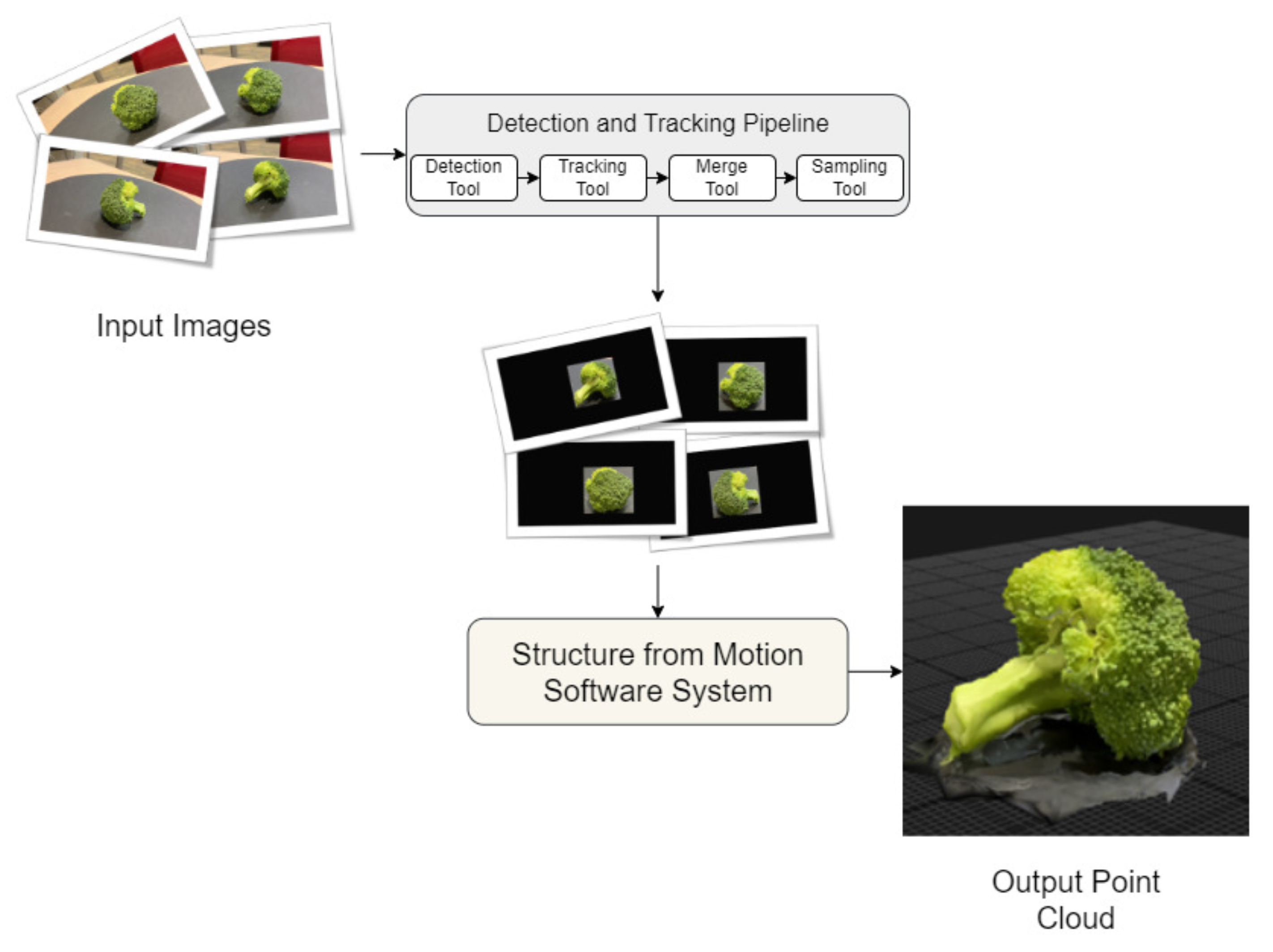
The detection and tracking pipeline and Structure from Motion software present a framework to utilize existing tools and technologies to recover or reconstruct partial regions of a scene based on the objects present in the scene. The pipeline incorporates a correction mechanism to merge incorrectly reidentified objects during tracking to maintain the object tracking for a longer time. The framework introduces a strategy to decompose a dynamic scene, which may not be reconstructed using SfM software only, into multiple static only sub-scenes by detecting and tracking objects, separating them from the main scene, then feeding them to SfM software and recovering the point clouds.

We designed experiments to evaluate the reconstruction quality of SfM software systems with and without the proposed pipeline. First, we determine the reconstruction accuracy of a point cloud using a controlled SfM setup (turntable with black background) by comparing measurements on the point cloud to measurements obtained from the actual object. Then we compare the reconstruction integrity or deformation with and without the pipeline against the controlled SfM reconstruction.

4.1. Dataset

Structure from Motion software can produce a 3D point cloud (3D geometry) of an object by finding matching points between different views in a scene and obtaining the 3D position of points. A turntable is a common inexpensive setup with a black background to generate multiple views of an object for reconstruction (controlled environment) where the camera remains stationary, and the object rotates in front of the camera using the rotating table. The black background makes it easier for the reconstruction software to identify object points, rather than the background, which increases quality. We use this setup to collect scenes of different objects by recording short videos of a complete revolution of the objects at 4 K resolution and 60 frames per second to obtain as many features as possible and reduce blurring. The recording device is the rear camera of an iPad Pro 4th generation with a resolution of $3840\times 3024$. The recording speed and resolution are the only camera properties changed during the recordings, the remaining settings are left as the default, in order to evaluate the reconstruction with roughly no recording constraints.

Another set of short videos was recorded using the turntable for a complete revolution without the black background (uncontrolled environment). For this, we assume that we have no calibration information for the camera which would be the case when using a third-party recording. These recordings represent an uncontrolled dynamic scene where the object follows a different coordinate system other than the background, similar to the controlled setup, but the rich background introduces a set of features that is more likely to affect the object reconstruction negatively. The video series of the uncontrolled environment is being used to evaluate the efficacy of the detection and tracking pipeline as a preprocessing stage before SfM reconstruction. An additional video is recorded of the truck and the car together to evaluate the construction of multiple objects and the impact of the correction mechanism. The video is recorded with the same device but at 30 frames per second and the frame resolution is $1280\times 720$.

In our experiments, we used 5 objects that are represented in a common object in context (COCO) dataset [51], namely two miniature cars, a miniature airplane, broccoli, and a banana. The detection network is trained on the COCO dataset. The COCO dataset contains $1.5$ million items that span 91 different objects such as people, cars, and airplanes over 80 categories such as animals, vehicles, and accessories. Figure 5 shows the different objects in the controlled (Ctrl), the uncontrolled (Unctrl) environment, and masked (Msk), which is the result of our framework.

An additional video is recorded using the same camera settings of a checkerboard to calibrate the camera [52] for the controlled environment. MATLAB™is used to calibrate the camera from a sampled set of frames.

Table 1. Camera calibration report using MATLAB™.

	Fx [pix]	Fy [pix]	Cx	Cy	K1	K2	K3	P1	P2
Mean	2.9 × 10${}^3$	3.9 × 10${}^3$	1.9 × 10${}^3$	2.4 × 10${}^3$	0.06	0.26	0.00	0.00	0.00
SD	30.05	56.61	7.66	71.75	0.01	0.04	0.00	0.00	0.00

shows the camera intrinsic parameters determined using MATLAB™. The F_x and F_y are the focal length measured in pixels. C_x and C_y are the calibrated center or principal points offsets measured in pixels. K₁ to K₃ are radial distortion coefficients, also P₁ and P₂ are the tangential distortion coefficients. It is more likely calibration information varies from the product specifications due to the uncontrolled camera settings or manufacturing defects.

4.2. Evaluation

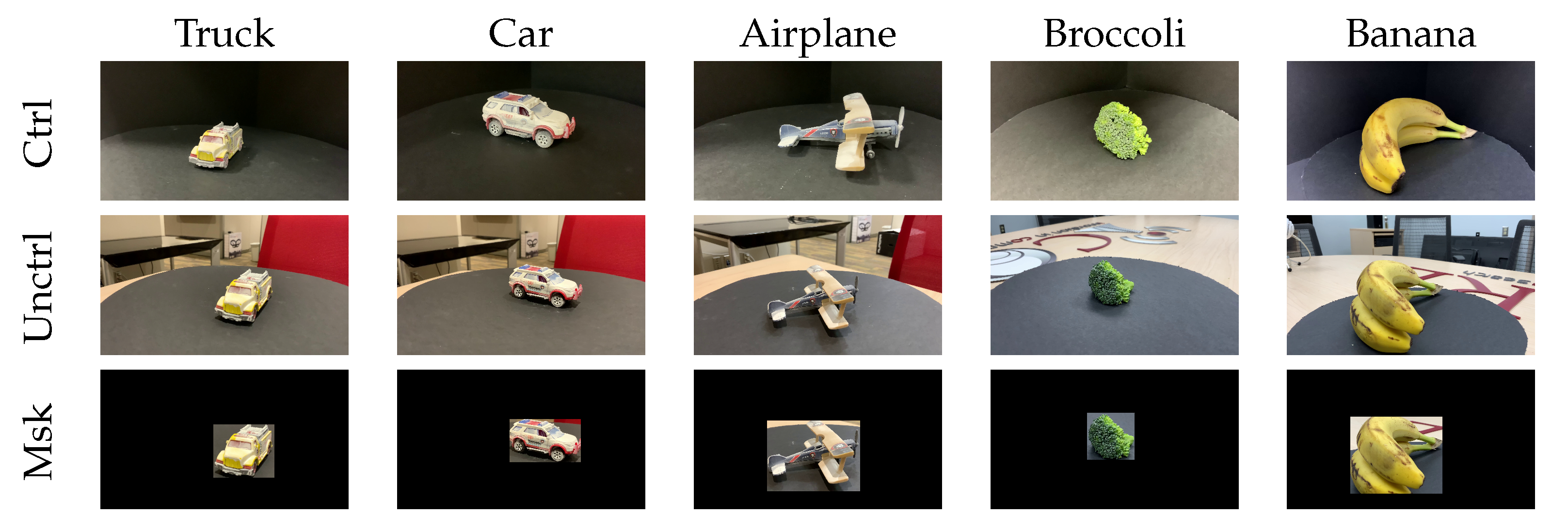
SfM utilities are powerful tools to reconstruct geometry or measure distances accurately. Our research is more concerned with the reconstruction of geometry for an arbitrary scene since measurement tools such as scaling markers or control points may not be available. In other words, we evaluate the reconstruction of an arbitrary video of an object and measure how it would be aligned with and without the detection and tracking pipeline as if it was recorded in a controlled environment. The experimental setup produces four different point clouds for each object, a raw point cloud, a masked point cloud, a controlled point cloud, and a reference point cloud. The raw point cloud (uncontrolled environment) results from feeding 200 frames to the SfM software. The masked point cloud results from preprocessing the frames with our pipeline and then feeding the processed frames to the SfM software. The controlled point cloud results from feeding 200 frames from the controlled environment to the SfM software. The reference point cloud is a manually cleaned version of the output of the SfM software of the frames from the controlled environment. The reference point cloud is used to evaluate the quality of the other two point clouds.

Additionally, we use three different state-of-the-art SfM software (Agisoft metashape, Pix4d, and RealityCapture) with their default reconstruction settings to evaluate the effect of our pipeline on each software. Since each software system has their own proprietary algorithms to reconstruct the point cloud it will be challenging to define a common reference point cloud for all software systems. Instead, we evaluate the reconstruction quality of the masked and raw point clouds with respect to the software being used. For example, we generate the reference, masked, and raw point clouds for each software system.

Furthermore, we determine the reconstruction quality using two methods for each software system. First, we compare the measurements of reference point clouds with the actual measurements from the objects (truck, car, and airplane) used in the experiments. Second, we measure the alignment or the deformation of the masked and raw point clouds against the reference point clouds. Since the alignment process between masked and raw point clouds with the reference point cloud contains only rigid transformations, then the alignment quality would directly indicate the masked and raw point cloud quality.

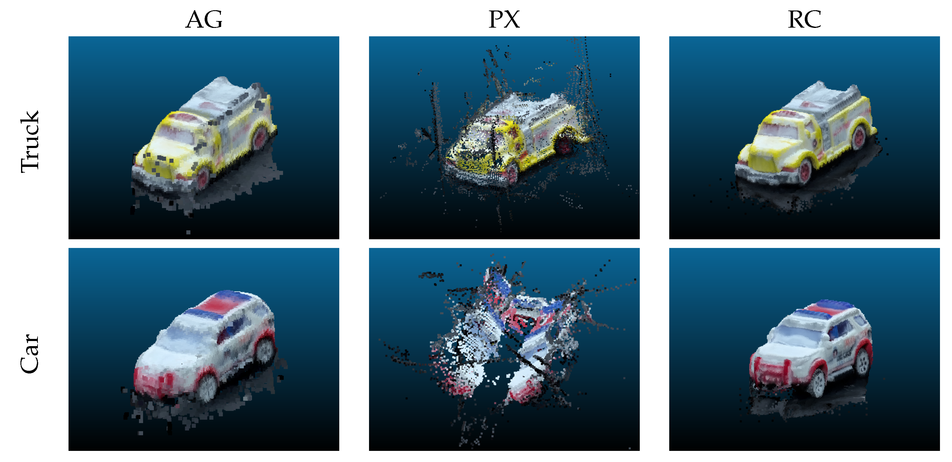
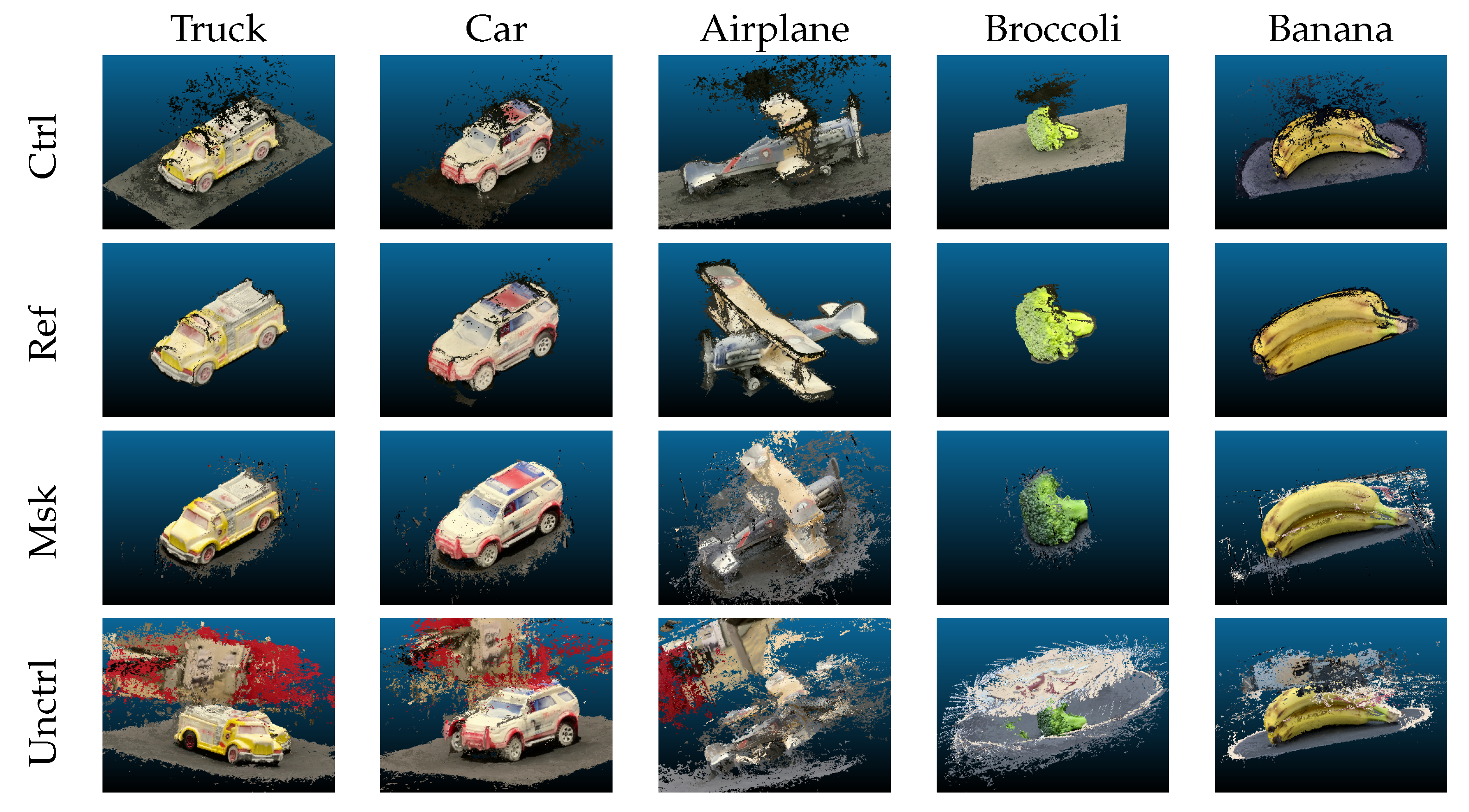
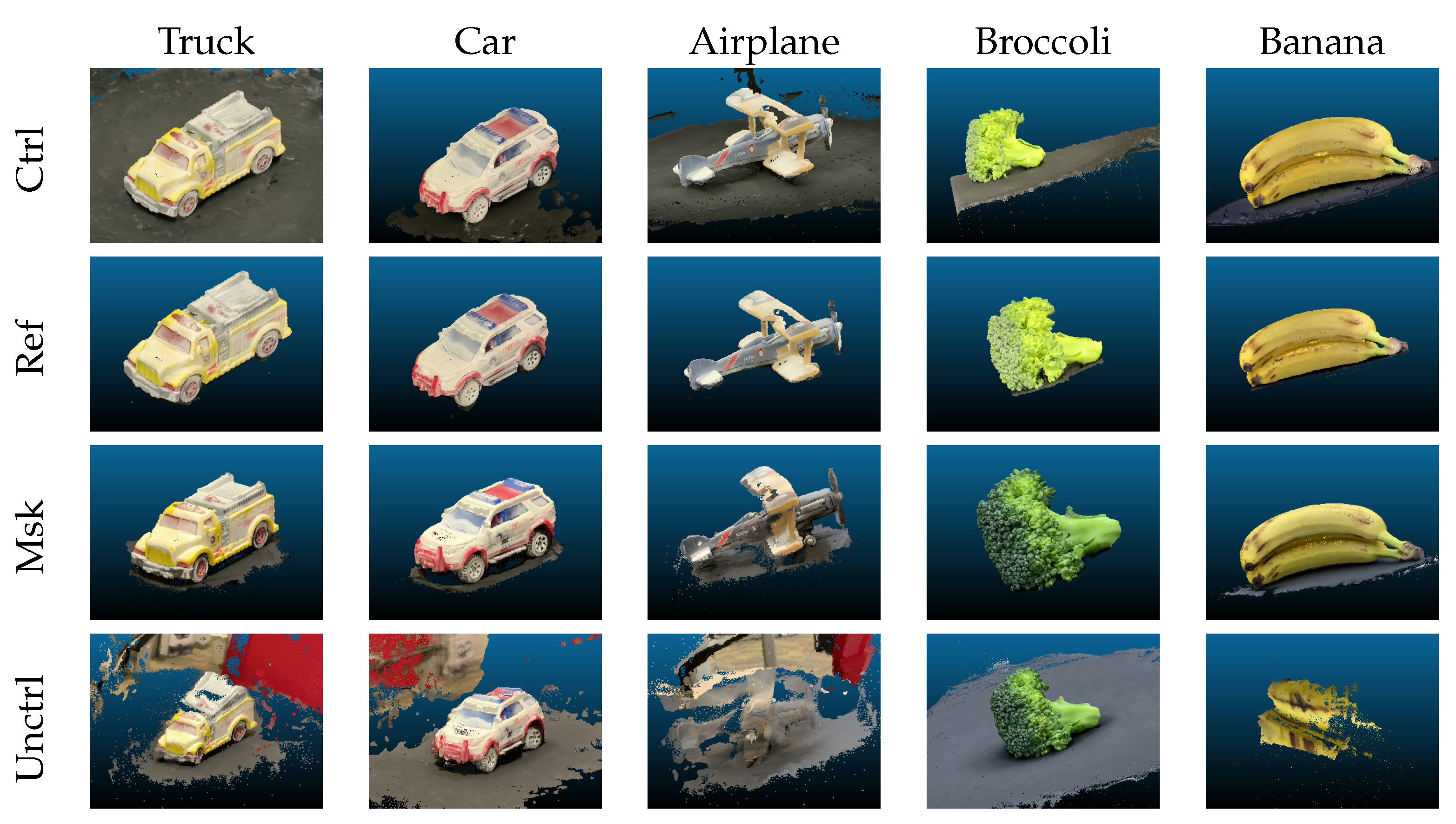
Figure 6, Figure 7 and Figure 8 show sample views of the different point clouds (masked, raw, and reference) per object. We use the short names Ctrl, Ref, Msk, Unctrl to refer to a controlled environment, reference, masked, and uncontrolled point clouds, respectively. It is clear that the SfM software was able to generate point clouds for a partial scene when using our pipeline, and it achieves accurate results compared to its corresponding raw point cloud where a large portion of the points are part of the background. Furthermore, the front of the yellow truck reconstruction using Agisoft, Pix4d, and RealityCapture is deformed without using our pipeline. For example, Agisoft constructed multiple portions of its front multiple times and skipped the rear part due to scene complexity, and in some cases, the raw point cloud is not usable.

However, the visual representation is not sufficient to quantify the reconstruction quality. As a point cloud consists of a list of 3D points where the number of points and the positions are used to compare and evaluate the reconstruction quality compared to the reference point cloud. We consider the number of points to be indicative of the signal-to-noise ratio or object points to scene points. As the ratio gets closer to 1, the generated points are more likely to be relevant to the target object.

Table 2. Number of points before and after noise removal.

Software	Agisoft		Pix4d		RealityCapture
Object	Noisy	Clean	Noisy	Clean	Noisy	Clean
Truck	455.8 K	133.1 K	245.3 K	217.3 K	688.6 K	225.2 K
Car	589.1 K	249.8 K	342.2 K	323.8 K	571.7 K	483.8 K
Airplane	1.7 M	470.2 K	427.3 K	337.3 K	1.6 M	405.3 K
Broccoli	1.1 M	233.9 K	392.8 K	285.4 K	700.37 K	319.4 K
Banana	1.7 M	664.4 K	426.6 K	380.2 K	1.2 K	676.6 K

shows the number of points for the reference objects before and after background (noise points) removal for each software. For instance, the yellow truck scene recorded 455.8 K points, but only 133 K points belong to the truck, roughly 1/4 of the scene points belong to the yellow truck, and the remaining points are irrelevant. SfM software adds additional background points, and that behavior is consistent between the different software and their scenes as shown in Table 2. The second metric is the average distance and standard deviation between two point clouds. Given two registered point clouds, registration is the process of transforming (scale, translate, or rotate) a target point cloud (scene) to align with a reference point cloud (object), and a distance measure can be computed to evaluate the geometrical (structural) quality of the target point cloud. Cloudcompare [53] uses a version of Hausdorff [54] distance between two sets of corresponding points. The modified version models the local surface near the points instead of computing the distances directly between the corresponding points of the reference and target point cloud to obtain reliable results. For instance, if the two point clouds are exactly the same, then the average distance and standard deviation should be 0, and both start to increase as one set of points deviate from its corresponding set of points, indicating the point cloud shape deformation.

However, the average distance and standard deviation are limited measures because during the reconstruction process we have no camera information (both intrinsic and extrinsic parameters) and we do not require any scaling markers. Hence each software system defines an arbitrary coordinate system to measure distances between points. The average distance and standard deviation, in this case, can show the deformation differences between the masked and raw point clouds only if the same reference point cloud is used. However, it may not translate to other point clouds of the same object because each software system uses an arbitrary unit in its internal coordinate system.

In order to fix this issue, we converted all of the units to millimeters and then compare results across systems. This allows us to use the average distance and standard deviation to evaluate the deformation of the point clouds independent of the software used. To convert to millimeters, we physically measure the distance between two points on an object in millimeters and then find the corresponding points in the point cloud and calculate a scale factor to transform the point cloud units to millimeters. We apply the scaling and then verify the scale using another set of points. This process ensures the measurement units are unified to IS units between all point clouds.

Table 3. Manual measurements (MM) of different dimensions (DIMS) against Agisoft (AG), Pix4d (Px), and RealityCatpure (RC) point clouds in millimeters.

Object	DIMS	MM	AG	AG Err	PX	PX Err	RC	RC Err
Truck	Length	71.00	71.04	0.04	73.50	2.50	68.73	2.27
	Width	31.00	28.00	3.00	31.40	0.40	29.73	1.27
	Height	26.00	25.40	0.60	27.50	1.50	24.94	1.06
Car	Length	73.00	70.27	2.73	72.10	0.90	67.55	5.46
	Width	29.00	28.78	0.22	29.24	0.24	27.71	1.29
	Height	31.00	29.15	1.85	31.18	0.18	29.81	1.19
Airplane	Length	91.00	93.64	2.64	95.63	4.63	100.40	9.40
	Width	93.00	81.06	11.94	97.90	4.90	97.62	4.62
	Height	27.00	27.31	0.31	26.75	0.25	28.44	1.44

shows the manual measurements (MM) of three objects (truck, car, and airplane) of three different dimensions (Length, Width, and Height) against the measurements of the same dimensions (DIMS) using the point cloud for the Agisoft (AG), Pix4d (PX), and RealityCatpure (RC) software systems. The scaling operations are applied to all reference point clouds but only three point clouds (the truck, the car, and the airplane) are used to evaluate measurement accuracy due to the challenge of getting accurate physical measurements of the other objects. Even though the camera calibration information and turntable control or scale points are never used during the reconstruction, Table 3 shows the measurements can be as accurate as the manual measurements in the case of the truck length using Agisoft and many other instances as well. Even with relatively high error values, such as the airplane width at almost 12 mm, the scaled point clouds achieve roughly between 2 and 3 mm accuracy as shown in

Table 4. Average err and its standard deviation using Agisoft (AG), Pix4d (PX), and RealityCatpure (RC) in millimeters.

	AG	PX	RC
Mean Err	2.5922	1.72222	3.1111
Err SD	3.4871	1.7756	2.5967

independent of the software. The measurements indicate high quality as they can be used to obtain measures or reproduce parts with high fidelity.

Table 3 and Table 4 show a controlled (turntable) setup would produce high quality reconstruction but a dynamic scene with two or more motion systems may fail to generate a point cloud or generate a significantly deformed point cloud [9]. The second step of the quality evaluation is to measure the number of points of the masked and raw point clouds, their ratio with respect to the reference point cloud and the alignment between the masked and raw point clouds with the scaled version of the reference point cloud.

Table 5. Agisoft masked and raw point clouds mean and standard deviation distances relative to reference point cloud in millimeters.

	Masked				Raw
Object	Np	O2S	Mean	SD	Np	O2S	Mean	SD
Truck	215.0 K	0.62	2.36	3.79	2.3 M	0.06	24.94	15.57
Car	205.3 K	1.22	2.21	3.57	1.3 M	0.20	17.59	12.55
Airplane	782.4 K	0.60	8.84	10.29	1.1 M	0.42	29.30	22.58
Broccoli	166.4 K	1.41	1.78	2.69	3.9 M	0.06	20.22	25.91
Banana	1.04 M	0.64	9.99	16.02	2.5 M	0.27	26.00	23.87

,

Table 6. Pix4d masked and raw Point clouds mean and standard deviation distances relative to reference point cloud in millimeters.

	Masked				Raw
Object	Np	O2S	Mean	SD	Np	O2S	Mean	SD
Truck	233.3 K	0.57	0.62	2.63	279.2 K	0.48	34.05	23.35
Car	246.5 K	1.01	0.97	2.01	116.3 K	2.15	NA	NA
Airplane	160.3 K	2.93	1.13	2.72	14.4 K	32.77	NA	NA
Broccoli	212.4 K	1.34	0.89	2.33	NA	NA	NA	NA
Banana	442.2 K	0.86	2.08	7.02	NA	NA	NA	NA

and

Table 7. RealityCapture masked and raw point clouds mean and standard deviation distances relative to reference point cloud in millimeters.

	Masked				Raw
Object	Np	O2S	Mean	SD	Np	O2S	Mean	SD
Truck	871.4 K	0.15	0.55	1.66	279.7 K	0.48	22.66	21.12
Car	564.2 K	0.44	0.40	0.97	571.7 K	0.44	21.83	20.32
Airplane	478.3 K	0.98	1.98	3.99	391.7 K	1.20	37.02	23.76
Broccoli	1.5 M	0.22	0.91	0.99	924.9 K	0.35	48.23	32.91
Banana	947.5 K	0.71	5.90	15.34	127.4 K	5.31	1.88	2.77

show multiple quantitative traits, number of points (Np), number of reference object points to scene points (O2S), average distance between object point cloud and the registered scene (Mean) and its standard deviation (SD) to measure the quality differences between the masked and raw with respect to the reference point cloud and the SfM software. The mean distance and the standard deviation between the registered point clouds are measured in millimeters.

Table 5 shows the reconstruction quality using Agisoft for the different objects. First, the number of points of the masked point cloud is significantly lower than its corresponding raw point cloud. The masked points are likely to be more relevant to the target object because the masked imagery contained the target object only as shown in Figure 5. The masked point cloud is also more computationally friendly since it has a lower number of points. For example, the raw point cloud of the yellow truck has 2+ million extra points than its corresponding masked point cloud which needs more computation to process the extra points. The raw point cloud is susceptible to generating noise due to the existence of irrelevant points and their potential deformation. The object-to-scene relation shows the impact of the reference signal with respect to the scene; the number of points the reference yellow truck represents is $62\%$ of the masked scene, which is less than twice the reference object points while it is only $6\%$ on the raw point cloud or 17 times the size of the reference object point cloud. For all objects, Agisoft produced a significantly lower number of points and a higher object-to-scene ratio as well. The number of points and the object-to-scene ratio is reflected on alignment measures between the masked and raw point cloud with the corresponding reference object. As shown in Table 5, the raw point clouds have a higher average distance and standard deviation with respect to the corresponding reference object, meaning that the raw point cloud is structurally deviated from the reference object due to the noise points and deformation. On the other hand, the masked point clouds are closer to the reference point cloud and have significantly lower average distance and standard deviation from the reference point cloud. For instance, the masked broccoli scene has a $1.78$ mm average distance and $2.69$ mm standard deviation compared to the raw scene with a $20.22$ mm average distance and $25.91$ standard deviation which is 20 times uncertain compared to the masked scene.

In addition to quantitative measurements, Figure 6 shows the qualitative traits of Agisoft 3D point cloud reconstructions for the controlled, reference, masked, and raw point clouds. The raw point cloud of the double winged airplane appears to be the most deformed object. Furthermore, the raw point cloud of the yellow truck shows additional artifacts (points) or duplicate points of the front of the truck. Furthermore, the car object has deformation in the front and the wheels, manifested as a duplication of points. The duplication and overlapping of points deform the shape of the object and it is challenging to fix and more likely to require rescanning the object. On the other hand, the masked point clouds appear to produce the correct shape with minimal noise and no observable deformation. Furthermore, the masked point clouds are similar to the cleaned version of the controlled environment and most of the noise in the masked objects is due to the turntable surface that appears in the imagery.

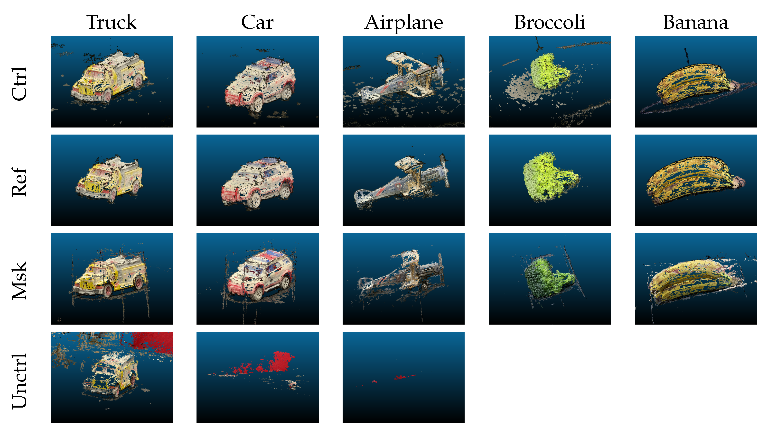
Table 6 shows the same evaluation criteria for the same objects using Pix4d SfM software. It is safe to say that the masked point clouds have a better reconstruction quality compared to the raw point clouds, which confirms the observations of Agisoft. Table 6 shows a lower number of points compared to the raw point clouds and it is more relevant to the object due to background removal. Masked point clouds are also better aligned with the reference objects since they have a lower average distance and standard deviation compared to the raw point cloud. However, the quantitative approach only applies to the yellow truck and banana objects, the other objects (car, airplane, and broccoli) have significantly lower numbers of points compared to the masked point clouds and even lower than the reference objects. For example, the masked airplane scene has 160.3 K points and the reference object has 337.3 K compared to only 14.4 K points in the raw point cloud. The significant reduction of the number of points in the raw point clouds is mainly because Pix4d failed to reconstruct those target objects (car, airplane, broccoli, and banana), shown in Figure 7. Pix4d recovered mainly the background points of the car and the airplane, and the points were scattered over a large space. The average distance and standard deviation of the two objects are not available because the registration of the raw and reference point clouds failed due to the serious deformation of the raw point clouds. Moreover, Pix4d failed to recover any points for the broccoli and the banana objects because it could not find an appropriate camera calibration. It is worth noting that Pix4d tends to drop points in rich scenes. For example, the raw point cloud of the yellow truck is missing many points in front of the car, likely because of the transformation consistency between the points. In contrast, the masked imagery successfully reconstructed all objects as shown in Figure 7 and it is almost as dense as the reference point cloud (no missing points). The background removal improved transformation consistency by removing noise and inconsistent features.

Table 7 shows the RealityCapture reconstruction results. RealityCapture recorded more or an equal number of points for the masked point clouds compared to the corresponding raw point clouds except for the banana object. Furthermore, the object-to-scene ratio shows the number of points can be as much as twice the number of points in the reference object point clouds. However, the extra number of points in the masked point cloud does not imply noise points in this case because the average distance and standard deviation from the reference point clouds are significantly lower than the corresponding raw point cloud and it also falls within the same ranges as Agisoft and Pix4d. The results suggest that RealityCapture sampled significantly more points of the objects from the masked imagery. The results also imply that RealityCapture could extract more details compared to the controlled environment. RealityCapture examples presented in Figure 8 demonstrate the generation of high-quality point clouds using the masked imagery. Figure 8 shows that most of the noise is from the points recovered from the turntable surface. The noise points do not have a significant negative impact on the recovered point cloud because it follows the same motion as the object. Furthermore, the noise points occupy a small portion of the scene which implies that most of the points in the masked point cloud belong to the object. However, sampling more points was not effective in the raw scene. For example, the airplane object is highly deformed, and the airplane structure barely appears in the point cloud. Similarly, the yellow truck is also deformed and one side of it and the car has some deformation as well. However, the broccoli and banana objects are well reconstructed except for extra background points.

In addition, Figure 9 shows the visual traits of the reconstruction when multiple objects are present in the scene. The video is processed with no additional configuration to the pipeline, and it reconstructs the two vehicles and separates them into two different point clouds. However, pix4d reconstructions are deformed, more likely because the software was not able to find appropriate camera positions and orientations to recover the correct shape of the vehicles. It is more likely because of the lower frame resolution and feature ambiguity.

Table 8. Agisoft (AG), Pix4d (PX), and RealityCapture (RC) mean and standard deviation distances relative to the reference point cloud in millimeters for multi-objects scene.

	Object	Np	O2S	Mean	SD
AG	Truck	12.5K	0.09	2.20	3.78
	Car	10.3K	0.04	0.18	0.28
PX	Truck	23.5K	0.18	2.44	7.05
	Car	18.6K	0.07	14.72	16.30
RC	Truck	60.3K	0.45	0.89	2.09
	Car	61.9K	0.25	0.856328	1.93833

shows the quantitative results of the scene where the number of extracted points is significantly lower than in previous experiments. For example, the truck is only 12.5 K points using Agisoft which is 0.09% of the reference point cloud. However, RealityCapture was able to generate more points compared to Agisoft and Pix4d. However, the number of points did not affect the reconstruction quality. Most of the objects aligned correctly with their reference point cloud with minor changes to average distance and standard deviation except for the Pix4d car reconstruction which has serious deformation and consequently it has significantly higher average distance and standard deviation from the reference point cloud.

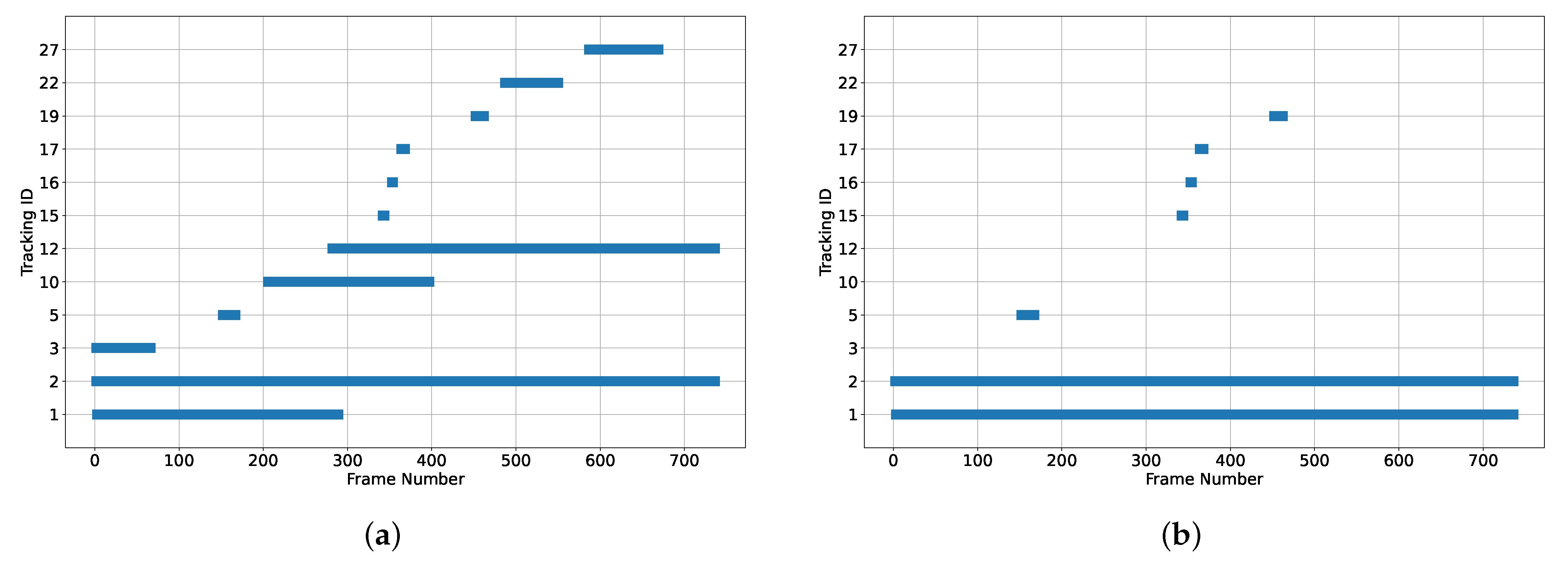
Figure 10a shows the detection and tracking profiles of the different objects in the scene; Figure 10a shows that the pipeline identifies 12 unique objects even though there are only two vehicles present in the scene. Some objects only appear for a short period of time, like objects 15 and 16. Figure 10a shows the potential issues for detection and tracking algorithms. For example, the detection network can generate multiple detections (bounding boxes) for a single object which is shown for objects 2 and 3, where they refer to the same vehicle (car object). Furthermore, the tracking algorithm may reidentify an object due to visual or motion changes (depending on similarity criterion) and lack of detection. For instance, Figure 10a shows object 1 is being tracked through about half of the video, but it then appears immediately with a different ID (12) for the rest of the video. Reidentification or track losses of objects may have a significant impact on the reconstruction quality of the objects because the loss of different views creates gaps in the resulting point clouds. So, the correction mechanism is intended to reduce the impact of track losses and object re-identification. Figure 10b shows the effect of the correction mechanism. It reduces the overall number of tracked objects from 12 to 7.

Table 9. Pipeline tracking profiles with and without the correction mechanism.

Object	Correct IDs	Merged IDs
Truck	1, 12, 17, 22	1, 12, 22
Car	2, 3, 10, 16, 27	2, 3, 10, 27
Other	5, 15, 19	5, 15, 16, 17, 19

shows the two vehicles and their corresponding IDs throughout the video and the merged IDs. The correction mechanism successfully merges the IDs of the same objects. IDs 17 and 19 are not merged because the overlap is not large enough and IDs 15 and 16 are missed due to temporal distance between frames. However, there were enough IDs to track the two vehicles correctly throughout the video, as shown in Figure 10b under the objects 1 and 2. The algorithm performance is controlled by setting the overlap and the distance between frames and the performance using a set of parameters is scene-dependent.

The results show that the pipeline is a robust mechanism where the resulting point cloud is structurally correct without deformation similar to the controlled environment, and it can be as reliable as a controlled environment for generating high-quality 3D point clouds of objects with reduced noise and artifacts. The pipeline is also independent of the SfM software, and it can improve the reconstruction quality. For example, RealityCapture sampled more points of many objects compared to the reference object point cloud which may add more fine details to the generated point cloud.

Furthermore, the experiments show that the most contributing factor in the reconstruction process is the extracted features (points) and their motion system. For example, the SfM software are able to generate a 3D point cloud from the raw imagery for all the scenes, but the yellow truck, the car, and the airplane are generally deformed and it is challenging to correct the resulting point clouds. Object deformation is common among the different software used because of their small size and rich background. The small size affected the number of features that can be extracted, and the rich background features interfered with the object motion system and reconstructed the scene incorrectly. These objects are more likely to require another scan in a controlled environment. On the other hand, the broccoli and banana objects have a rich texture that increased the number of extracted features that dominated the motion system of the scene allowing the to be reconstructed correctly in the raw scene. However, it did not prevent the additional noise in the scene from the background. The pipeline separated the different motion systems mainly the object and the background, but it is not based on clustering features based on their motion but instead based on their visual traits for both detection and tracking which elevated the need for camera information such as the focal length and radial distortion. It is important to note that blocking features such as using black background is as equally important as the extracted reconstruction features where blocking features prevents the interference between the different motion systems in the scene. It is also notable that the pipeline is scalable where it can track multiple objects at the same time and separate them from the scene. The pipeline works by removing interfering features from the scene and preserving the target region for reconstruction.

Table 10. Automatic camera calibration for the truck in the controlled environment using Agisoft, Pix4d, and RealityCapture, respectively.

F [mm]	F [pix]	Cx	Cy	K1	K2	K3	P1	P2
NA	3 × 10${}^3$	−2 × 10${}^{-1}$	−2 × 10${}^2$	−7 × 10${}^{-3}$	4 × 10${}^{-2}$	−7 × 10${}^{-2}$	−3 × 10${}^{-4}$	3 × 10${}^{-4}$
20.0	3 × 10${}^3$	2 × 10${}^3$	1 × 10${}^3$	−2 × 10${}^{-2}$	−2 × 10${}^{-2}$	1 × 10${}^{-1}$	0	0
32.0	NA	2 × 10${}^{-3}$	−4 × 10${}^{-3}$	−1 × 10${}^{-2}$	−1 × 10${}^{-1}$	5 × 10${}^{-1}$	0	0

shows the estimated camera parameters in the controlled environment for Agisoft, Pix4d, and RealityCapture, respectively. F[mm] is the estimated focal length in millimeters and F[pix] is the estimated focal length in pixels. C_x and C_y are the calibrated principal points offsets measured in pixels while the Ks and Ps are the radial and tangential distortion coefficients. The three software systems each give different camera calibration information using the same imagery of the same object. For instance, the Agisoft estimated negative values for the principal points offsets while Pix4d estimated them near the image center and RealityCapture estimated the principal points offsets is roughly 0, 0 of the image coordinates. Furthermore, the three estimated camera parameters are different from the calibrated one in Table 1. In addition to camera intrinsic parameters, the SfM software estimates the extrinsic parameters of the camera position and orientation. 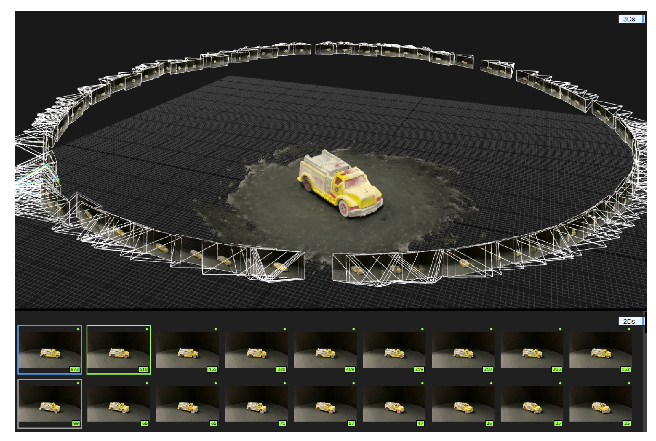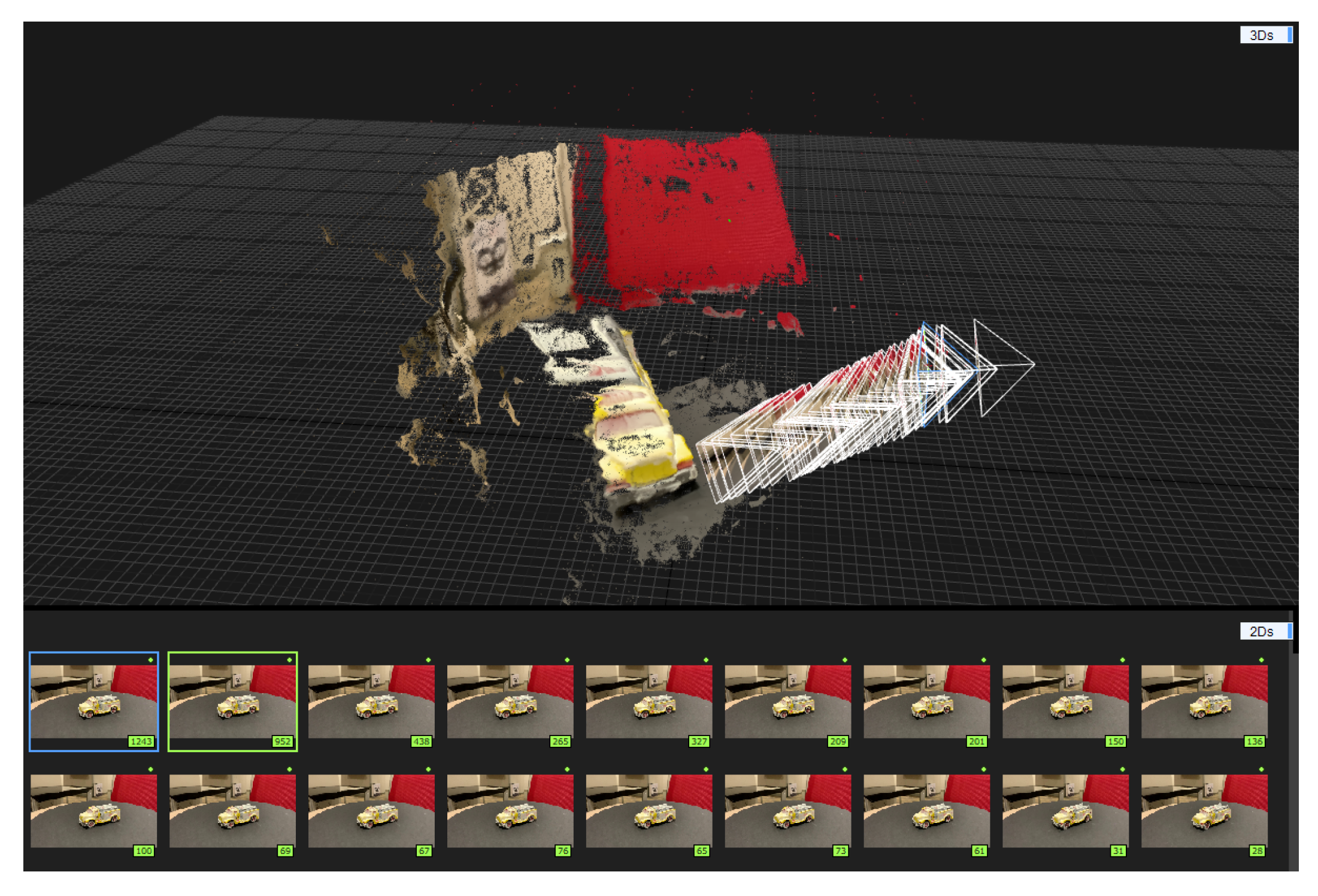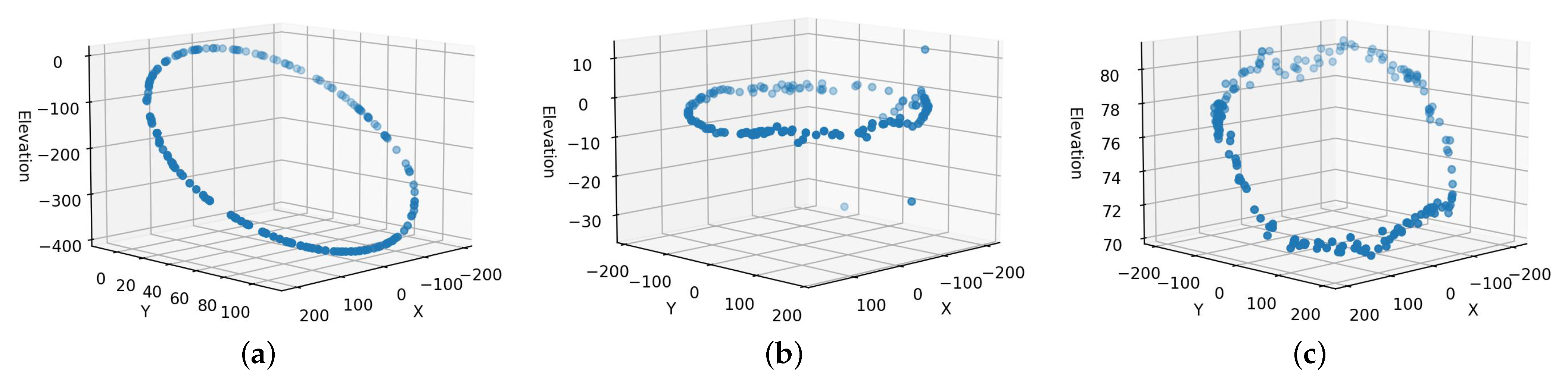Figure 11 shows the camera positions for the same experiments (the controlled environment reconstruction of the truck using Agisoft, Pix4d, and RealityCapture, after applying the same scaling factor for the same scenes in the controlled environment. The exact camera positions are not necessarily correct but the relative positions or the circular shape of the cameras are more likely to conform to the turntable movements. For example, Figure 11b shows almost a perfect circle of the camera positions around the object generated by Pix4d that is similar to the turntable’s actual setup. On the other hand, the Agisoft and RealityCapture camera positions shown in Figure 11a,c are elliptical which may introduce a shape deformation. Furthermore, the positions in Figure 11a,c show that the turntable setup is tilted. Moreover, Figure 11 suggests that the camera is rotating around the objects, but it is, in fact, stationary. These results show that accurate camera calibration is actually not necessary to reconstruct the scenes.

Furthermore, it is worth noting that the exact intrinsic and extrinsic are more likely to impact the scale of the object than the reconstruction quality. In other words, the lack of intrinsic and extrinsic camera information does not have a significant impact on the reconstruction quality (object’s shape) if it has strong distinctive features to estimate the relative camera positions and their orientation correctly. The intrinsic and extrinsic configurations that are automatically computed show the power and flexibility of the SfM to find a camera configuration to reconstruct the correct object structure even though the calibrations are highly variable. As for the scale or the accurate measurements, it can be mitigated using our scale technique to acquire measurements from the point cloud.

5. Discussion

SfM is a well-defined, powerful technique that is used to generate a 3D structure of an object or a scene. SfM software systems are employed in a wide range of applications such as agriculture and heritage preservation. However, the previous experiments demonstrate the limits of the SfM software system when processing a dynamic scene. Even with only two motion systems (the object and the rich background), the different SfM software systems are not able to generate a correct 3D point cloud. The SfM software generally needs a blank background to improve the reconstruction of the target object. The issue is magnified as the number of objects with different motions increases, making it challenging to recover usable 3D point clouds.

This research introduces a practical detection and tracking pipeline based on deep learning technology to find the object in a scene regardless of the complexity of the environment. The pipeline clusters objects based on their semantic and motion traits. The semantic features are resilient to occlusion, motion blur, or missing camera calibration information. In addition, the pipeline places a black background to obscure the environment. In other words, the framework automates the process of manual placement of a solid background that is common in a turntable setup. The framework converts a dynamic scene into multiple scenes that appear stationary and sends those to a standard reconstruction pipeline. Our pipeline also corrects common issues for the detection and tracking algorithms by merging IDs with maximum overlap. However, the technique requires an existing detection and tracking functionality and it is also limited to short track losses (within a few frames). Otherwise, it may merge incorrect objects. The pipeline is an optional noninvasive preprocessing step that augments existing software to turntable scenes without the need for additional manual setup.

Furthermore, the removal of the background before the reconstruction process would eliminate ambiguous or inconsistent features resulting from the background or the motion of the object. The framework generalizes scene reconstruction regardless of object or camera rotation which makes the pipeline valuable for stationary scenes as well. For example, scanning a real-sized car or a boat probably would need a special turntable; however, with our pipeline, capturing a video using a moving camera with a stationary object would fit directly in the standard process. Nevertheless, incorporating an artificial background to isolate the target object would improve the quality of the resulting scene, especially if there are moving objects during the scene capture. However, the proposed preprocessing step is limited to objects defined by the detection network, which can be mitigated by switching to a different detection network or retraining.

The multi-object scene results show that the pipeline can be used to segment a scene into different point clouds. Even though there are several techniques to semantically annotate or classify points in a point cloud, the projection methods are post-processing techniques that are used to semantically identify points in a point cloud. The projection methods work by taking various 2D snapshots of the point cloud from different angles, and the resulting 2D images are passed through a segmentation network to semantically classify each pixel and then project them back to a point cloud such as Snapnet [55] or Snapnet-r [56]. However, the projection methods require a point cloud in the first place which might not be feasible for a dynamic scene. On the other hand, the pipeline helps to generate 3D point clouds that are semantically valid. For example, the masked point clouds can be labeled according to their classes generated by the detection network without any further processing.

The experiments show the pipeline improves the generation quality of the 3D point clouds. However, there is no guarantee the generated point cloud would have the correct scale because there is no camera or scale information for the scene. In addition, if the scene contains multiple objects, it is not guaranteed that the different objects will have the same scale. In other words, the 3D point cloud of an object in an arbitrary video is more likely to be structurally correct but the 3D point cloud may need additional scaling. However, the manual technique can be used to scale the object correctly.

Furthermore, we did not necessarily have accurate camera parameters, as the SfM software systems can find suitable camera configurations that fit the correct structure which can be inconsistent with the actual camera or object motion, but at the cost of incorrect scale. The SfM software, in this case, relies mostly on the extracted features. In addition, our pipeline alleviates feature inconsistency because even with high SfM flexibility, the software systems are unable to handle multiple motions or dynamic scenes. Furthermore, the pipeline can be generalized to address other use cases. For example, surveying or scanning a house or a building where cars and people are moving in the scene would degrade reconstruction quality, but our pipeline can target the inconsistent features and remove them from the scene with featureless regions such as cars and people increasing quality and the likelihood of generating a point cloud.

6. Conclusions

The growing economic value of 3D modeling and related technologies is not only because of the growth of the video game industry but also because of the new advancements in virtual and augmented reality platforms, heritage preservation, and scientific applications where high quality and precision are essential traits of the 3D models. Close-range photogrammetry is a reliable method to obtain fine detailed 3D point clouds. However, it requires a rigorous setup for image collection to enhance the quality of point clouds produced by the SfM software. Even though SfM software systems are powerful tools, they cannot tolerate dynamic scenes and can only achieve high-quality reconstruction by isolating the target object from its surroundings by using a featureless background and capturing the different views of the object at close-range. In this work, we introduced an independent preprocessing deep learning-based detection and tracking pipeline for close-range SfM tasks that expand the use of visual traits for both detection and tracking separated from point-level features and camera calibration or information. The pipeline factors out the different objects in the scene into isolated subscenes that are semantically consistent. Each object is similar to close-range photogrammetry with a controlled setup that can produce high-quality 3D point clouds that would not be constructed otherwise. Furthermore, the successful reconstruction of monocular uncalibrated cameras adds value to many existing videos that can now be used to extract 3D point clouds.

References

1. Wang, Q.; Tan, Y.; Mei, Z. Computational methods of acquisition and processing of 3D point cloud data for construction applications. Arch. Comput. Methods Eng. 2020, 27, 479–499. [Google Scholar] [CrossRef]
2. Saovana, N.; Yabuki, N.; Fukuda, T. Development of an unwanted-feature removal system for Structure from Motion of repetitive infrastructure piers using deep learning. Adv. Eng. Inform. 2020, 46, 101169. [Google Scholar] [CrossRef]
3. James, D.W.; Belblidia, F.; Eckermann, J.E.; Sienz, J. An innovative photogrammetry color segmentation based technique as an alternative approach to 3D scanning for reverse engineering design. Comput.-Aided Des. Appl. 2017, 14, 1–16. [Google Scholar] [CrossRef] [Green Version]
4. Obradović, M.; Vasiljević, I.; Đurić, I.; Kićanović, J.; Stojaković, V.; Obradović, R. Virtual Reality Models Based on Photogrammetric Surveys—A Case Study of the Iconostasis of the Serbian Orthodox Cathedral Church of Saint Nicholas in Sremski Karlovci (Serbia). Appl. Sci. 2020, 10, 2743. [Google Scholar] [CrossRef]
5. Tadeja, S.K.; Lu, Y.; Rydlewicz, M.; Rydlewicz, W.; Bubas, T.; Kristensson, P.O. Exploring gestural input for engineering surveys of real-life structures in virtual reality using photogrammetric 3D models. Multimed. Tools Appl. 2021, 80, 31039–31058. [Google Scholar] [CrossRef]
6. Poux, F.; Neuville, R.; Hallot, P.; Billen, R. Smart point cloud: Definition and remaining challenges. ISPRS Ann. Photogramm. Remote Sens. Spat. Inf. Sci. 2016, 4, 119–127. [Google Scholar] [CrossRef] [Green Version]
7. Fernandes, D.; Silva, A.; Névoa, R.; Simões, C.; Gonzalez, D.; Guevara, M.; Novais, P.; Monteiro, J.; Melo-Pinto, P. Point-cloud based 3D object detection and classification methods for self-driving applications: A survey and taxonomy. Inf. Fusion 2021, 68, 161–191. [Google Scholar] [CrossRef]
8. Ahmed, H.O.; Belhi, A.; Alfaqheri, T.; Bouras, A.; Sadka, A.H.; Foufou, S. A Cost-Effective 3D Acquisition and Visualization Framework for Cultural Heritage. In Proceedings of the Fifth International Congress on Information and Communication Technology, London, UK, 23–24 April 2021; Springer: Berlin/Heidelberg, Germany, 2021; pp. 495–503. [Google Scholar]
9. Sapirstein, P. A high-precision photogrammetric recording system for small artifacts. J. Cult. Herit. 2018, 31, 33–45. [Google Scholar] [CrossRef]
10. Kochi, N.; Isobe, S.; Hayashi, A.; Kodama, K.; Tanabata, T. Introduction of All-Around 3D Modeling Methods for Investigation of Plants. Int. J. Autom. Technol. 2021, 15, 301–312. [Google Scholar] [CrossRef]
11. Porter, S.T.; Roussel, M.; Soressi, M. A simple photogrammetry rig for the reliable creation of 3D artifact models in the field: Lithic examples from the Early Upper Paleolithic sequence of Les Cottés (France). Adv. Archaeol. Pract. 2016, 4, 71–86. [Google Scholar] [CrossRef]
12. Schonberger, J.L.; Frahm, J.M. Structure-from-motion revisited. In Proceedings of the IEEE Conference on Computer Vision and Pattern Recognition, Las Vegas, NV, USA, 27–30 June 2016; pp. 4104–4113. [Google Scholar]
13. Bianco, S.; Ciocca, G.; Marelli, D. Evaluating the performance of structure from motion pipelines. J. Imaging 2018, 4, 98. [Google Scholar] [CrossRef] [Green Version]
14. Li, P.; Qin, T. Stereo vision-based semantic 3d object and ego-motion tracking for autonomous driving. In Proceedings of the European Conference on Computer Vision (ECCV), Munich, Germany, 8–14 September 2018; pp. 646–661. [Google Scholar]
15. Saputra, M.R.U.; Markham, A.; Trigoni, N. Visual SLAM and structure from motion in dynamic environments: A survey. ACM Comput. Surv. CSUR 2018, 51, 1–36. [Google Scholar] [CrossRef]
16. Aqel, M.O.; Marhaban, M.H.; Saripan, M.I.; Ismail, N.B. Review of visual odometry: Types, approaches, challenges, and applications. SpringerPlus 2016, 5, 1–26. [Google Scholar] [CrossRef] [PubMed] [Green Version]
17. Tang, C.; Wang, O.; Tan, P. Gslam: Initialization-robust monocular visual slam via global structure-from-motion. In Proceedings of the 2017 International Conference on 3D Vision (3DV), Qingdao, China, 10–12 October 2017; IEEE: Piscataway, NJ, USA, 2017; pp. 155–164. [Google Scholar]
18. Fischler, M.A.; Bolles, R.C. Random sample consensus: A paradigm for model fitting with applications to image analysis and automated cartography. Commun. ACM 1981, 24, 381–395. [Google Scholar] [CrossRef]
19. Bescos, B.; Fácil, J.M.; Civera, J.; Neira, J. DynaSLAM: Tracking, mapping, and inpainting in dynamic scenes. IEEE Robot. Autom. Lett. 2018, 3, 4076–4083. [Google Scholar] [CrossRef] [Green Version]
20. Mur-Artal, R.; Tardós, J.D. Orb-slam2: An open-source slam system for monocular, stereo, and rgb-d cameras. IEEE Trans. Robot. 2017, 33, 1255–1262. [Google Scholar] [CrossRef] [Green Version]
21. Yu, C.; Liu, Z.; Liu, X.J.; Xie, F.; Yang, Y.; Wei, Q.; Fei, Q. DS-SLAM: A semantic visual SLAM towards dynamic environments. In Proceedings of the 2018 IEEE/RSJ International Conference on Intelligent Robots and Systems (IROS), Madrid, Spain, 1–5 October 2018; IEEE: Piscataway, NJ, USA, 2018; pp. 1168–1174. [Google Scholar]
22. Badrinarayanan, V.; Kendall, A.; Cipolla, R. Segnet: A deep convolutional encoder-decoder architecture for image segmentation. IEEE Trans. Pattern Anal. Mach. Intell. 2017, 39, 2481–2495. [Google Scholar] [CrossRef]
23. Rublee, E.; Rabaud, V.; Konolige, K.; Bradski, G. ORB: An efficient alternative to SIFT or SURF. In Proceedings of the 2011 International Conference on Computer Vision, Barcelona, Spain, 6–13 November 2011; IEEE: Piscataway, NJ, USA, 2011; pp. 2564–2571. [Google Scholar]
24. Ren, S.; He, K.; Girshick, R.; Sun, J. Faster r-cnn: Towards real-time object detection with region proposal networks. In Proceedings of the Advances in Neural Information Processing Systems, Montreal, QC, Canada, 7–12 December 2015; pp. 91–99. [Google Scholar]
25. Runz, M.; Buffier, M.; Agapito, L. Maskfusion: Real-time recognition, tracking and reconstruction of multiple moving objects. In Proceedings of the 2018 IEEE International Symposium on Mixed and Augmented Reality (ISMAR), Munich, Germany, 16–20 October 2018; IEEE: Piscataway, NJ, USA, 2018; pp. 10–20. [Google Scholar]
26. He, K.; Gkioxari, G.; Dollár, P.; Girshick, R. Mask r-cnn. In Proceedings of the IEEE International Conference on Computer Vision, Venice, Italy, 22–29 October 2017; pp. 2961–2969. [Google Scholar]
27. Xu, B.; Li, W.; Tzoumanikas, D.; Bloesch, M.; Davison, A.; Leutenegger, S. Mid-fusion: Octree-based object-level multi-instance dynamic slam. In Proceedings of the 2019 International Conference on Robotics and Automation (ICRA), Montreal, QC, Canada, 20–24 May 2019; IEEE: Piscataway, NJ, USA, 2019; pp. 5231–5237. [Google Scholar]
28. Whelan, T.; Salas-Moreno, R.; Glocker, B.; Davison, A.; Leutenegger, S. ElasticFusion: Real-time dense SLAM and light source estimation. Int. J. Robot. Res. 2016, 35, 1697–1716. [Google Scholar] [CrossRef] [Green Version]
29. Hruby, P.; Pajdla, T. Reconstructing Small 3D Objects in front of a Textured Background. arXiv 2021, arXiv:2105.11352. [Google Scholar]
30. Kundu, A.; Krishna, K.M.; Jawahar, C. Realtime multibody visual SLAM with a smoothly moving monocular camera. In Proceedings of the 2011 International Conference on Computer Vision, Barcelona, Spain, 6–13 November 2011; IEEE: Piscataway, NJ, USA, 2011; pp. 2080–2087. [Google Scholar]
31. Ranftl, R.; Vineet, V.; Chen, Q.; Koltun, V. Dense monocular depth estimation in complex dynamic scenes. In Proceedings of the IEEE Conference on Computer Vision and Pattern Recognition, Las Vegas, NV, USA, 27–30 June 2016; pp. 4058–4066. [Google Scholar]
32. Chambolle, A.; Cremers, D.; Pock, T. A convex approach to minimal partitions. SIAM J. Imaging Sci. 2012, 5, 1113–1158. [Google Scholar] [CrossRef] [Green Version]
33. Casser, V.; Pirk, S.; Mahjourian, R.; Angelova, A. Depth prediction without the sensors: Leveraging structure for unsupervised learning from monocular videos. In Proceedings of the AAAI Conference on Artificial Intelligence, Honolulu, HI, USA, 27 January–1 February 2019; Volume 33, pp. 8001–8008. [Google Scholar]
34. Casser, V.; Pirk, S.; Mahjourian, R.; Angelova, A. Unsupervised monocular depth and ego-motion learning with structure and semantics. In Proceedings of the IEEE/CVF Conference on Computer Vision and Pattern Recognition Workshops, Long Beach, CA, USA, 16–17 June 2019; pp. 381–388. [Google Scholar]
35. Ran, T.; Yuan, L.; Zhang, J.; Tang, D.; He, L. RS-SLAM: A Robust Semantic SLAM in Dynamic Environments Based on RGB-D Sensor. IEEE Sensors J. 2021, 21, 20657–20664. [Google Scholar] [CrossRef]
36. Huang, J.; Yang, S.; Zhao, Z.; Lai, Y.K.; Hu, S.M. Clusterslam: A slam backend for simultaneous rigid body clustering and motion estimation. In Proceedings of the IEEE/CVF International Conference on Computer Vision, Long Beach, CA, USA, 16–17 June 2019; pp. 5875–5884. [Google Scholar]
37. Judd, K.M.; Gammell, J.D.; Newman, P. Multimotion visual odometry (mvo): Simultaneous estimation of camera and third-party motions. In Proceedings of the 2018 IEEE/RSJ International Conference on Intelligent Robots and Systems (IROS), Madrid, Spain, 1–5 October 2018; IEEE: Piscataway, NJ, USA, 2018; pp. 3949–3956. [Google Scholar]
38. Bullinger, S.; Bodensteiner, C.; Wuttke, S.; Arens, M. Moving object reconstruction in monocular video data using boundary generation. In Proceedings of the 2016 23rd International Conference on Pattern Recognition (ICPR), Cancun, Mexico, 4–8 December 2016; IEEE: Piscataway, NJ, USA, 2016; pp. 240–246. [Google Scholar]
39. Wang, C.; Luo, B.; Zhang, Y.; Zhao, Q.; Yin, L.; Wang, W.; Su, X.; Wang, Y.; Li, C. DymSLAM: 4D Dynamic Scene Reconstruction Based on Geometrical Motion Segmentation. IEEE Robot. Autom. Lett. 2020, 6, 550–557. [Google Scholar] [CrossRef]
40. LeCun, Y.; Bengio, Y.; Hinton, G. Deep learning. Nature 2015, 521, 436–444. [Google Scholar] [CrossRef]
41. Sung, F.; Yang, Y.; Zhang, L.; Xiang, T.; Torr, P.H.; Hospedales, T.M. Learning to compare: Relation network for few-shot learning. In Proceedings of the IEEE Conference on Computer Vision and Pattern Recognition, Salt Lake City, UT, USA, 18–22 June 2018; pp. 1199–1208. [Google Scholar]
42. Liu, W.; Anguelov, D.; Erhan, D.; Szegedy, C.; Reed, S.; Fu, C.Y.; Berg, A.C. Ssd: Single shot multibox detector. In Proceedings of the European Conference on Computer Vision, Amsterdam, The Netherlands, 8–16 October 2016; Springer: Berlin/Heidelberg, Germany, 2016; pp. 21–37. [Google Scholar]
43. Redmon, J.; Divvala, S.; Girshick, R.; Farhadi, A. You only look once: Unified, real-time object detection. In Proceedings of the IEEE Conference on Computer Vision and Pattern Recognition, Las Vegas, NV, USA, 27–30 June 2016; pp. 779–788. [Google Scholar]
44. Girshick, R.; Donahue, J.; Darrell, T.; Malik, J. Rich feature hierarchies for accurate object detection and semantic segmentation. In Proceedings of the IEEE Conference on Computer Vision and Pattern Recognition, Columbus, OH, USA, 23–28 June 2014; pp. 580–587. [Google Scholar]
45. Girshick, R. Fast r-cnn. In Proceedings of the IEEE International Conference on Computer Vision, Santiago, Chile, 7–13 December 2015; pp. 1440–1448. [Google Scholar]
46. Ciaparrone, G.; Sánchez, F.L.; Tabik, S.; Troiano, L.; Tagliaferri, R.; Herrera, F. Deep learning in video multi-object tracking: A survey. Neurocomputing 2020, 381, 61–88. [Google Scholar] [CrossRef] [Green Version]
47. Bewley, A.; Ge, Z.; Ott, L.; Ramos, F.; Upcroft, B. Simple online and realtime tracking. In Proceedings of the 2016 IEEE International Conference on Image Processing (ICIP), Phoenix, AZ, USA, 25–28 September 2016; IEEE: Piscataway, NJ, USA, 2016; pp. 3464–3468. [Google Scholar]
48. Wojke, N.; Bewley, A.; Paulus, D. Simple Online and Realtime Tracking with a Deep Association Metric. In Proceedings of the 2017 IEEE International Conference on Image Processing (ICIP), Beijing, China, 17–20 September 2017; IEEE: Piscataway, NJ, USA, 2017; pp. 3645–3649. [Google Scholar] [CrossRef] [Green Version]
49. Wojke, N.; Bewley, A. Deep Cosine Metric Learning for Person Re-identification. In Proceedings of the 2018 IEEE Winter Conference on Applications of Computer Vision (WACV), Lake Tahoe, NV, USA, 12–15 March 2018; IEEE: Piscataway, NJ, USA, 2018; pp. 748–756. [Google Scholar] [CrossRef] [Green Version]
50. Kalman, R.E. A new approach to linear filtering and prediction problems. J. Basic Eng. 1960, 82, 35–45. [Google Scholar] [CrossRef] [Green Version]
51. Lin, T.Y.; Maire, M.; Belongie, S.; Hays, J.; Perona, P.; Ramanan, D.; Dollár, P.; Zitnick, C.L. Microsoft coco: Common objects in context. In Proceedings of the European Conference on Computer Vision, Zurich, Switzerland, 6–12 September 2014; Springer: Berlin/Heidelberg, Germany, 2014; pp. 740–755. [Google Scholar]
52. Zhang, Z. A flexible new technique for camera calibration. IEEE Trans. Pattern Anal. Mach. Intell. 2000, 22, 1330–1334. [Google Scholar] [CrossRef] [Green Version]
53. CloudCompare—Open Source Project. 2019. Available online: https://www.cloudcompare.org/doc/wiki/index.php?title=Introduction (accessed on 2 October 2020).
54. Cloud-to-Cloud Distance—CloudCompareWiki. Available online: https://www.cloudcompare.org/doc/wiki/index.php?title=Cloud-to-Cloud_Distance (accessed on 18 January 2022).
55. Boulch, A.; Le Saux, B.; Audebert, N. Unstructured Point Cloud Semantic Labeling Using Deep Segmentation Networks. In Proceedings of the 3DOR@ Eurographics—Eurographics Workshop on 3D Object Retrieval, Lyon, France, 23–24 April 2017; Volume 3, pp. 1–8. [Google Scholar]
56. Guerry, J.; Boulch, A.; Le Saux, B.; Moras, J.; Plyer, A.; Filliat, D. Snapnet-r: Consistent 3d multi-view semantic labeling for robotics. In Proceedings of the IEEE International Conference on Computer Vision Workshops, Venice, Italy, 22–29 October 2017; pp. 669–678. [Google Scholar]
Figure 1. Example of controlled environment reconstruction.
Remotesensing 14 03199 g001
Figure 2. Example of uncontrolled environment reconstruction.
Remotesensing 14 03199 g002
Figure 3. Incremental Structure from Motion pipeline.
Remotesensing 14 03199 g003
Figure 4. Abstract view of our Proposed pipeline.
Remotesensing 14 03199 g004
Figure 5. Reconstructed image samples from the controlled environment (Ctrl), the uncontrolled environment (Unctrl) and masked (Msk).
Remotesensing 14 03199 g005
Figure 6. Example results using Agisoft controlled environment, Ref—hand cleaned version of Ctrl, Msk—uncontrolled environment masked using our pipeline, Unctrl—uncontrolled environment.
Remotesensing 14 03199 g006
Figure 7. Example results using Pix4d for various models showing the four resulting point clouds from out experiments. Ctrl—using controlled environment, Ref—hand cleaned version of Ctrl, Msk—uncontrolled environment masked using our pipeline, Unctrl—uncontrolled environment.
Remotesensing 14 03199 g007
Figure 8. Example results using RealityCapture for various models showing the four resulting point clouds from out experiments. Ctrl—using controlled environment, Ref—hand cleaned version of Ctrl, Msk—uncontrolled environment masked using our pipeline, Unctrl—uncontrolled environment.
Remotesensing 14 03199 g008
Figure 9. Agisoft (AG), Pix4d (PX), and RealityCaptures (RC) visuals for the different point clouds.
Remotesensing 14 03199 g009
Figure 10. Gantt chart of the pipeline tracking profiles with and without using the correction mechanism showing the time span of each distinct object ID over the entire video. (a) Tracking profiles without the correction mechanism. (b) Tracking profiles using the correction mechanism which identifies and merges duplicate IDs.
Remotesensing 14 03199 g010
Figure 11. Camera positions and heights in millimeters for the truck recording in standard turntable environment using Agisoft (AG), Pix4d (PX), and RealityCapture (RC). (a) AG camera 3D positions. (b) PX camera 3D positions. (c) RC camera 3D positions.
Remotesensing 14 03199 g011