Article

Subsurface Temperature Reconstruction for the Global Ocean from 1993 to 2020 Using Satellite Observations and Deep Learning

1
Key Laboratory of Spatial Data Mining and Information Sharing of Ministry of Education, National & Local Joint Engineering Research Center of Satellite Geospatial Information Technology, Fuzhou University, Fuzhou 350108, China
2
State Key Laboratory of Marine Environmental Science, Xiamen University, Xiamen 361005, China
3
Center for Remote Sensing, College of Earth, Ocean and Environment, University of Delaware, Newark, DE 19716, USA
*
Author to whom correspondence should be addressed.
Remote Sens. 2022, 14(13), 3198; https://doi.org/10.3390/rs14133198
Submission received: 26 May 2022 / Revised: 26 June 2022 / Accepted: 30 June 2022 / Published: 3 July 2022
(This article belongs to the Section Ocean Remote Sensing)

Abstract

:
The reconstruction of the ocean’s 3D thermal structure is essential to the study of ocean interior processes and global climate change. Satellite remote sensing technology can collect large-scale, high-resolution ocean observation data, but only at the surface layer. Based on empirical statistical and artificial intelligence models, deep ocean remote sensing techniques allow us to retrieve and reconstruct the 3D ocean temperature structure by combining surface remote sensing observations with in situ float observations. This study proposed a new deep learning method, Convolutional Long Short-Term Memory (ConvLSTM) neural networks, which combines multisource remote sensing observations and Argo gridded data to reconstruct and produce a new long-time-series global ocean subsurface temperature (ST) dataset for the upper 2000 m from 1993 to 2020, which is named the Deep Ocean Remote Sensing (DORS) product. The data-driven ConvLSTM model can learn the spatiotemporal features of ocean observation data, significantly improves the model’s robustness and generalization ability, and outperforms the LighGBM model for the data reconstruction. The validation results show our DORS dataset has high accuracy with an average R2 and RMSE of 0.99/0.34 °C compared to the Argo gridded dataset, and the average R2 and NRMSE validated by the EN4-Profile dataset over the time series are 0.94/0.05 °C. Furthermore, the ST structure between DORS and Argo has good consistency in the 3D spatial morphology and distribution pattern, indicating that the DORS dataset has high quality and strong reliability, and well fills the pre-Argo data gaps. We effectively track the global ocean warming in the upper 2000 m from 1993 to 2020 based on the DORS dataset, and we further examine and understand the spatial patterns, evolution trends, and vertical characteristics of global ST changes. From 1993 to 2020, the average global ocean temperature warming trend is 0.063 °C/decade for the upper 2000 m. The 3D temperature trends revealed significant spatial heterogeneity across different ocean basins. Since 2005, the warming signal has become more significant in the subsurface and deeper ocean. From a remote sensing standpoint, the DORS product can provide new and robust data support for ocean interior process and climate change studies.

1. Introduction

The ocean acts as a heat sink and greatly modulates the Earth’s energy balance. The ocean absorbs about 90% of the excess heat trapped in the climate system [1]; the huge heat storage in the ocean causes significant ocean warming and leads to sea level rise [2]. Quantitative and accurate monitoring of the internal thermal structure of the ocean is the foundation for detecting and understanding changes in the Earth’s Energy Imbalance [3,4], as well as ocean heat sequestration and redistribution during global warming and hiatus [5,6,7]. Ocean temperature is the most direct reflection of changes in the global ocean’s internal thermal structure. Internal ocean temperature observations are sparse and inhomogeneous, which severely limits study on ocean warming and dynamic processes [8,9]. Although the Argo float observing network has achieved global ocean observations within a depth range of 0–2000 m, there are still data gaps in the pre-Argo period. The ocean’s internal dynamic processes, characterized by multiple spatiotemporal scales, are complicated [10,11]. The time series of the Argo float dataset is too short to support long-term ocean phenomena analysis. As a result, long-term reconstruction of the global ocean subsurface temperature (ST) dataset is imperative.
Satellite remote sensing technology provided large-scale and high-spatiotemporal-resolution, as well as long-time-series, ocean observation in the 1970s, which aided the development of atmospheric and marine sciences [12,13]. However, due to the physical properties of the ocean, the electromagnetic waves of satellite remote sensing cannot penetrate directly into the ocean, making direct observation of the ocean’s internal information impossible [14]. Some studies have indicated that certain physical phenomena and changes within the ocean have surface manifestations that can be detected by satellite remote sensing [15]. By developing a certain model of the relationship between satellite-based sea surface observations and float-based subsurface observations, the environmental parameters within the ocean can be accurately retrieved [16,17]. Through deep ocean remote sensing (DORS) techniques combining satellite data and Argo data, it is possible to realize the expansion of satellite observations from the surface to the subsurface as well as the time sequence from the back to the front. So far, empirical statistical methods [18,19,20,21], and artificial intelligence data-driven methods [14,17,22,23,24,25] have become the most common and popular methods for developing DORS techniques.
With the increasing number of ocean observations, the large amount of ocean data (including remote sensing and float data) is sufficient to build new data-driven methods such as deep learning models for developing DORS techniques. Nowadays, advanced artificial intelligence technology has a new impetus for the inversion and reconstruction of ocean internal parameters. In big data modeling, deep learning networks can capture more spatiotemporal features than machine learning methods [26,27]. Convolutional neural networks (CNN), which have the advantage of capturing spatial feature information, and long short-term memory (LSTM), which solves time series dependency problems, are frequently used in the fields of geoscience and remote sensing. CNN can well learn the spatial pattern and relationships of the input data, and can achieve high accuracy in the spatial distribution [28,29]. The subsurface thermohaline structure can be well predicted based on LSTM and its variants, and the accuracy is higher than methods such as random forests (RFs) [30], recurrent neural network (RNN) [31], support vector regression (SVR), and multilayer perceptron regressor (MLPR) [32]. LSTM is not only suitable for the inversion of ocean subsurface temperature but also has a good application in predicting other ocean internal parameters [33], such as the time series reconstruction of global ocean heat content for the upper 2000 m [34]. Because of ocean data’s inherent spatial nonlinearity and temporal dependence, traditional LSTM and CNN cannot fully exploit the temporal and spatial properties of ocean data. As a result, the ConvLSTM algorithm was proposed to extend LSTM [35]. The model can account for not only the time series dependence of ocean data but also the spatial characteristics of ocean data, allowing it to better capture the characteristics of temporal and spatial changes in the ocean.
The purpose of this study is to develop a new spatiotemporal deep learning model to reconstruct the time series global ocean ST dataset using the ConvLSTM algorithm by combining multisource remote sensing observations with Argo float observations. Here, a new long-time-series and global-scale DORS product based on satellite remote sensing and AI is reconstructed for tracking global ocean warming from 1993 to 2020. This new satellite-based DORS product is promising and has great potential to support the study of global ocean warming and climate change from a remote sensing perspective.

2. Study Area and Data

The ocean, as a massive heat storage reservoir, is critical to the global climate system. The study area spans 180°W–180°E and 78.375°S–77.625°N, primarily covering the Pacific, Atlantic, Indian, and Southern Oceans (Figure 1).
To reconstruct a time series model, this study combines surface remote sensing observations with Argo float observations: (1) sea surface temperature (SST), sea surface height (SSH), sea surface wind, and the sea surface wind field, which can be decomposed into northward and eastward components (USSW, VSSW); and (2) Argo gridded ocean temperature data in the upper 2000 m since 2005, including 23 standard layers. Moreover, Institute of Atmospheric Physics (IAP) gridded ocean temperature data from the Institute of Atmospheric Sciences, Chinese Academy of Sciences [6], EN4 analyses and profile ocean temperature data of the British Meteorological Service Hadley Centre [36], Ishii data provided by the Meteorological Institute of the Japan Meteorological Agency [37], and ARMOR3D ocean temperature data provided by the European Copernicus Service [18] were used in this study for accuracy validation (Table 1).

3. Methods

3.1. ConvLSTM Neural Network

LSTM, as a special recurrent neural network (RNN) structure, performs well in processing time series data with temporal correlation. However, when processing spatiotemporal data, it does not encode spatial information, resulting in excessive spatial redundancy, and the spatial data has strong local characteristics that LSTM cannot describe. The ConvLSTM model is an LSTM variant that can be used to solve spatiotemporal prediction problems. The purpose of ConvLSTM is to predict the precipitation of adjacent time nodes, which is a time series problem [35]. Because the ocean observation data used in this study have inherent spatial nonlinearity and temporal dependence, the reconstruction of the global ST structure can be thought of as a spatiotemporal prediction problem, with input and output targets and also spatiotemporal sequences. The ConvLSTM algorithm can account for not only the time series dependence of ocean data but also the spatial correlation of ocean data. Furthermore, the governing equations of oceanic dynamics, the Navier-Stokes equation, is a set of equations with nonlinear and time-dependent terms. Hence, we consider that our ConvLSTM method can better grasp these features and improve the prediction accuracy. ConvLSTM proposes a ConvLSTM unit with a convolutional structure in the input-to-state and state-to-state transitions by extending the LSTM, that is, by changing the traditional LSTM fully connected layer to a convolutional layer.

3.2. LightGBM

The light-gradient-boosting machine (LightGBM) [38], proposed by Microsoft Research Asia, is a gradient-boosting framework and an improved algorithm for the gradient-boosted decision tree (GBDT) model. LightGBM solves the shortcomings of the traditional boosting algorithm in scalability and running speed. The model supports parallel learning, which can greatly reduce the training time and computational cost. At present, LightGBM has been effectively applied in the field of remote sensing. LightGBM is superior to other classic machine learning methods [39]. Therefore, this study employed LightGBM as a comparison model.

3.3. Experimental Design

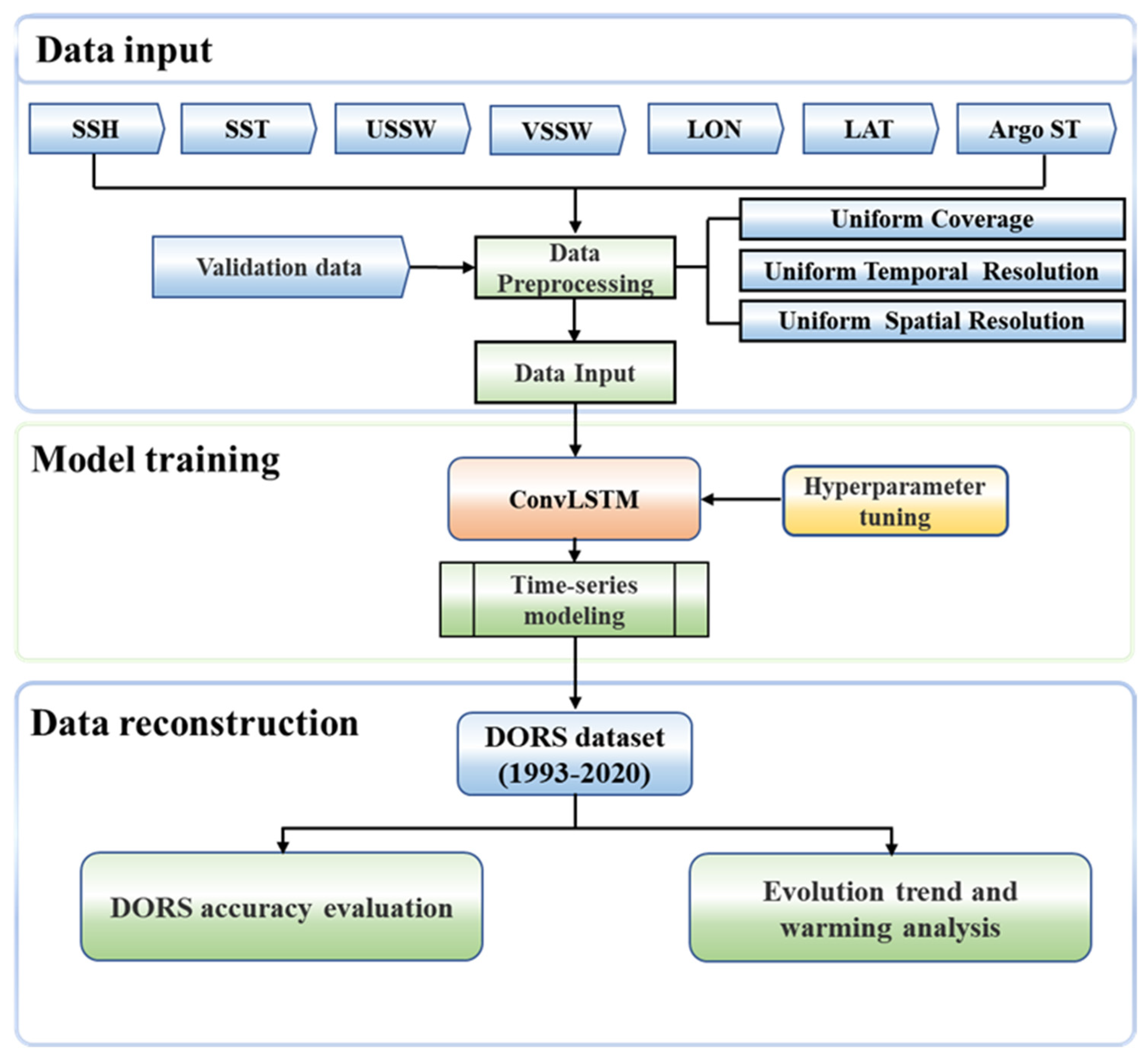
Figure 2 depicts the overall experiment technical flowchart, which is divided into three steps: model setup, time series reconstruction, and accuracy evaluation. A training set of surface remote sensing observations from 2010 to 2015 and Argo float observation is used in this study: longitude, latitude, SSH, SST, USSW, VSSW, and the training label is Argo gridded data. The reconstruction accuracy of the model is quantitatively evaluated in this study using R2, RMSE, and normalized root-mean-square error (NRMSE) indicators.
Based on the ConvLSTM model, this study reconstructs an end-to-end trainable model to deal with the global ST structure reconstruction problem. The data acceptance form of the ConvLSTM network is a 4D tensor of (time step, image height, image width, image channel). In the data component stage, the training set needs to be organized as a 5D tensor (image batch, time step, image height, image width, image channel). The vital parameters of the model that are tuned to the optimal ones by the grid search strategy are shown in Table 2. The activation function used here is Elu, and we set the optimizer to RMSprop and the maximum number of epochs to 4000. The ConvLSTM network structure has 1 input layer, 11 hidden layers, and 1 output layer. The ConvLSTM2D layer is chosen by the hidden layer, along with the BatchNormalization layer and the Dropout layer, and the ConvLSTM3D layer is chosen by the output layer. For the LightGBM model, there are three important hyperparameters: the number of leaf nodes, the learning rate, and the number of iterations. We set them as 30, 0.5, and 3000, respectively, by grid-search hyperparameter tuning.

4. Results and Discussion

4.1. Accuracy Comparison between the ConvLSTM and LightGBM Models

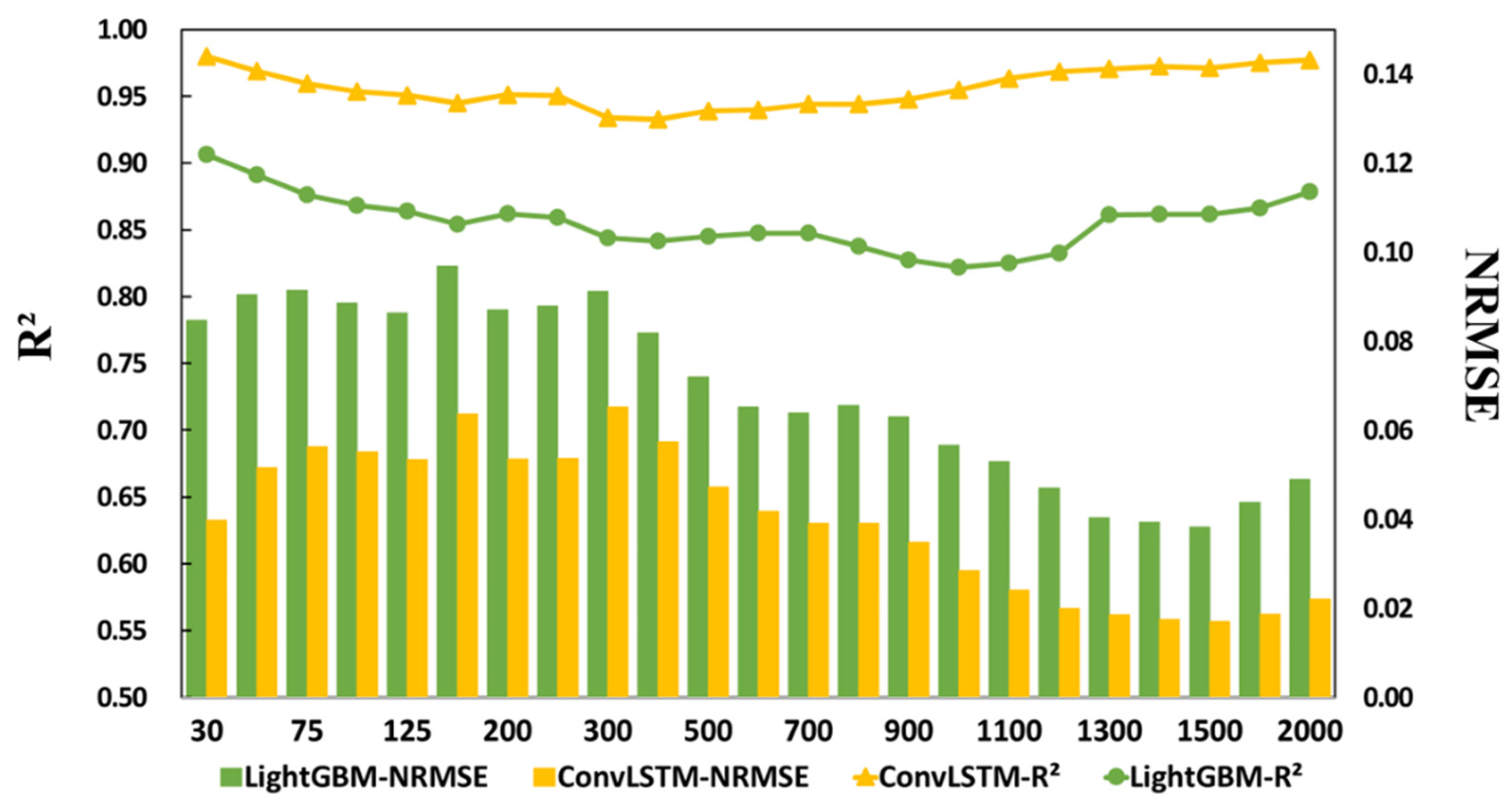
Here, in order to validate the advantages of the ConvLSTM model, we employed the advanced LightGBM method as a comparison algorithm. We established time series ConvLSTM and LightGBM models to estimate ST at different depth levels in January 2016 and evaluated the accuracy using the EN4-Profile dataset by R2 and NRMSE indicators (NRMSE is the RMSE divided by the range of the EN4-Profile ST values at the current depth level). The R2 of the ConvLSTM were higher than the LightGBM and the NRMSE were lower than the LightGBM at different depth levels (Figure 3), which suggests that the ConvLSTM model has better performance and higher accuracy than the LightGBM model, regardless of the depth. Overall, the ConvLSTM model outperformed the LightGBM model in subsurface temperature estimation because the deep-neural-network-based method has an advantage in learning the spatiotemporal features of the ocean data.

4.2. DORS Dataset and Accuracy Evaluation

Here, a new long-time-series global ocean ST dataset (DORS) was reconstructed using the aforementioned ConvLSTM model by combining multisource remote sensing observations with Argo float observations. The DORS dataset contains 23 depth layers (from 30 m to 2000 m depth) and is a monthly dataset from 1993 to 2020 with a spatial resolution of 1° × 1°, which has been shared and can be freely accessed (http://www.doi.org/10.57760/sciencedb.01918, accessed on 1 April 2022).

4.2.1. Time Series Accuracy Evaluation

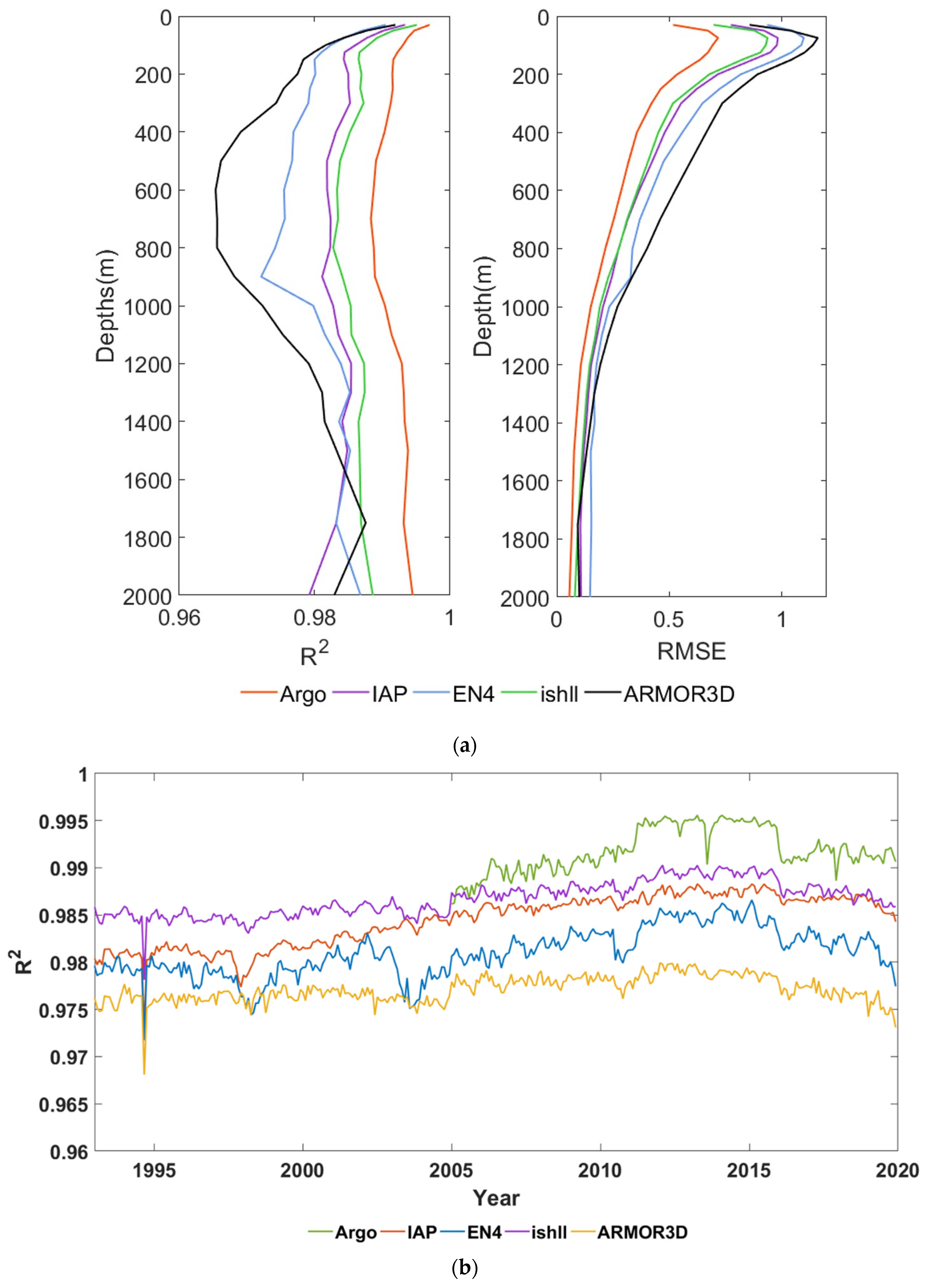
The DORS dataset and the Argo/IAP/EN4/Ishii/ARMOR3D dataset are used for consistency comparison and quality validation based on the evaluation indicators R2 and RMSE (Figure 4). The R2 of the DORS dataset and the validation dataset decreased gradually with increasing depth at the 0–600 m layers and decreased rapidly at 100–500 m (Figure 4a). The disturbance of seawater in the mixed layer and thermocline may render internal phenomena of the ocean insignificant in the surface layer, resulting in a decrease in the model reconstruction accuracy. At 800–1300 m, the R2 showed an upward trend again, and the correlation trend with the IAP and ARMOR3D datasets at 1800–2000 m was different from the other datasets and showed a downward trend with the increase in depth. In general, the R2 of the DORS and Argo/IAP/Ishii datasets remained above 0.98 at 0–2000 m, and the overall fluctuation was small, whereas the R2 of the dataset and EN4 /ARMOR3D fluctuated more at the 100–800 m layers, but it remained above 0.96. When compared to the validation datasets, the DORS had similar changes in the multiyear average RMSE at different depths. Except for the rising trend of the RMSE in the mixed layer (0–100 m), the RMSEs of the other layers all showed a downward trend with the increase in depth. Because the temperature of the ocean gradually decreases with depth, the range and variance of ST are small, so the RMSE is kept in a low range.
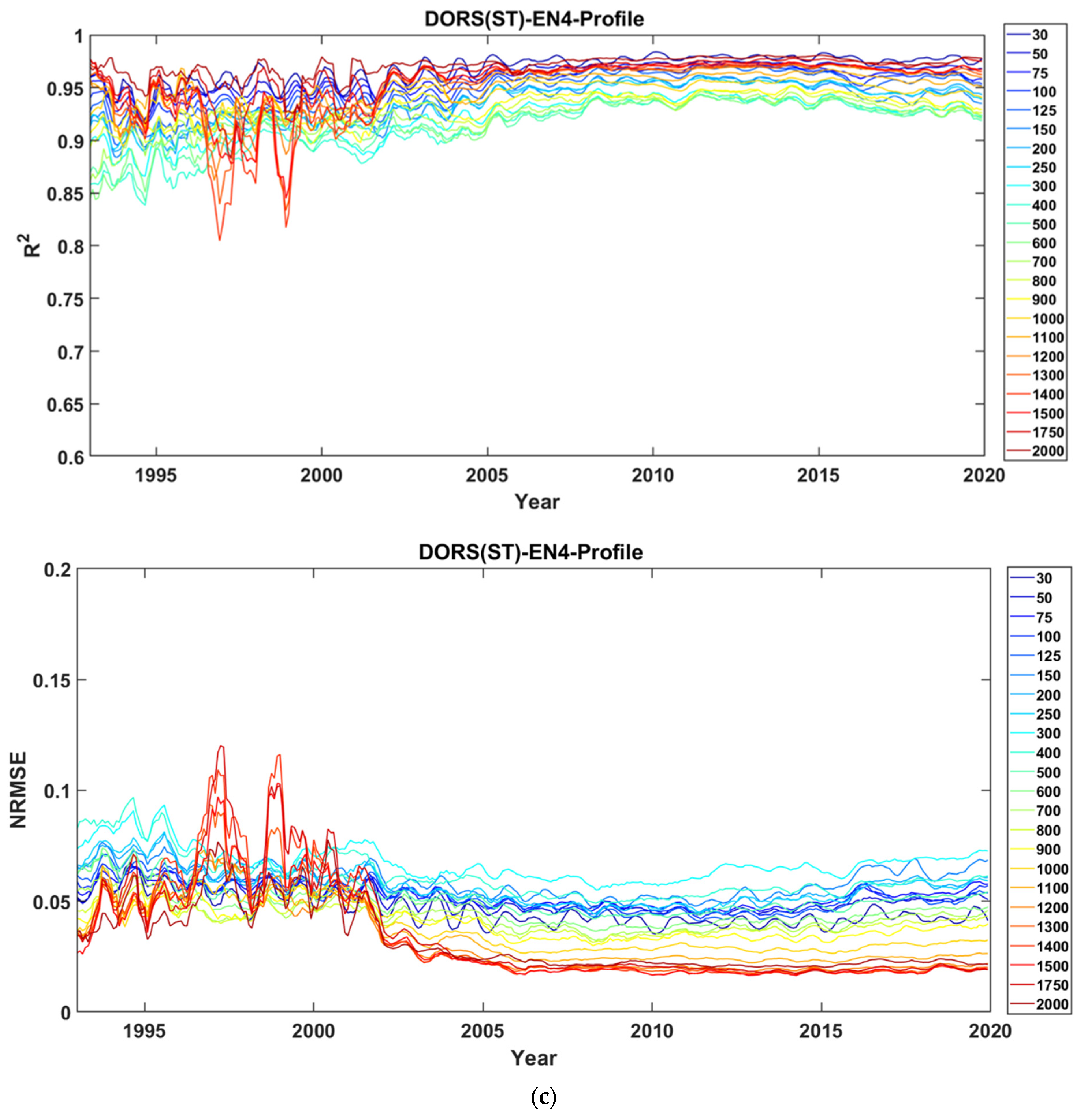
The average R2 and RMSE of DORS relative to Argo over the time series were 0.99/0.34 °C, respectively (Figure 4b). The average R2 and RMSE with IAP were 0.98/0.46 °C. The average R2 and RMSE with EN4 were 0.98/0.53 °C. The average R2 and RMSE with Ishii were 0.99/0.44 °C. The average R2 and RMSE with ARMOR3D were 0.98/0.57 °C. Overall, DORS had the highest R2 with Argo and the lowest with ARMOR3D. Our DORS dataset, reconstructed from satellite observations and deep learning, has high consistency with the various gridded datasets (with high R2 ranging from 0.97 to 0.99), and the discrepancies among the different datasets are really low and indistinctive. The DORS also has high prediction accuracy, validated by the EN4-Profile dataset over the whole time series from 1993 to 2020. The average R2 and NRMSE validated by EN4-Profile dataset over the time series were 0.94/0.05 °C, respectively (Figure 4c). Although there are some fluctuations in the accuracy indicators for the prediction at deep layer, the overall accuracy is relatively high and stable over different years and different depth levels. The R2 is almost above 0.90, and the NRMSE ranges from 0.02 to 0.08 °C generally. Overall, the DORS dataset has high accuracy and high consistency with each validation dataset, which shows great potential in ocean process and climate change applications.

4.2.2. Spatial Distribution Validation

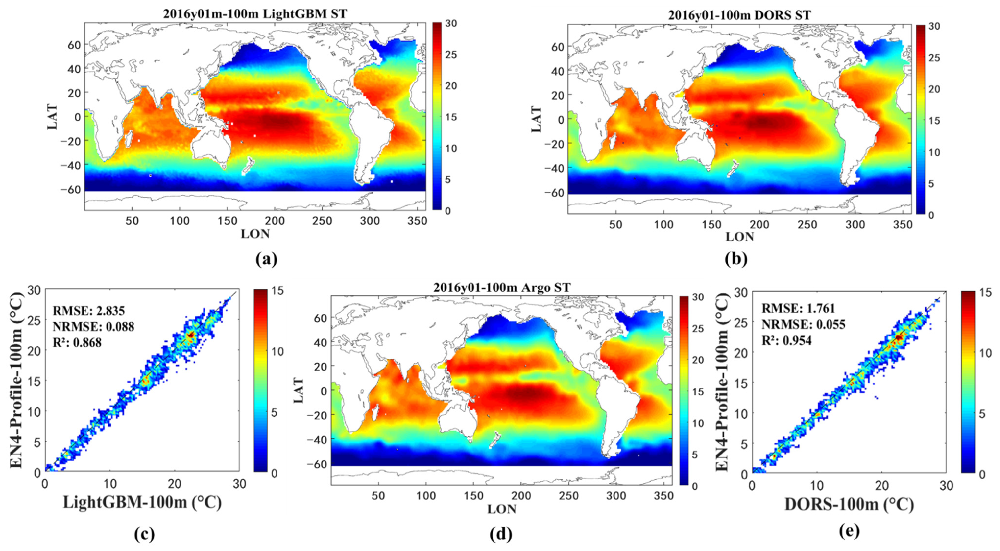
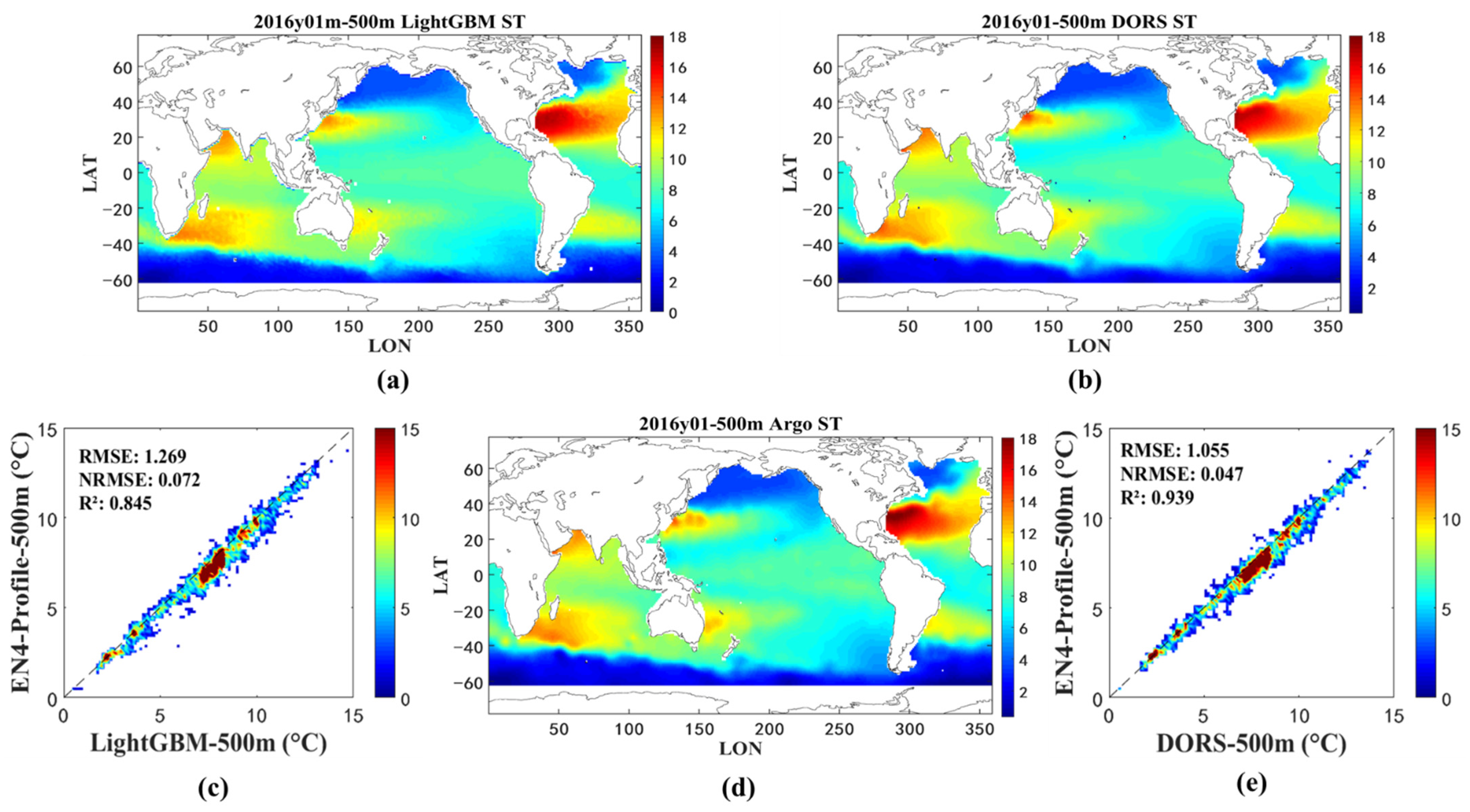
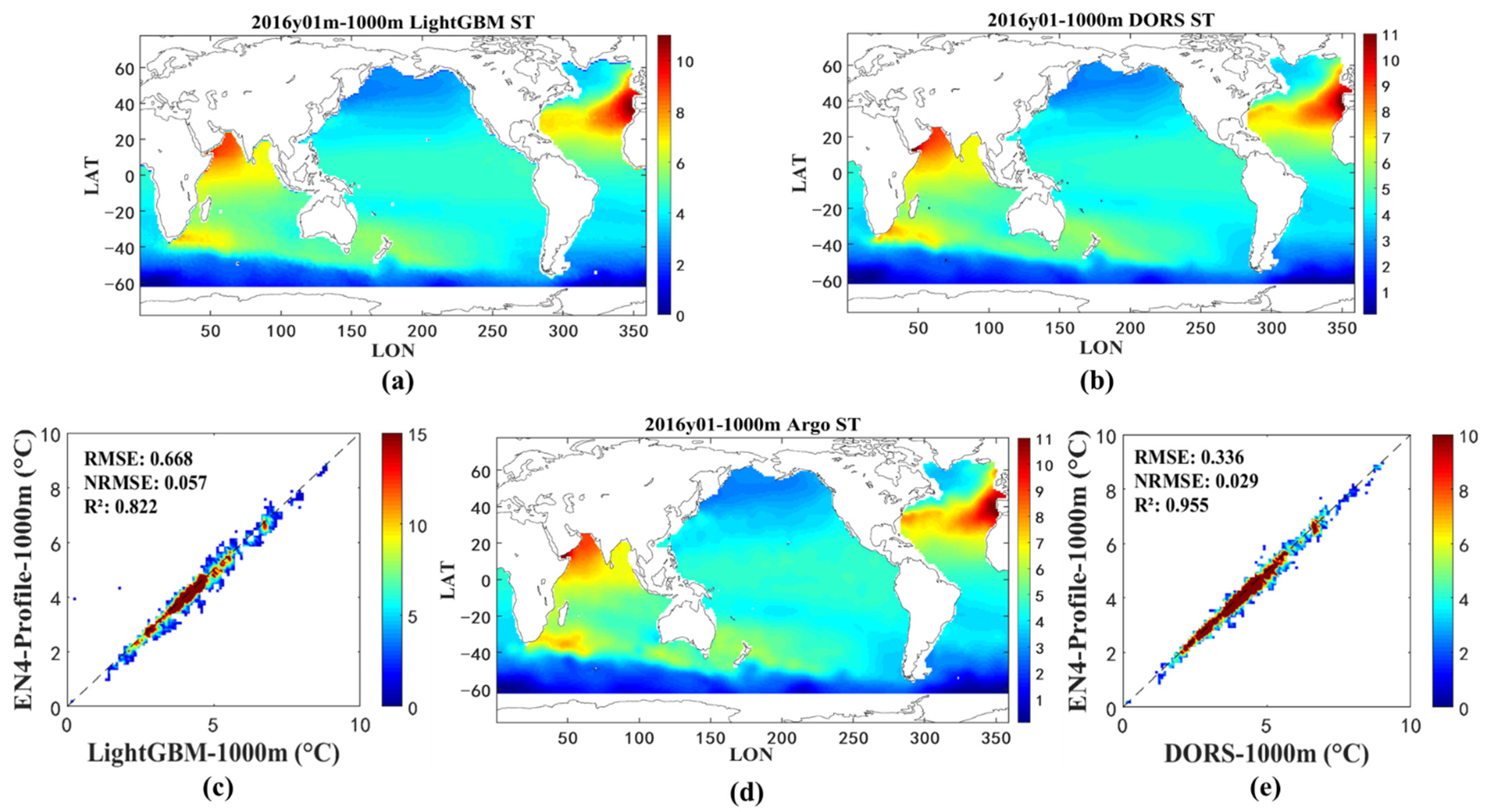
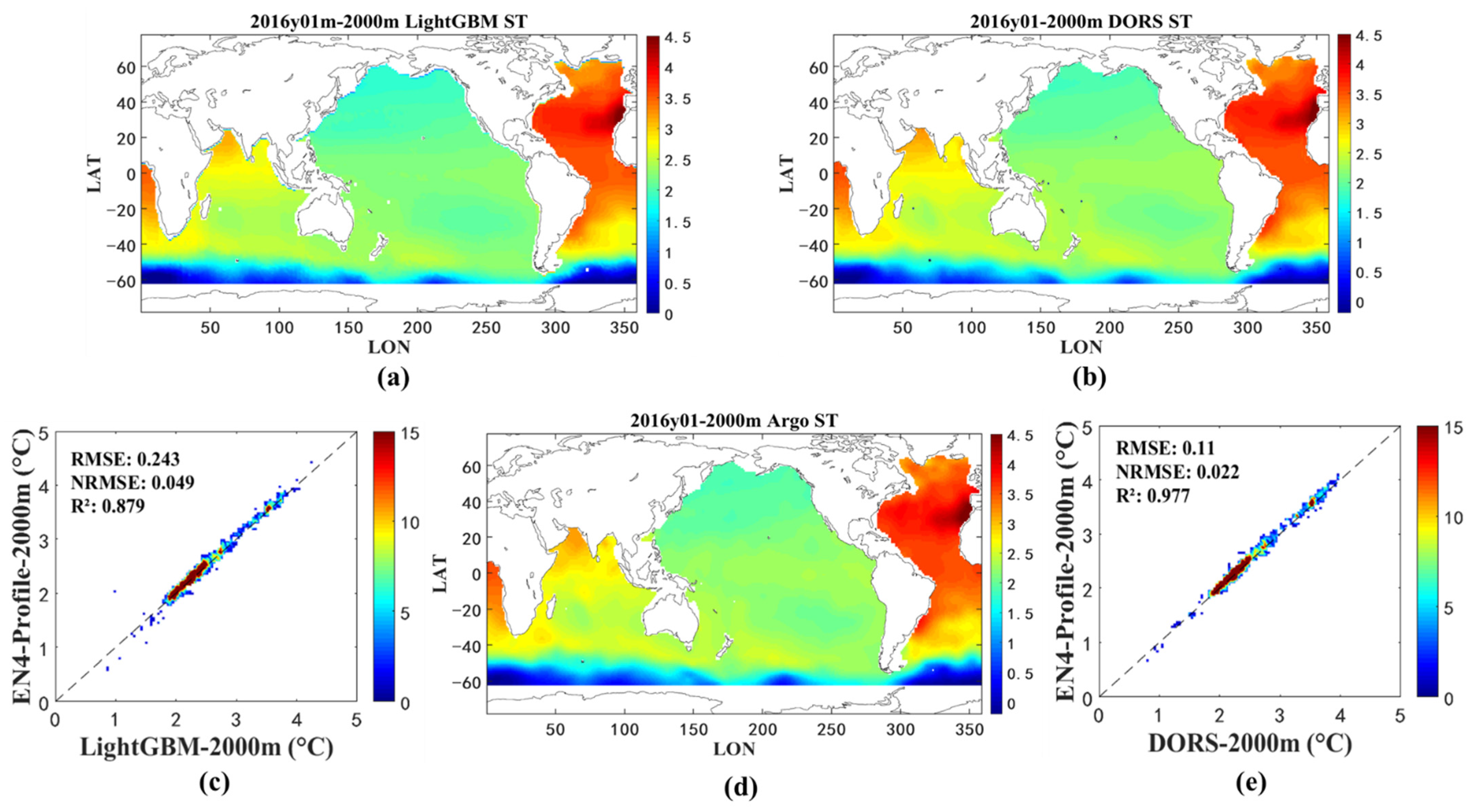
The spatial distribution differences in our reconstructed datasets were compared to the validation datasets at the same time (January 2016) and layer. Figure 5, Figure 6, Figure 7 and Figure 8 depict the spatial distribution of the reconstructed subsurface temperature for different layers (100 m, 500 m, 1000 m, and 2000 m) based on the ConvLSTM model, LightGBM model, and Argo dataset, and the intensity scatter plots between the EN4-Profile ST and reconstructed ST. It is clear that the spatial patterns of subsurface temperature between DORS and Argo are quite similar, while there are some deviations in some regions between LightGBM and Argo at different depth levels. The scatter density plot shows that DORS is highly correlated with EN4-Profile, regardless of depth levels. The R2 of DORS is higher than that of LightGBM, while the RMSE of DORS is lower at different depth levels.
A wide range of high-temperature zones can be observed at the 100 m depth level, ranging from 30°S to 30°N (Figure 5a,d). Meanwhile, there are some low-temperature zones from 40°S to 60°S and from 40°N to 60°N. The high-value area of the global ocean temperature shrinks at the 500 m depth level. The North Atlantic Ocean has the highest temperature (Figure 6a,d). The spatial distribution at 1000 m is similar to that at 500 m (Figure 7a,d). The Atlantic Ocean temperature is warmer than the other ocean basins at 2000 m (Figure 8a,d). The spatial distributions of the DORS and Argo dataset at all layers are generally consistent, and there is no abrupt excursion. This demonstrates that the ConvLSTM performance is robust and effective, and the spatial distribution characteristics of global subsurface temperature are well learned. The ConvLSTM model outperforms the LightGBM model in both consistency and accuracy, implying that the reconstruction quality of the DORS dataset is good.

4.2.3. Vertical Distribution Validation

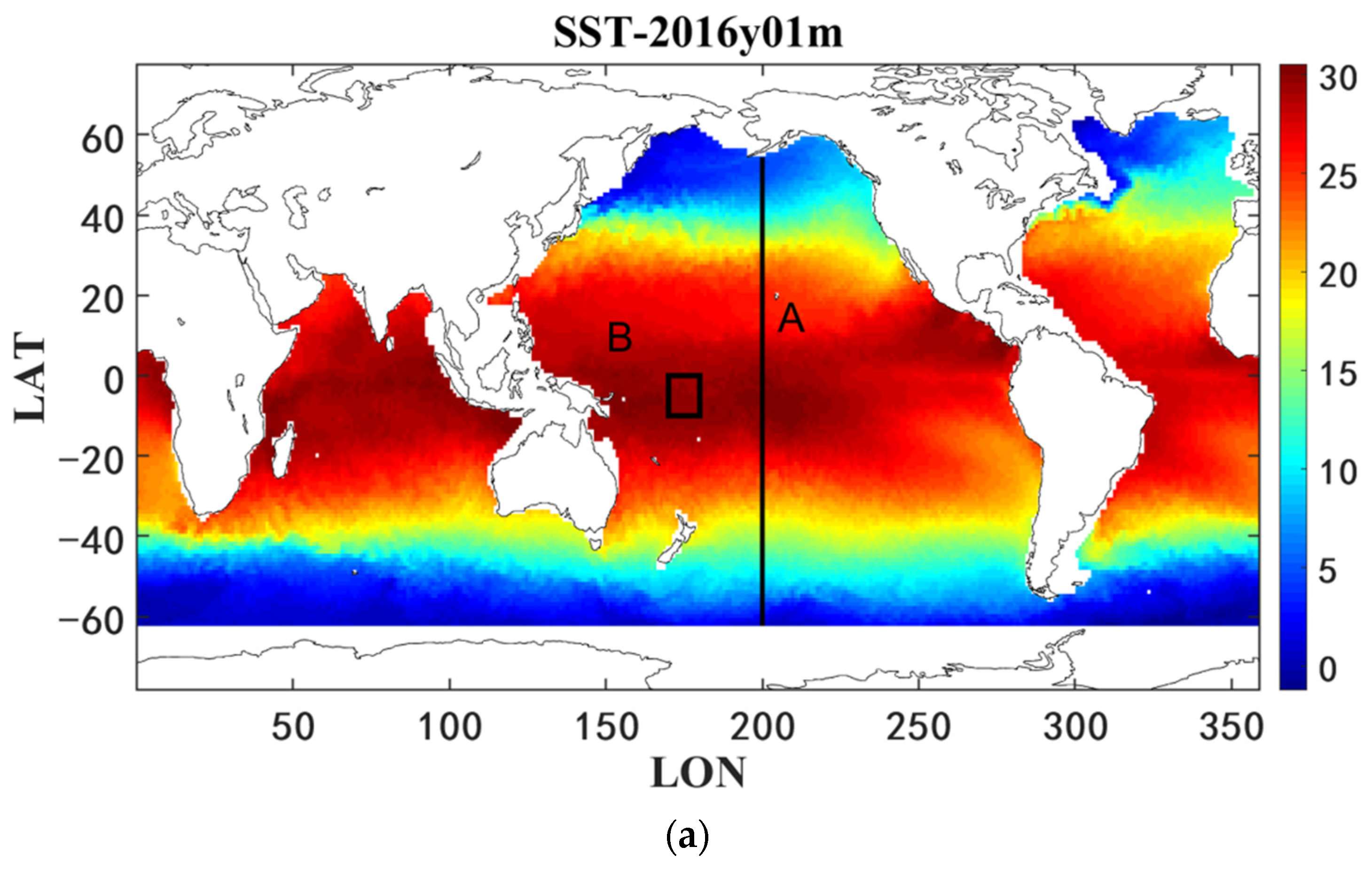
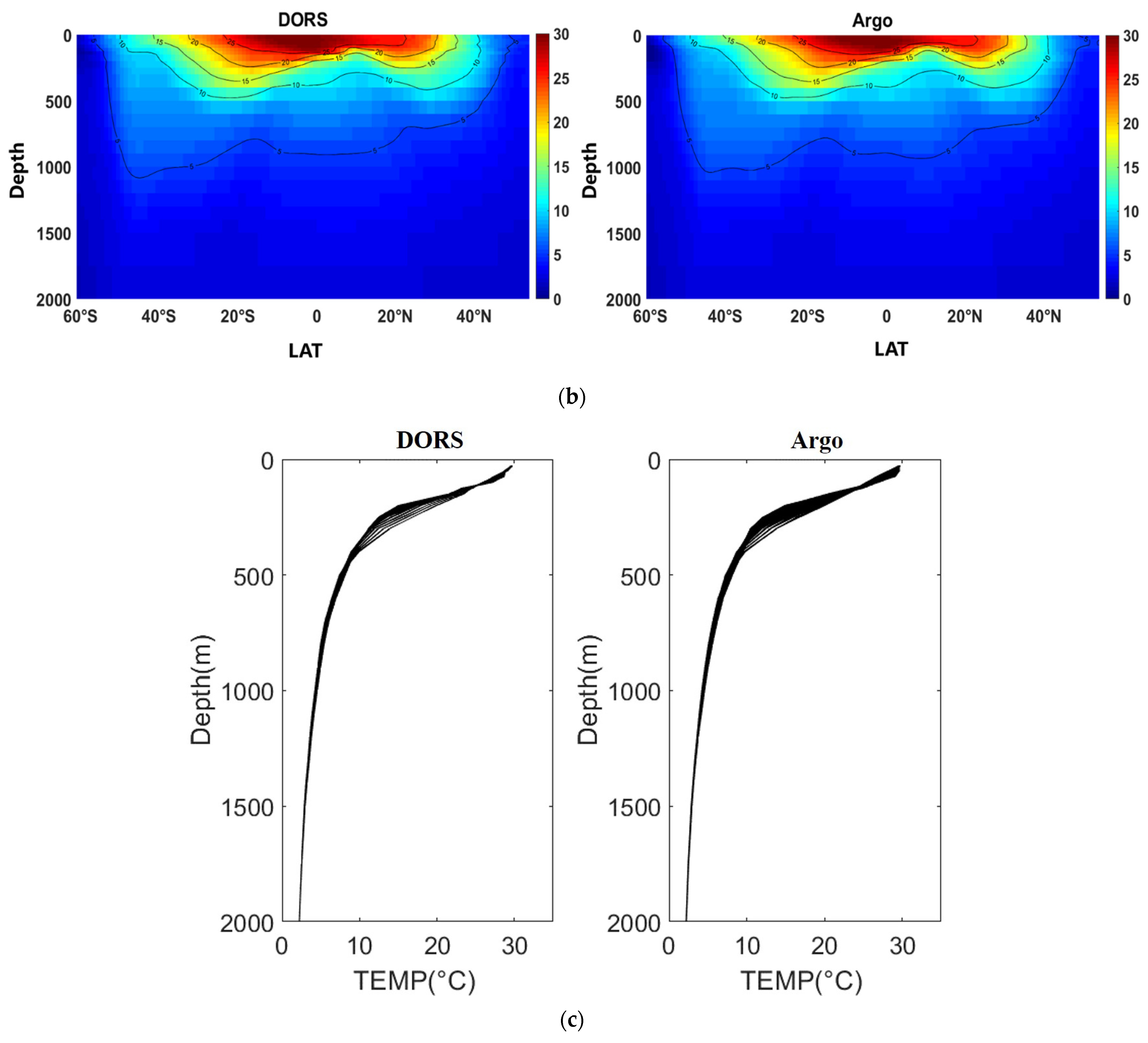
We compared and analyzed the temperature structure from the perspective of the 3D spatial form and distribution pattern to thoroughly verify the pros and cons of the DORS dataset. Figure 9a depicts the spatial distribution of SST in the global ocean in January 2016, from which meridian section A and rectangular section B are intercepted, and the length and width of the matrix are 10. Figure 9b depicts the meridional section of the DORS and Argo datasets at a longitude of 160°W. The result indicates that the vertical temperature structure presents a gradual decrease trend from the surface to the subsurface and deep ocean. The high temperature south of the Equator vertically extends deeper than north of the Equator, which may be related to season variability. The high-temperature zone is mainly concentrated between 30°S–30°N, and the temperature changes significantly in the range of 0–500 m. Temperature fluctuation below 500 m tends to be stable, with a small range of change. The DORS isotherms are relatively smooth, and the data transitions in different layers are also relatively smooth. The overall spatial shape and trend of the DORS dataset are similar to those of the Argo dataset, indicating that the ConvLSTM reconstruction accuracy will not be significantly reduced as the depth increases.
Figure 9c depicts the vertical distribution of all grid points for DORS ST and Argo ST in rectangular area B in January 2016. Statistical analysis shows that more than 98.48% of the profile points for reconstruction have error less than ±1 °C, and more than 88.87% of the profile points for reconstruction have error less than ±0.5 °C. The temperature of the subsurface layer drops gently, and the temperature of the subsurface layer drops from about 30 °C to about 27 °C in this range. In the thermocline layer, the ST drops abruptly, while in the deep layer the ST keeps stable. The results show that the temperature distribution patterns of DORS and Argo are similar in all layers for the upper 2000 m, indicating that DORS has a high reconstruction quality.

4.3. Subsurface Temperature Evolution and Global Ocean Warming

4.3.1. Spatiotemporal Patterns from EOF Analysis

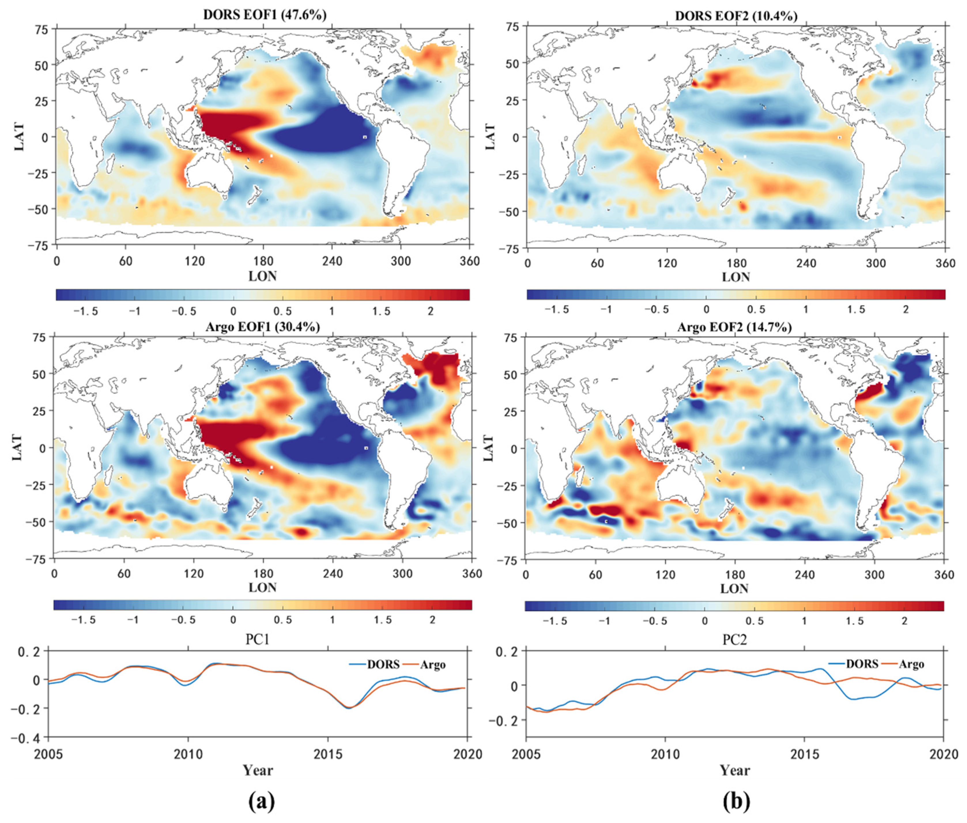
Empirical orthogonal function (EOF) analysis was performed on the DORS and Argo datasets to further demonstrate DORS’s ability to capture the spatiotemporal variability of ST. This study conducts an EOF analysis of the global temperature monthly product after removing linear trends and seasonal signals (using a 12-month moving average). Figure 10 depicts the comparative EOF analysis of the average temperature anomaly of 23 layers from 0 to 2000 m based on the DORS and Argo data. The spatial patterns of the DORS and Argo data are relatively consistent. The EOFs (spatial modes) and PCs (temporal coefficients) of the first two modes are shown in Figure 10, and the total variance contribution rates for the two modes are 58.0% (DORS) and 45.1% (Argo), respectively. In the first mode, the PCs of the two products match very well and differ only slightly (Figure 10a), and the EOFs are also very similar, particularly in the tropical Pacific. The majority of the differences only exist in the North Atlantic and the Southern Ocean, with Argo capturing more variation details in the latter. In the first mode, a strong ENSO-dominated dipole pattern in the tropical Pacific is presented, and there is also a dipole pattern around the tropical Indian Ocean (IO), indicating that DORS accurately captures the leading pattern of ocean temperature anomaly. There is a positive anomaly pattern and a negative anomaly pattern coexisting in the North Atlantic Ocean. The first PC shows strong interannual variability with a relatively stable trend for the time series temporal coefficient, which may be related to ENSO variability. The second mode demonstrates distinctive boundary currents and Antarctic Circumpolar Current (ACC) variations, and there are some pattern inconsistencies between DORS and Argo, with more prominent differences in the Atlantic Ocean and the Southern Ocean (SO), but the overall trends of temporal coefficients are similar with a slight increase trend (Figure 10b). In general, the ENSO variability and large-scale ocean circulations dominate the spatiotemporal pattern of the global subsurface temperature anomaly.

4.3.2. Subsurface Temperature Evolution Related to ENSO

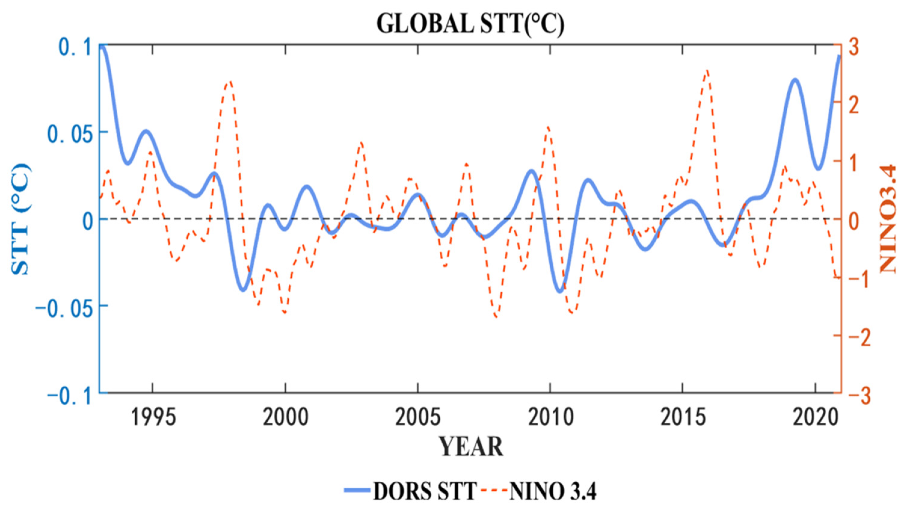
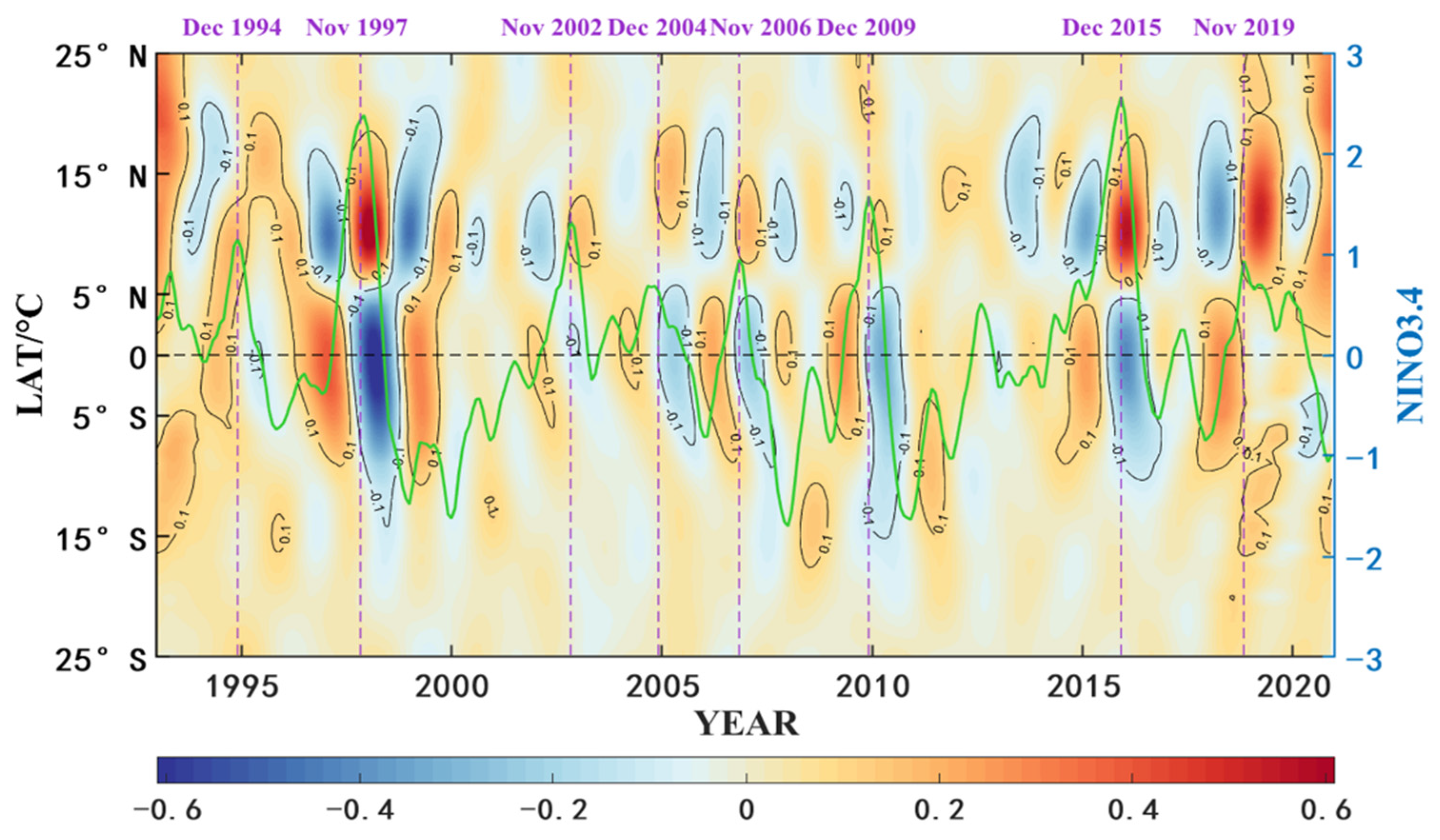
El Niño–Southern Oscillation (ENSO) is the dominant mode of air-sea interaction in the climate system. The spatial pattern of ocean temperature is greatly modulated by ENSO (Figure 10). To examine the subsurface temperature evolution related to ENSO, we calculated the subsurface temperature tendency (STT) using the central difference method based on the DORS dataset (using Lanczos filters and smoothing to reduce noise and the effects of decadal variability before calculation) [40]. The result indicated that global STT is negatively correlated with the NINO 3.4 index, that is, the ocean subsurface temperature shows a cooling trend during El Niño and a warming trend during La Niña. The relationship between STT and ENSO was well examined based on time series, and the global subsurface temperature showed a trend of cooling during the developmental stage of El Niño and reached a minimum value shortly after the peak of El Niño (Figure 11). This phenomenon can be easily observed in the years of several stronger El Niño events. In addition, it is found that the trend of ocean temperature change lags behind the development of ENSO events, such that observation of the development stages of ENSO events can make some simple projections of the trend of ocean temperature changes.
In addition, we also discuss the temperature changes in the tropics where ENSO events originate and analyze the spatial characteristics of temperature changes from the perspective of latitude. A Hovmöller diagram of the meridional-averaged STT in the upper 2000 m in the tropics from 1993 to 2020 shows the ENSO-related heat redistribution in and out of the equatorial zone (Figure 12). The southern and equatorial tropical oceans (15°S–5°N) tend to warm during La Niña and before El Niño (STT > 0) and cool during and after El Niño (STT < 0). There is an opposite temperature trend in the 5–25°N region, suggesting that heat losses from the southern tropics during El Niño are dumped to areas beyond the equator in the northern hemisphere. During the 1997–1998 and 2015–2016 super El Niño events, temperature trends in the tropics differed by more than 0.6 °C.

4.3.3. Subsurface Temperature Anomaly and Ocean Warming Trends

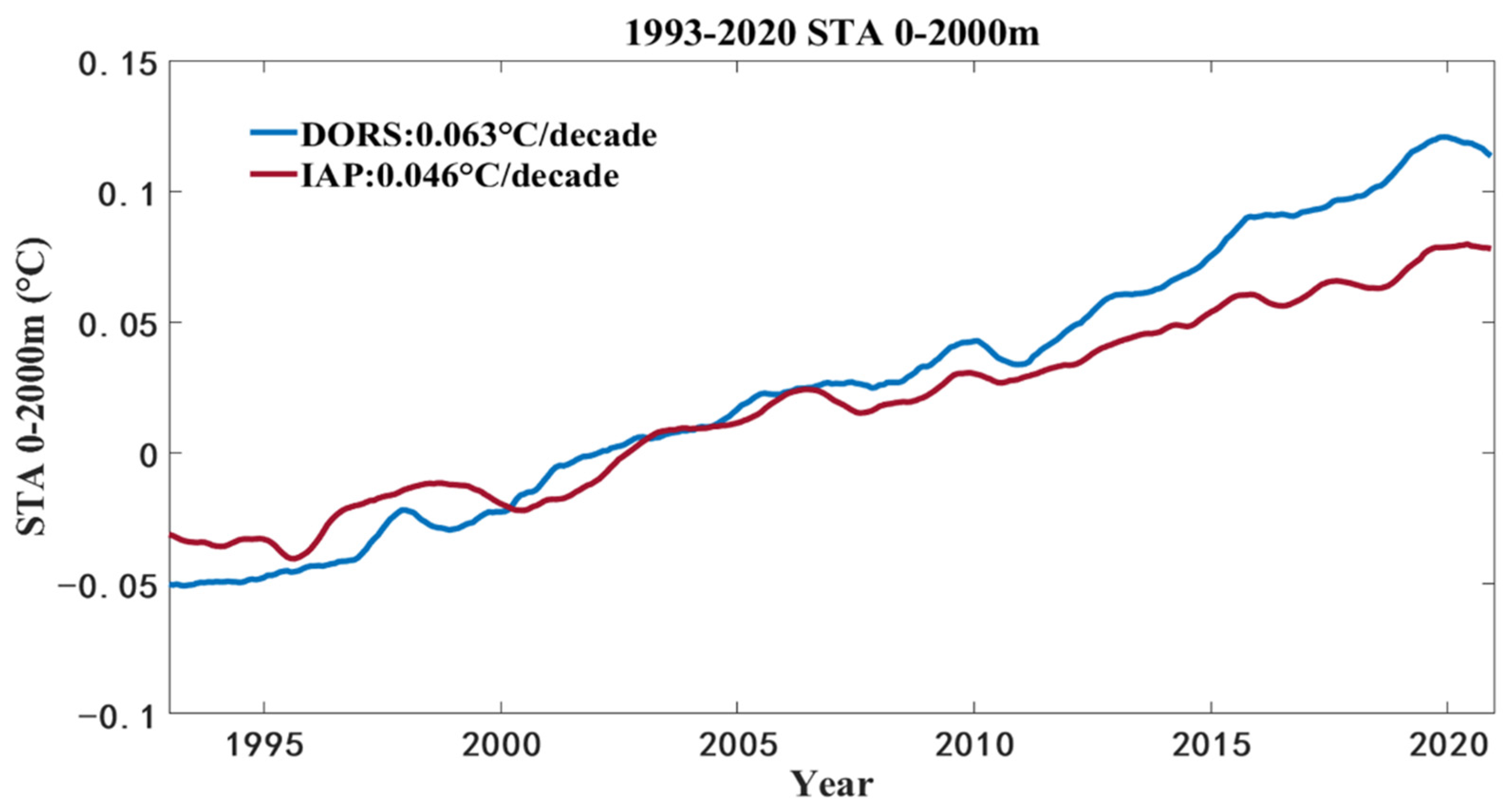
Based on the DORS dataset subtracts, the subsurface temperature anomaly (STA) and the spatiotemporal trends of ST in the global ocean and ocean basins are calculated (the time series is from 1993 to 2020, and the climatological baseline is from 1993 to 2012). Figure 13 shows the long-term STA evolution in the upper 2000 m of the global ocean based on DORS and IAP datasets. The linear trends for the global ocean ST at different layers and ocean basins from 1993 to 2020 are shown in Table 3. The ocean has warmed significantly since 1993, and the trends of STA for the upper 2000 m from 1993 to 2020 for the DORS and IAP datasets are 0.063 and 0.046 °C/decade, respectively (Figure 13). Although there are some differences in terms of trend, both trends are generally consistent and have the same order of magnitude. Some discrepancies in the trends are inevitable and acceptable because the existing gridded datasets based on optimal interpolation still have some uncertainties (interpolation error caused by the XBT systematic error and observation sparseness and unevenness), and the remote sensing projection and AI perspective for our DORS reconstruction are completely different from the existing gridded datasets.
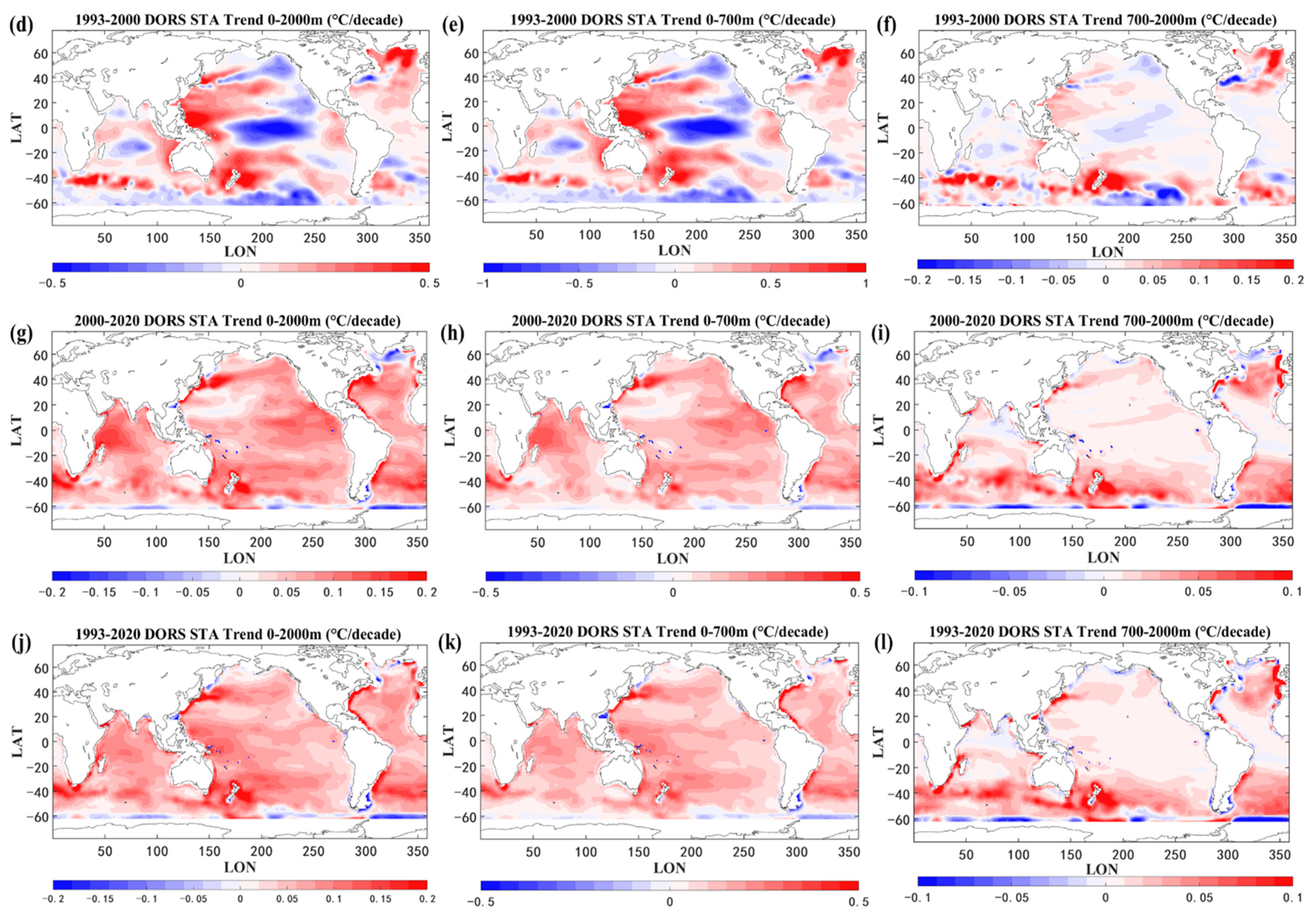
There was a slight warming in ocean temperature at the end of the 20th century, from 1993 to 2000. The global ocean temperature increased slowly before the 21st century (0.047 °C/decade), and the warming rate accelerated greatly after 2000 (0.064 °C/decade), especially in the deep ocean (0–700 m) with a direct transition from cooling to warming (0.127 °C/decade) (Figure 14d,g,i). The spatial distribution of the warming trend of the 0–700 m layer is close to that of the 0–2000 m layer, and the overall warming rate of the 0–700 m layer is higher than that of the 700–2000 m layer. The warming area of the global ocean temperature from 1993 to 2000 is predominantly focused on the equatorial western PO and part of the North Atlantic Ocean, as can be observed from the spatial distribution (Figure 14d). In the equatorial eastern Pacific Ocean and high-latitude waters of the SO, there is a relatively strong cooling phenomenon, and the ocean temperature change at the end of the 20th century was mainly affected by the 0–700 m layers (Figure 14d,e), while the 700–2000 m layers had little effect on the trend of ST (Figure 14f). After 2000, the global ocean showed a continuous warming trend, and the cooling trend was scattered in the high-latitude waters of the SO and the North Atlantic Ocean (Figure 14g,h,i). The global ocean boundary currents and the Antarctic Circumpolar Current show significant warming trends for the upper 2000 m (Figure 14j,h,l). Undoubtedly, the global ocean has been in a long-term warming trend since the start of the 21st century (Figure 14j), and the global ocean temperature is setting new records in recent years [7].
The temperature evolution trends at the ocean basin scale show significant spatial heterogeneity. The warming rates of the AO and the IO are similar at the 0–2000 m layers (Figure 14a), and the AO is in a state of rapid warming throughout the time series (0.074 °C/decade). The warming rate of the SO slowed down from 2005 to 2010; meanwhile, other ocean basins were on an accelerating warming trend. At the 0–700 m layer (Figure 14b), the overall warming rate of the AO was fast, and the rate of PO was higher than that of the IO. The warming rate of each ocean basin increased after 2000. In 2015, the IO showed a brief warming slowdown trend and then recovered quickly, possibly due to the influence of El Niño events. The PO was warming slowly (0.013 °C/decade) from 700 to 2000 m, which is lower than in the AO (0.022 °C/decade), the IO (0.025 °C/decade), and the SO (0.014 °C/decade). After 2005, the IO warming was considerably accelerated, while that in the SO fluctuated greatly. The warming rate of the SO was not fast, was relatively stable, and was in a state of warming most of the time, and the warming rate of deep ocean water greatly accelerated from 2010 to 2015 (Figure 14c).
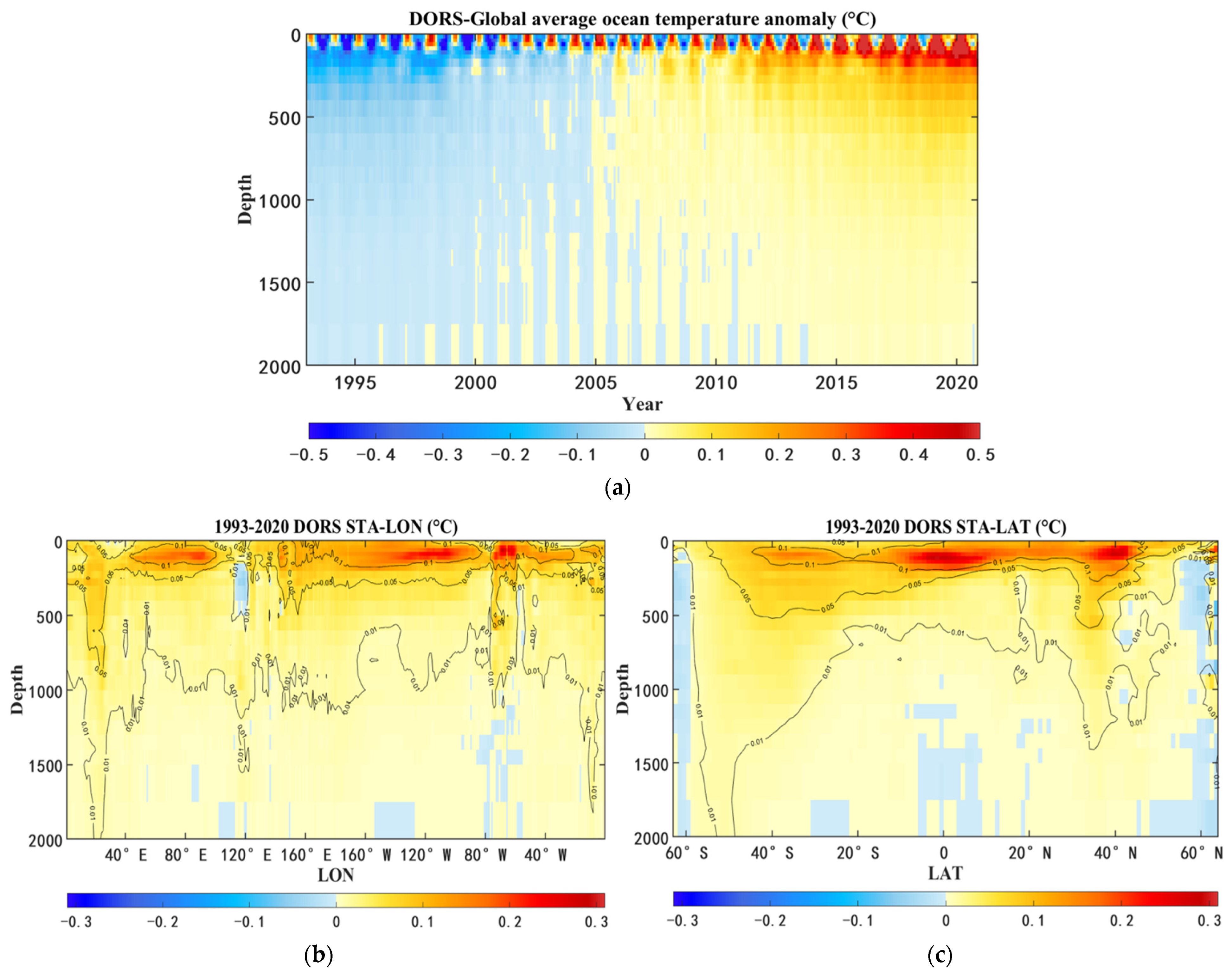
The vertical long-term evolution of global ocean temperature was examined to investigate the tendency of the global ocean temperature anomaly from a vertical perspective. The global ocean surface showed an alternation of cooling and warming from 1993 to 2020, primarily due to the ENSO event as illustrated in Figure 15a, and the surface warming became more and more significant with time. Ocean warming gradually progressed from the ocean surface to the deep layer after 2005. The warming trend of the deep ocean was not significant before 2005, but after 2005, excepting the surface, a warming trend in the 100–2000 m layer was observed. The results showed that the interior of the ocean is in a state of continuous warming, and global ocean warming gradually extends to the deep ocean.
We divide the global profile into the meridional and zonal directions (Figure 15b,c) to investigate the variation trend of ocean temperature in the meridional and latitudinal directions, with a profile depth of 0–2000 m. Using the zonal average of the global ocean to obtain a meridional profile, it can be found that the DORS dataset can well demonstrate the trend of global ocean warming from the surface to the deep ocean. Above 1000 m, the seawater at almost all longitudes in the world is in a warming trend, and below 1000 m, there are also warming signals near the IO and the AO, which is consistent with previous studies (Figure 15b). Similarly, to obtain a zonal profile, the global ocean is averaged in the meridional direction, and the variation trend of ocean temperature in the zonal profile is analyzed (Figure 15c). From the profile distribution displayed by DORS STA, it is not difficult to see that the deep warming in the Southern Hemisphere is more pronounced in high latitudes than in low latitudes, especially in the SO, and there is a slight cooling trend of ST in the high latitudes of the Northern Hemisphere.

5. Conclusions

In this study, we established a time series reconstruction model of global ocean ST and produced a new global ocean ST product (DORS) based on the ConvLSTM algorithm. The network model makes up for the insufficiency of LSTM in processing spatiotemporal data, and can effectively learn the spatiotemporal variation characteristics of marine data. Moreover, we also adopted an advanced ensemble learning LighGBM for model comparison; the results demonstrated that the ConvLSTM model outperformed the LighGBM model for the data reconstruction. This study quantitatively evaluates the reconstruction accuracy of the DORS dataset from multiple perspectives. Based on the DORS dataset, we effectively track the global ocean warming in the upper 2000 m for about three decades from 1993 to 2020 and carry out spatiotemporal analysis of global ocean temperature to examine and understand the spatial patterns, evolution trends, and vertical characteristics of global ST changes.
The results suggest that: (1) the reconstructed DORS dataset based on the ConvLSTM model has a high correlation with well-used international ocean datasets. The R2 with Argo, IAP, EN4, Ishii, and ARMOR3D is 0.99/0.98/0.98/0.99/0.98, and the RMSE is 0.34 °C/0.46 °C/0.53 °C/0.44 °C/0.57 °C. The average R2 and NRMSE validated by the EN4-Profile dataset over time series are 0.94/0.05 °C, suggesting that our DORS dataset is reliable with high accuracy. In terms of 3D spatial morphology and distribution pattern, the DORS temperature structure matches well with the Argo data. It proves that the ConvLSTM network can, indeed, successfully capture and learn the spatiotemporal features of ocean observation data. (2) The ST spatiotemporal modes from the EOF analysis indicate that DORS correctly captures the leading mode of ocean temperature. The STT is negatively correlated with the NINO 3.4 index, and there is significant heat transfer in the tropics. The spatial pattern of global STT is greatly influenced by the ENSO variability. (3) There are significant differences in ocean temperature evolution trends between the end of the 20th century and the first two decades of the 21st century. Compared to the warming rate before 2000 (0.047 °C/decade), the warming rate after 2000 was greatly increased (0.064 °C/decade). There are also some differences for the warming trends in different ocean basins and depth layers, and the warming signal in the subsurface and deeper ocean (300–2000 m) has become more significant, which suggests that the subsurface and deeper ocean plays a more and more important role in heat uptake and storage. There is a distinctive and continuous warming process within the ocean, and the warming signal prominently extends from the upper layer to the subsurface and deeper layer during recent global warming.
Overall, from a remote sensing perspective, the DORS product can well fill the gap in the pre-Argo era and provide new and robust data support for ocean interior process and climate change studies. The time series reconstruction of the global ocean ST structure above 2000 m is currently limited to 1° × 1° due to the limitation of the Argo data resolution. However, with the development of artificial intelligence technology and the gradual enrichment of observation methods in the ocean, it will be possible to reconstruct the 3D temperature structure of higher resolution, deeper layers, and longer time series. The establishment of the DORS product is not only a supplement to the ocean datasets. Based on the DORS product, we further examine and understand the spatial patterns, evolution trends, and vertical characteristics of global ST changes. In the future, the DORS product will continue to be supported for global ocean temperature anomaly and ocean heat content change analysis, and other marine climate change and variability studies, and provide valuable and promising data support for ocean dynamic process, global warming, and Sustainable Development Goals (SDGs).

Author Contributions

Conceptualization, H.S.; methodology, J.J.; validation, J.J. and A.W.; formal analysis, H.S. and J.J.; investigation, H.S. and A.W.; data curation, J.J.; writing—original draft preparation, H.S. and J.J.; writing—review and editing, H.S. and W.Z.; visualization, J.J. and A.W.; supervision, H.S., W.Z. and X.-H.Y.; funding acquisition, H.S. and X.-H.Y. All authors have read and agreed to the published version of the manuscript.

Funding

This research was funded by the National Natural Science Foundation of China (41971384), the Natural Science Foundation for Distinguished Young Scholars of Fujian Province of China (2021J06014), the National Key R&D Program of China (2019YFA0606702), and the National Natural Science Foundation of China (91858202).

Institutional Review Board Statement

Not applicable.

Informed Consent Statement

Not applicable.

Data Availability Statement

The data presented in this study are available on request from the corresponding author.

Acknowledgments

The authors would like to thank three anonymous reviewers for their helpful comments, which significantly improved the quality of our paper. The DORS dataset has been shared to the research community at Science Data Bank (ScienceDB) and can be freely accessed (http://www.doi.org/10.57760/sciencedb.01918, accessed on 1 April 2022).

Conflicts of Interest

The authors declare no conflict of interest.

References

  1. Von Schuckmann, K.; Cheng, L.; Palmer, M.D.; Hansen, J.; Tassone, C.; Aich, V.; Adusumilli, S.; Beltrami, H.; Boyer, T.; Cuesta-Valero, F.J. Heat stored in the Earth system: Where does the energy go? Earth Syst. Sci. Data 2020, 12, 2013–2041. [Google Scholar] [CrossRef]
  2. Wouters, B.; van de Wal, R. Global sea-level budget 1993--present. Earth Syst. Sci. Data 2018, 10, 1551–1590. [Google Scholar]
  3. Meyssignac, B.; Boyer, T.; Zhao, Z.; Hakuba, M.Z.; Landerer, F.W.; Stammer, D.; Köhl, A.; Kato, S.; L Ecuyer, T.; Ablain, M. Measuring global ocean heat content to estimate the Earth energy imbalance. Front. Mar. Sci. 2019, 6, 432. [Google Scholar] [CrossRef] [Green Version]
  4. Von Schuckmann, K.; Palmer, M.D.; Trenberth, K.E.; Cazenave, A.; Chambers, D.; Champollion, N.; Hansen, J.; Josey, S.A.; Loeb, N.; Mathieu, P. An imperative to monitor Earth’s energy imbalance. Nat. Clim. Chang. 2016, 6, 138–144. [Google Scholar] [CrossRef] [Green Version]
  5. Yan, X.H.; Boyer, T.; Trenberth, K.; Karl, T.R.; Xie, S.P.; Nieves, V.; Tung, K.K.; Roemmich, D. The global warming hiatus: Slowdown or redistribution? Earth’s Future 2016, 4, 472–482. [Google Scholar] [CrossRef]
  6. Cheng, L.; Trenberth, K.E.; Fasullo, J.; Boyer, T.; Abraham, J.; Zhu, J. Improved estimates of ocean heat content from 1960 to 2015. Sci. Adv. 2017, 3, e1601545. [Google Scholar] [CrossRef] [Green Version]
  7. Cheng, L.; Abraham, J.; Zhu, J.; Trenberth, K.E.; Fasullo, J.; Boyer, T.; Locarnini, R.; Zhang, B.; Yu, F.; Wan, L.; et al. Record-Setting Ocean Warmth Continued in 2019. Adv. Atmos. Sci. 2020, 37, 137–142. [Google Scholar] [CrossRef] [Green Version]
  8. Cheng, L.; Zhu, J. Uncertainties of the ocean heat content estimation induced by insufficient vertical resolution of historical ocean subsurface observations. J. Atmos. Ocean. Technol. 2014, 31, 1383–1396. [Google Scholar] [CrossRef]
  9. Wang, G.; Cheng, L.; Abraham, J.; Li, C. Consensuses and discrepancies of basin-scale ocean heat content changes in different ocean analyses. Clim. Dynam. 2018, 50, 2471–2487. [Google Scholar]
  10. Dickey, T.D. Emerging ocean observations for interdisciplinary data assimilation systems. J. Mar. Syst. 2003, 40, 5–48. [Google Scholar] [CrossRef]
  11. Talley, L.D.; Pickard, G.L.; Emery, W.J.; Swift, J.H. Dynamical processes for descriptive ocean circulation. Descr. Phys. Oceanogr. 2011, 6, 187–259. [Google Scholar]
  12. Klein, S.A.; Soden, B.J.; Lau, N. Remote sea surface temperature variations during ENSO: Evidence for a tropical atmospheric bridge. J. Clim. 1999, 12, 917–932. [Google Scholar] [CrossRef] [Green Version]
  13. Martin, S. An Introduction to Ocean Remote Sensing; Cambridge University Press: New York, NY, USA, 2014. [Google Scholar]
  14. Ali, M.M.; Swain, D.; Weller, R.A. Estimation of ocean subsurface thermal structure from surface parameters: A neural network approach. Geophys. Res. Lett. 2004, 31, L20308. [Google Scholar] [CrossRef] [Green Version]
  15. Klemas, V.; Yan, X. Subsurface and deeper ocean remote sensing from satellites: An overview and new results. Prog. Oceanogr. 2014, 122, 1–9. [Google Scholar] [CrossRef]
  16. Wang, J.; Flierl, G.R.; LaCasce, J.H.; McClean, J.L.; Mahadevan, A. Reconstructing the ocean′s interior from surface data. J. Phys. Oceanogr. 2013, 43, 1611–1626. [Google Scholar] [CrossRef]
  17. Su, H.; Wu, X.; Yan, X.; Kidwell, A. Estimation of subsurface temperature anomaly in the Indian Ocean during recent global surface warming hiatus from satellite measurements: A support vector machine approach. Remote Sens. Environ. 2015, 160, 63–71. [Google Scholar] [CrossRef]
  18. Cheng, L.; Zhu, J. Benefits of CMIP5 multimodel ensemble in reconstructing historical ocean subsurface temperature variations. J. Clim. 2016, 29, 5393–5416. [Google Scholar] [CrossRef]
  19. Guinehut, S.; Dhomps, A.; Larnicol, G.; Le Traon, P. High resolution 3-D temperature and salinity fields derived from in situ and satellite observations. Ocean. Sci. 2012, 8, 845–857. [Google Scholar] [CrossRef] [Green Version]
  20. Su, H.; Huang, L.; Li, W.; Yang, X.; Yan, X.H. Retrieving ocean subsurface temperature using a satellite-based geographically weighted regression model. J. Geophys. Res. Ocean. 2018, 123, 5180–5193. [Google Scholar] [CrossRef]
  21. Yu, F.; Wang, Z.; Liu, S.; Chen, G. Inversion of the three-dimensional temperature structure of mesoscale eddies in the Northwest Pacific based on deep learning. Acta Oceanol. Sin. 2021, 40, 176–186. [Google Scholar] [CrossRef]
  22. Akbari, E.; Alavipanah, S.K.; Jeihouni, M.; Hajeb, M.; Haase, D.; Alavipanah, S. A review of ocean/sea subsurface water temperature studies from remote sensing and non-remote sensing methods. Water 2017, 9, 936. [Google Scholar] [CrossRef] [Green Version]
  23. Su, H.; Li, W.; Yan, X.H. Retrieving temperature anomaly in the global subsurface and deeper ocean from satellite observations. J. Geophys. Res. Ocean. 2018, 123, 399–410. [Google Scholar] [CrossRef]
  24. Su, H.; Yang, X.; Lu, W.; Yan, X. Estimating subsurface thermohaline structure of the global ocean using surface remote sensing observations. Remote Sens. 2019, 11, 1598. [Google Scholar] [CrossRef] [Green Version]
  25. Wang, H.; Song, T.; Zhu, S.; Yang, S.; Feng, L. Subsurface temperature estimation from sea surface data using neural network models in the western pacific ocean. Mathematics 2021, 9, 852. [Google Scholar] [CrossRef]
  26. Bolton, T.; Zanna, L. Applications of deep learning to ocean data inference and subgrid parameterization. J. Adv. Model. Earth Syst. 2019, 11, 376–399. [Google Scholar]
  27. Ham, Y.; Kim, J.; Luo, J. Deep learning for multi-year ENSO forecasts. Nature 2019, 573, 568–572. [Google Scholar] [CrossRef]
  28. Meng, L.; Yan, C.; Zhuang, W.; Zhang, W.; Geng, X.; Yan, X. Reconstructing High-Resolution Ocean Subsurface and Interior Temperature and Salinity Anomalies From Satellite Observations. IEEE Trans. Geosci. Remote Sens. 2021, 99, 1–14. [Google Scholar] [CrossRef]
  29. Zuo, X.; Zhou, X.; Guo, D.; Li, S.; Liu, S.; Xu, C. Ocean Temperature Prediction Based on Stereo Spatial and Temporal 4-D Convolution Model. IEEE Geosci. Remote Sens. Lett. 2021, 19, 1–5. [Google Scholar] [CrossRef]
  30. Su, H.; Zhang, T.; Lin, M.; Lu, W.; Yan, X. Predicting subsurface thermohaline structure from remote sensing data based on long short-term memory neural networks. Remote Sens. Environ. 2021, 260, 112465. [Google Scholar]
  31. Jiang, F.; Ma, J.; Wang, B.; Shen, F.; Yuan, L. Ocean Observation Data Prediction for Argo Data Quality Control Using Deep Bidirectional LSTM Network. Secur. Commun. Netw. 2021, 2021, 5665386. [Google Scholar] [CrossRef]
  32. Liu, J.; Zhang, T.; Han, G.; Gou, Y. TD-LSTM: Temporal dependence-based LSTM networks for marine temperature prediction. Sensors 2018, 18, 3797. [Google Scholar] [CrossRef] [PubMed] [Green Version]
  33. Contractor, S.; Roughan, M. Efficacy of feedforward and lstm neural networks at predicting and gap filling coastal ocean timeseries: Oxygen, nutrients, and temperature. Front. Mar. Sci. 2021, 8. [Google Scholar] [CrossRef]
  34. Su, H.; Qin, T.; Wang, A.; Lu, W. Reconstructing ocean heat content for revisiting global ocean warming from remote sensing perspectives. Remote Sens. 2021, 13, 3799. [Google Scholar] [CrossRef]
  35. Shi, X.; Chen, Z.; Wang, H.; Yeung, D.; Wong, W.; Woo, W. Convolutional LSTM network: A machine learning approach for precipitation nowcasting. Adv. Neural Inf. Processing Syst. 2015, 28, 802–810. [Google Scholar]
  36. Good, S.A.; Martin, M.J.; Rayner, N.A. EN4: Quality controlled ocean temperature and salinity profiles and monthly objective analyses with uncertainty estimates. J. Geophys. Res. Ocean. 2013, 118, 6704–6716. [Google Scholar] [CrossRef]
  37. Ishii, M.; Fukuda, Y.; Hirahara, S.; Yasui, S.; Suzuki, T.; Sato, K. Accuracy of global upper ocean heat content estimation expected from present observational data sets. SOLA 2017, 13, 163–167. [Google Scholar] [CrossRef] [Green Version]
  38. Ke, G.; Meng, Q.; Finley, T.; Wang, T.; Chen, W.; Ma, W.; Ye, Q.; Liu, T. Lightgbm: A highly efficient gradient boosting decision tree. Adv. Neural Inf. Processing Syst. 2017, 30, 3149–3157. [Google Scholar]
  39. Zhang, T.Y.; Su, H.; Yang, X.; Yan, X.-H. Remote sensing prediction of global subsurface thermohaline and the impact of longitude and latitude based on LightGBM. J. Remote Sens. 2020, 24, 1255–1269. [Google Scholar]
  40. Cheng, L.; Trenberth, K.E.; Fasullo, J.T.; Mayer, M.; Balmaseda, M.; Zhu, J. Evolution of ocean heat content related to ENSO. J. Clim. 2019, 32, 3529–3556. [Google Scholar] [CrossRef]
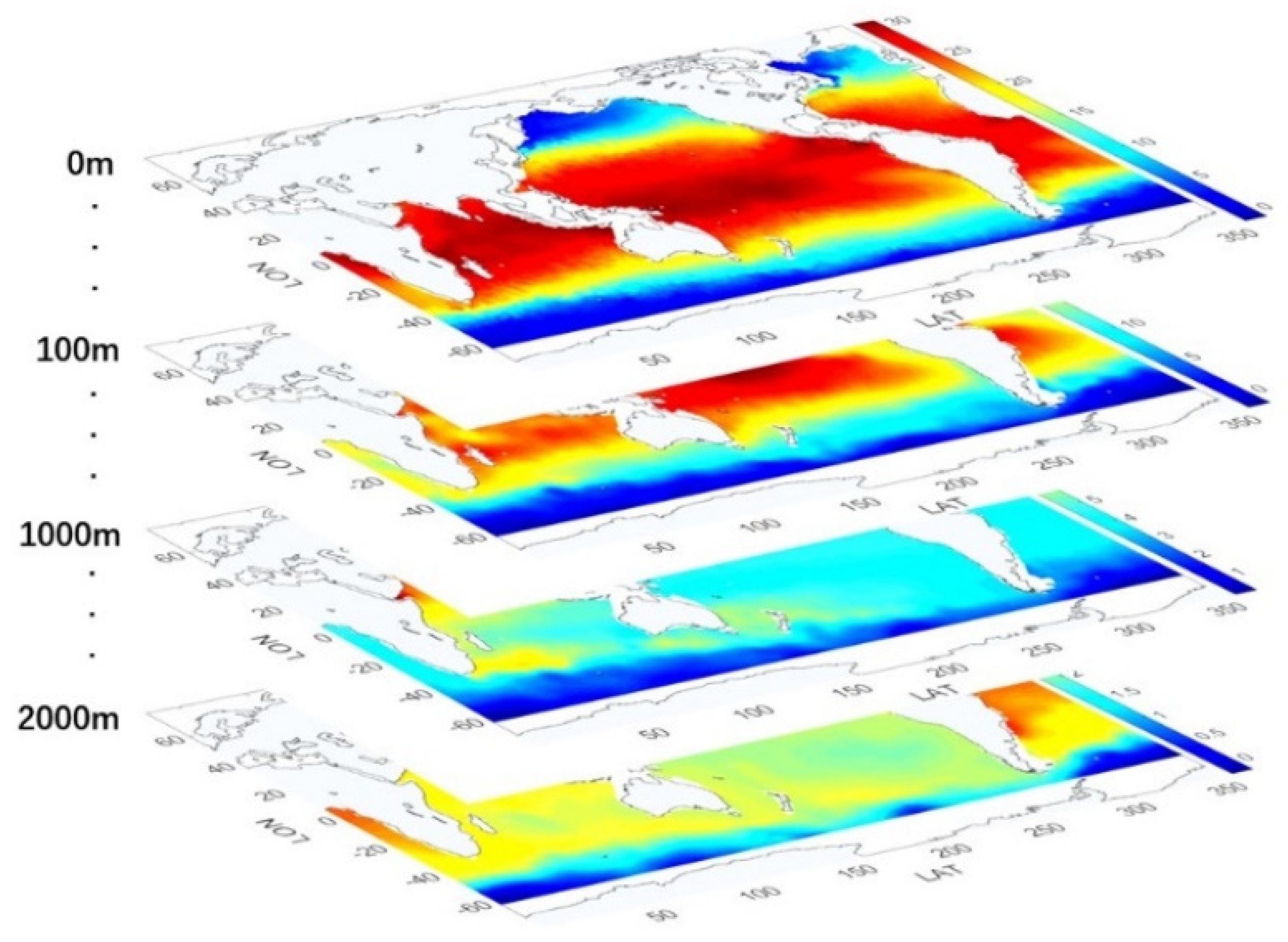
Figure 1. Technical flowchart for satellite-based time series reconstruction of global subsurface temperature based on the ConvLSTM model.
Remotesensing 14 03198 g001
Figure 2. Technical flowchart for satellite-based time series reconstruction of global subsurface temperature based on the ConvLSTM model.
Remotesensing 14 03198 g002
Figure 3. The R2 and NRMSE for ConvLSTM and LightGBM validated by EN4-Profile dataset at different depth levels.
Remotesensing 14 03198 g003
Figure 4. (a) Time series mean R2 and RMSE at different depths for DORS relative to the Argo, IAP, EN4, Ishii, and ARMOR3D datasets. (b) Depth-averaged R2 of DORS relative to the Argo (from 2005 to 2019), IAP, EN4, Ishii, and ARMOR3D datasets over long time series. (c) The R2 and NRMSE at different depths in the upper 2000 m validated by the EN4-Profile dataset from 1993 to 2020. The lines in the figure were smoothed by running a mean filter for 6 months.
Remotesensing 14 03198 g004aRemotesensing 14 03198 g004b
Figure 5. The spatial distributions of DORS, LightGBM, and Argo at 100 m for January 2016, and intensity scatter plots: (a) is the LightGBM ST, (b) is the DORS ST, (c) is the intensity scatter plots between the LightGBM ST and the EN4-Profile ST, (d) is the Argo ST, and (e) is the intensity scatter plots between the DORS ST and the EN4-Profile ST.
Remotesensing 14 03198 g005
Figure 6. The spatial distribution of DORS, LightGBM, and Argo at 500 m for January 2016, and intensity scatter plots: (a) is the LightGBM ST, (b) is the DORS ST, (c) is the intensity scatter plots between the LightGBM ST and the EN4-Profile ST, (d) is the Argo ST, and (e) is the intensity scatter plots between the DORS ST and the EN4-Profile ST.
Remotesensing 14 03198 g006
Figure 7. The spatial distribution of DORS, LightGBM, and Argo at 1000 m for January 2016, and intensity scatter plots: (a) is the LightGBM ST, (b) is the DORS ST, (c) is the intensity scatter plots between the LightGBM ST and the EN4-Profile ST, (d) is the Argo ST, and (e) is the intensity scatter plots between the DORS ST and the EN4-Profile ST.
Remotesensing 14 03198 g007
Figure 8. The spatial distribution of DORS, LightGBM, and Argo at 2000 m for January 2016, and intensity scatter plots: (a) is the LightGBM ST, (b) is the DORS ST, (c) is the intensity scatter plots between the LightGBM ST and the EN4-Profile ST, (d) is the Argo ST, and (e) is the intensity scatter plots between the DORS ST and the EN4-Profile ST.
Remotesensing 14 03198 g008
Figure 9. (a) Spatial distribution of sea surface temperature (SST) in the global ocean in January 2016. A meridional profile A (longitude of 160°W) and a rectangular profile B were intercepted in the figure to analyze the vertical variation of ST. (b) The meridional vertical distribution of Argo ST and DORS ST in January 2016 where the longitude is 160°W. (c) Vertical profile of all grid points in rectangular area B for DORS ST and Argo ST in January 2016.
Remotesensing 14 03198 g009aRemotesensing 14 03198 g009b
Figure 10. Comparative EOF analysis of the average temperature anomaly in the upper 2000 m from 2005 to 2019 based on DORS and Argo data (baseline: 2005–2015). (a) The first spatial mode and respective temporal coefficient (PC1 for DORS and Argo); (b) the second spatial mode and respective temporal coefficient (PC2 for DORS and Argo). The lines in the figure were smoothed by running a mean filter for 12 months.
Remotesensing 14 03198 g010
Figure 11. Time series evolutions of DORS STT and the NINO 3.4 index from 1993–2020.
Remotesensing 14 03198 g011
Figure 12. A Hovmöller diagram of the STT obtained by meridional averaging over the 25°S–25°N tropics based on the DORS dataset, along with the evolution of the NINO 3.4 index (green) (peaks of El Niño events since 1993 are marked with vertical dashed lines). The lines in the figure were smoothed by running a mean filter for 12 months.
Remotesensing 14 03198 g012
Figure 13. Monthly STA time series in the upper 2000 m of the global ocean from the DORS and IAP datasets from 1993 to 2020. The baseline is from 1993 to 2012. Unit: °C. The lines in the figure were smoothed by running a mean filter for 12 months.
Remotesensing 14 03198 g013
Figure 14. (ac) Long-term time series trends of the global ocean and ocean-basin-scale subsurface temperature anomaly ((a) 0–2000 m, (b) 0–700 m, (c) 700–2000 m). (di) Spatial distribution patterns of global ocean temperature variation trends at different layers in the late 20th century and since the 21st century. (jl) Spatial distribution patterns of global ocean temperature variation trends at different layers from 1993 to 2020. The lines in the figure were smoothed by running a mean filter for 12 months.
Remotesensing 14 03198 g014aRemotesensing 14 03198 g014b
Figure 15. (a) Long-term change in the global ocean temperature vertical profile. (b) Long-term meridional profile change in global ocean temperature. (c) Long-term zonal profile change in global ocean temperature.
Remotesensing 14 03198 g015
Table 1. Data used in this study.
DataSourcesTimeSpatial Resolution
SSHhttp://www.aviso.altimetry.fr (accessed on 1 April 2021)1993–0.25° × 0.25°
SSThttps://www.ncei.noaa.gov/products/optimum-interpolation-sst (accessed on 1 April 2021)1981–0.25° × 0.25°
SSWhttps://rda.ucar.edu/datasets/ds745.1/ (accessed on 1 April 2021)1987–0.25° × 0.25°
Argohttp://apdrc.soest.hawaii.edu/projects/Argo/ (accessed on 1 April 2021)2005–1° × 1°
IAPhttp://159.226.119.60/cheng/ (accessed on 1 June 2021)1940–1° × 1°
EN4https://www.metoffice.gov.uk/hadobs/en4/ (accessed on 1 June 2021)1900–1° × 1°
EN4-Profilehttps://www.metoffice.gov.uk/hadobs/en4/ (accessed on accessed on 1 April 2022)1900–
Ishiihttps://climate.mri-jma.go.jp/pub/ocean/ts/v7.3.1 (accessed on 1 July 2021)1955–1° × 1°
ARMOR3Dhttps://resources.marine.copernicus.eu/product-detail/ (accessed on 15 July 2021)1993–0.25° × 0.25°
Table 2. ConvLSTM network parameters.
Network ParametersOptimal Parameters
Loss functionMean-squared-error
OptimizerRMSprop
ActivationELU
Learning rate0.001
Training samples413,881
Epoch4000
Table 3. Warming rates of the global ocean ST at different layers and ocean basins from 1993–2020 in ×°C/decade.
DepthsGlobalGlobal
(1993 to 1999)
Global
(2000 to 2020)
AOPOIOSO
0–700 m0.1230.0890.1270.1440.1380.1370.036
700–2000 m0.0170.0160.0170.0220.0130.0250.014
0–2000 m0.0630.0470.0640.0740.0680.0730.024
Publisher’s Note: MDPI stays neutral with regard to jurisdictional claims in published maps and institutional affiliations.