Article

Quality Control for the BPG Lossy Compression of Three-Channel Remote Sensing Images

1
Key Laboratory of Opto-Electronic Information Science and Technology of Jiangxi Province, Nanchang Hangkong University, Nanchang 330063, China
2
Department of Information and Communication Technologies, National Aerospace University, 61070 Kharkiv, Ukraine
3
Department of Signal Processing and Multimedia Engineering, West Pomeranian University of Technology, 70-313 Szczecin, Poland
*
Author to whom correspondence should be addressed.
Remote Sens. 2022, 14(8), 1824; https://doi.org/10.3390/rs14081824
Submission received: 24 February 2022 / Revised: 6 April 2022 / Accepted: 8 April 2022 / Published: 10 April 2022

Abstract

:
This paper deals with providing the desired quality in the Better Portable Graphics (BPG)-based lossy compression of color and three-channel remote sensing (RS) images. Quality is described by the Mean Deviation Similarity Index (MDSI), which is proven to be one of the best metrics for characterizing compressed image quality due to its high conventional and rank-order correlation with the Mean Opinion Score (MOS) values. The MDSI properties are studied and three main areas of interest are determined. It is shown that quite different quality and compression ratios (CR) can be observed for the same values of the quality parameter Q that controls compression, depending on the compressed image complexity. To provide the desired quality, a modified two-step procedure is proposed and tested. It has a preliminary stage carried out offline (in advance). At this stage, an average rate-distortion curve (MDSI on Q) is obtained and it is available until the moment when a given image has to be compressed. Then, in the first step, an image is compressed using the starting Q determined from the average rate-distortion curve for the desired MDSI. After this, the image is decompressed and the produced MDSI is calculated. In the second step, if necessary, the parameter Q is corrected using the average rate-distortion curve, and the image is compressed with the corrected Q. Such a procedure allows a decrease in the MDSI variance by around one order after two steps compared to variance after the first step. This is important for the MDSI of approximately 0.2–0.25 corresponding to the distortion invisibility threshold. The BPG performance comparison to some other coders is performed and examples of its application to real-life RS images are presented.

Graphical Abstract

1. Introduction

A general tendency in modern remote sensing (RS) imaging is to acquire data with higher resolution, for larger territories and more frequently [1]. This leads to collecting data having a very large size and running into typical problems of big data, i.e., difficulties with image processing, transferring, storage, and dissemination [2]. These difficulties with the RS data can be partially solved by their compression [3]. As is widely known, there are lossless and lossy image compression techniques that may be applied for general-purpose images [4]. The former group of methods allows original (undistorted) data to be obtained after decompression. However, in this case, the compression ratio (CR) is relatively small (limited by image entropy) and may reach values of around 5:1 only for hyper-spectral images with very high inter-band correlation [5]. Nevertheless, a larger CR is often needed in practical applications, particularly for RS images; hence, the only possibility is the use of lossy compression with inevitable distortions [6].
An interesting analysis of the influence of the lossy compression on the quality of aerial images using a weighted combination of qualitative parameters is presented in the paper [7], where the multi-criteria decision-making framework has been proposed for quality evaluation. Although there are many different requirements for lossy compression, their priority and type (obligatory or desired) usually depend on the application [8], e.g., there may be an initial condition to provide the minimum required CR. This may happen if a channel bandwidth and/or time of data transferring are limited. In such a situation, a coder should provide a simple way to define the desired CR (similarly to JPEG2000-like methods) and diminish introduced distortions to prevent their negative influence on further image processing, as well as the results of image analysis or classification studied in the paper [9] and object recognition effectiveness depending on the RS image quality [10]. For multi-channel data (e.g., color, multi-spectral, hyper-spectral), the compression performance may be improved by a preliminary decorrelation and the use of three-dimensional (3D) approaches for compression [11,12,13]. Another recent direction of research is the application of deep neural networks for the optimization of observer-dependent image compression towards a trade-off between the human visual system and classification accuracy [14]. However, in some applications, there may be another priority related to the introduced distortions (characterized by a specified measure or metric) below a given level, keeping the highest possible CR. Some of the issues may be related to the fast and efficient control (providing) of distortions’ level [15], and the choice of an adequate metric to characterize distortions, considering a task to be further solved using compressed data [16]. Some additional requirements may concern a certain format (according to some standards), compression speed, or, e.g., limited power consumption [17].
To satisfy the above requirements concerning the metrics, some pre-requisites have appeared recently, and considerable attention has been paid to metrics able to characterize the quality of RS data [16,18,19], including the artificial visible-like images based on SAR data generated with the use of deep CNNs [20]. In particular, special attention has been paid to the so-called visually lossless compression for RS image browsing and other applications [12,13,21,22,23]. This is important since compressed RS images are often subject to visual inspection. Meanwhile, JPEG2000 is not the best compression technique, similarly to the well-known full-reference image quality metric SSIM used in [12,13], which is clearly not the best among existing visual quality metrics. Perceptual quality has also received attention in the papers [24,25]. The necessity to provide a desired compression ratio and quality quickly enough is important in practical applications where processing time and resources are limited [26]. No-reference metrics potentially can also be used for quality assessment purposes [27]; however, to date, no-reference metrics are less adequate in characterizing image quality than full-reference ones.
It has been demonstrated recently [16] that the Mean Deviation Similarity Index (MDSI) [28] and some other elementary metrics can perform well in the characterization of three-channel RS images with distortions typical for remote sensing imagery, including distortions caused by lossy compression. It has also been shown that lossy compression, under certain conditions, can lead to practically the same or even better performance of image classification compared to the classification of original uncompressed data [29,30,31,32,33]. This may happen when noise suppression is observed or if distortions cannot be detected visually [33]. This means that two benefits can be provided simultaneously—one obtains the CR that sufficiently differs from unity and an improved (or, at least, not worse) classification is observed. Additionally, sufficient work has been carried out towards accelerating lossy compression while attaining a predefined desired quality. For this purpose, an iterative compression [34] has been found accurate but requiring an unpredictable number of iterations that might cause problems with the time and computational efficiency of compression. To solve this issue, two-step methods and algorithms have been proposed and studied [35,36]. It has been demonstrated that lossy compression providing a given quality according to a chosen quality metric can be carried out with the appropriate accuracy in two steps.
For the first step, one needs an average dependence of a chosen metric on a compression controlling parameter (sometimes referred to as the PCC [35,36]; however, in this paper, the abbreviation CCP is used to avoid confusion with the Pearson Correlation Coefficient, typically used in image quality assessment), obtained in advance for a set of basic images (see details in Section 4). Knowing such a dependence, it is possible to determine the initial CCP that corresponds to a desired quality metric value according to the average rate-distortion curve, i.e., Peak Signal-to-Noise Ratio (PSNR) on quantization step (QS) or the number of bits per pixel (bpp). The value of the metric for the first step may be obtained after compression and decompression of an image with the initial CCP. After this, the CCP is corrected using a linear interpolation, and the average rate-distortion curve to obtain the final CCP is used for final compression in the second step. Such a two-step procedure is quite fast, accurate, and universal, working well particularly for coders based on the Discrete Cosine Transform (DCT) and wavelets (e.g., SPIHT).
Nevertheless, an important feature of the proposed two-step approach is that it may be effectively applied for Better Portable Graphics (BPG)—a novel compression method tending to replace JPEG due to its considerably better performance compared to JPEG, JPEG2000 [21], and some other popular lossy compression techniques. Compression characteristics can be varied by the so-called quality parameter Q; its increase leads to a larger compression ratio but more distortions introduced for the BPG. However, the same value of the Q parameter leads to different quality if it is characterized by a certain quality metric [36], e.g., the PSNR-HVS-M metric [37], where HVS denotes the human vision system and M stands for masking. This means that Q should be adjusted depending on the individual image subject to compression, particularly for grayscale images, as shown in the paper [36]. However, in remote sensing practice, many modern systems acquire multi-channel images, for which the use of 3D compression is expedient.
Thus, the first research goal is to check whether or not it is possible to apply the two-step method for compressing multi-channel RS images—more precisely, three-channel images that include color images and vision range data of multi-spectral imagery. Since there are no commonly accepted quality metrics for an arbitrary number of RS data components, there is also a need to evaluate some recently proposed metrics in terms of their applicability for the quality control of such images. Hence, the second goal of the paper is to investigate some important properties of the MDSI metric, pre-selected as the most appropriate, and to verify its usefulness for the proposed two-step approach. We also analyze the degree of accuracy of the MDSI that should and can be achieved in practice.
The original contributions of the paper are related to the following:
  • To the best of our knowledge, MDSI has been never used and analyzed for lossy image compression in general and lossy compression of remote sensing data in particular;
  • MDSI is shown to be very useful for the considered application due to several benefits it provides—in particular, high linear and rank-order correlation of MDSI with MOS values for the types of distortions under interest and fast calculation;
  • The main areas of MDSI values have been determined and the behavior of the MDSI metric for them has been analyzed;
  • The analysis has been carried out for the BPG coder that outperforms known standards and provides performance comparable to the state-of-the-art compression techniques;
  • the two-step procedure of providing the desired quality has been tested for the considered metric and coder, showing peculiarities dealing with the CCP (integer values of the Q parameter).
The paper structure is as follows. Section 2 considers some properties of three-channel images. Some important properties of the MDSI metric are obtained using color images from the TID2013 database [38]. Then, the proposed two-step procedure is described in Section 3 and its implementation for the BPG is studied in Section 4. Some simulation results are provided in Section 5 and the obtained accuracy is discussed in Section 6, followed by the conclusions.

2. Metrics for the Assessment of the Visual Quality of Three-Channel RS Images

2.1. Properties of Three-Channel RS Images

Many modern RS systems produce multi-channel images, where the term “multi-channel” concerns multi-spectral, hyper-spectral, dual and multi-polarization radar data, etc. In this paper, we concentrate on three-channel images due to three main reasons. Firstly, together with dual-polarization radar data, three-channel images are the simplest example of multi-channel ones, being also convenient to process and analyze. Having some methods and results obtained for three-channel images, they can be generalized for images with a higher number of channels. Secondly, three-channel RS images can be easily visualized as color ones, leading to the simplicity of visual analysis in comparison to the case of multi-channel image representation in pseudo-colors. Although the wavelengths of the channels of multi-spectral images usually do not coincide with the wavelengths in traditional RGB representations, visualized three-channel images usually look quite clear for an observer. Finally, it is expected that the BPG compression can be extended for images with a higher number of channels. However, at the moment, only the BPG version designed for the compression of three-channel color images is available.
Compared to conventional color images (photos), RS images have some specific features. First of all, they are usually more highly structured and each object has a semantic meaning [39], whereas natural images are more chaotic. These objects present in RS images need to be analyzed in further stages of data processing, particularly target recognition, classification, segmentation, and parameter estimation. For example, the main goal of the image segmentation process related to partitioning an image into a set of homogeneous segments, in terms of chromatography or texture, is highly important for remote sensing data [40]. Meanwhile, the fact that RS images often include large areas of background, which is much less important than foreground objects [41], may also be taken into account in compression.
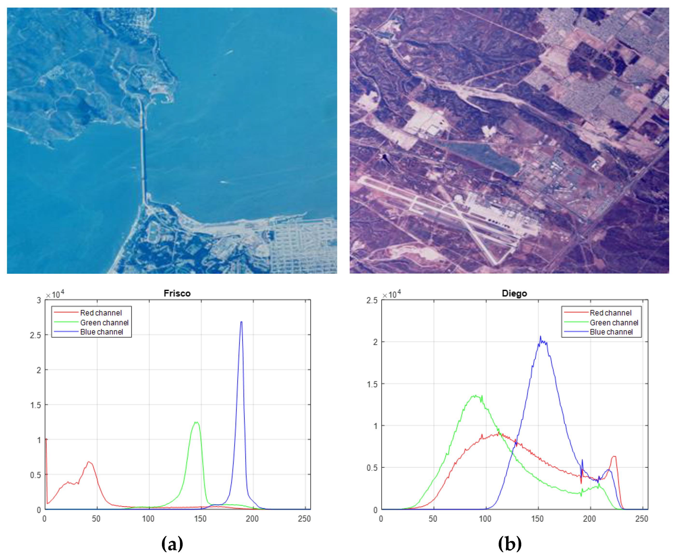
Secondly, the correlation between component images of three-channel RS data can differ from the correlation of red, green, and blue components of color images. Whilst, for color images, the cross-correlation factor is usually around 0.7 [42], the correlation factor between components of three-channel RS data may be significantly higher [5]. This might influence noticeably the final compression performance if 3D approaches are to be applied.
Since individual channels of RGB images are represented as 8-bit data and such components of RS images might be initially represented in another way, e.g., as 16-bit data, it may be difficult to adequately compare the compression of color and three-channel RS images. Therefore, three-channel images with the 8-bit representation of channels (also referred to as component images) are considered in a further part of the paper. Additionally, if component images originally have more than 8 bits, it is supposed that they are pre-normalized to 8 bits before lossy compression. Certainly, this leads to the introduction of some additional errors, although relatively small, due to rounding to the nearest integer. The PSNR of images subject to normalization, rounding-off, and re-normalization is usually around 59 dB, whereas distortions introduced during lossy compression usually lead to a much smaller PSNR. Thus, distortions caused by normalization (if applied) may be ignored in further analysis.
Furthermore, there are no commonly accepted databases of “pristine” (reference, distortion-free) RS images. Moreover, types of distortions inherent for RS images and color images partly coincide but are partly different. For example, image dithering is not met in practice in RS images. Meanwhile, speckle noise is not typical for color images but it might be an important factor for RS images of a special kind (synthetic aperture radar ones). This obstacle prevents the direct use of color image databases for making conclusions and recommendations for RS images. However, recently, the TID2013 dataset has been indirectly used to analyze the subsets of distortion types that might be present in RS images. This has allowed the determination of good elementary visual quality metrics for the adequate characterization of RS image quality and the design of combined metrics. Already known visual quality metrics, used in a combined metric [16] as one of the inputs, are referred to as elementary metrics. In particular, the MDSI [28] has been presented as one of the best elementary metrics [16]. Hence, more details about this metric are provided below, together with an explanation of why it has caught our attention.
It should be kept in mind that the visual quality metrics describe the quality of data from a specific viewpoint and the relation between visual quality metrics and, e.g., text recognition from document images or image classification accuracy is not fully known [29]. Nevertheless, preliminary results of the classification of compressed images have already demonstrated that visual quality has a high correlation with classification accuracy, especially for classes represented by small-sized, prolonged, and textural objects, i.e., for classes that are quite heterogeneous [16]. Since high-frequency information can be lost due to lossy compression for large CR, it might harm the classification as well.
Our task of providing desired quality in compressing a given image can be treated as a particular case of applying the theory of generative adversarial nets [43,44,45] since the image at hand is supposed to belong (according to its basic properties) to the set of images used at the method training stage when the average rate distortion curve has been obtained. Although there are some papers studying how distortions affect image classification and object recognition tasks, particularly with the use of neural networks, it should be kept in mind that lossy compression should not lead to an essential degradation in performance for image classification and object recognition compared to uncompressed original data.

2.2. Analysis of Some Elementary Image Quality Metrics

Image quality assessment (IQA) plays a significant role in numerous image processing applications—for example, image acquisition, lossy compression, restoration, denoising, etc. IQA techniques and metrics can be divided into three categories according to the availability of the original image, namely Full-Reference (FR), Reduced-Reference (RR), and No-Reference (NR). Different methods may be chosen according to the requirements, their priority, and their application. In this paper, the FR IQA methods are utilized to evaluate the compressed images and to provide the desired visual quality in RS lossy compression. The main reason is the knowledge of the reference image (this is simply the image to be compressed). Another reason is that the FR IQA metrics are usually simpler and more adequate (accurate) than the metrics that belong to the two latter groups.
The simplest classical FR IQA metric is the Mean Squared Error (MSE), computed by averaging the squared intensity differences of distorted and reference images pixel-wise. Another well-known metric strictly related to MSE is the Peak Signal-to-Noise Ratio (PSNR). The significant advantages of MSE and PSNR are that their calculation is simple and their physical meaning is clear since the contrasting is based on the pixel level. Nevertheless, the most relevant weakness of these metrics is that they are not very well matched to perceived visual quality [46]. Because of this, numerous metrics based on the MSE and other principles, particularly calculated locally using the sliding window approach, have been proposed and intensively studied in the last three decades, i.a., Structural Similarity (SSIM) [47,48,49], Feature Similarity (FSIM) [50], or the MDSI [28].
In this paper, the MDSI is adopted as the visual quality metric for three-channel RS images. To explain the reasons for this choice, some aspects and requirements for IQA should be recalled. As is widely known, subjective image visual quality is assessed during quite complicated experiments involving a large number of participants and test images of different complexity [38]. The result of such testing consists in obtaining Mean Opinion Score (MOS) or Differential Mean Opinion Score (DMOS) values. A metric is considered good if, for different databases, it has high absolute values of correlation factor between a given metric and MOS, where both conventional (Pearson) and rank-order (Spearman and/or Kendall) correlations can be taken into consideration (ideally, it is desired that both Pearson and Spearman correlation coefficients have absolute values close to unity). As the first requirement, monotonicity of dependence of a metric on image quality characterized by Spearman Rank Order Correlation Coefficient (SROCC) is required. Meanwhile, linearity of this dependence, better characterized by the Pearson Linear Correlation Coefficient (PLCC), is desired as well. Note that the above-mentioned FSIM [50] has sufficiently nonlinear behavior on image quality and MOS [51]. During some experiments conducted for 50 metrics [16], SROCC values have been calculated as one quantitative criterion of metric performance for all distortion types and three subsets of the Tampere Image Database (TID2013). According to these calculations, the SROCC value determined for MDSI versus MOS is 0.8897 for all types and levels of distortions, being higher than for most other metrics, whereas the SROCC for the subset Noise&Actual is 0.9374. It is the highest value among all the considered elementary metrics. Meanwhile, the statistics of average calculation time demonstrate that the computational efficiency of the MDSI is very high. Additionally, the SROCC between MDSI and MOS has been calculated for images with three types of distortions related to lossy compression in the TID2013 dataset. It is equal to 0.966, i.e., very high, meaning that the MDSI is able to adequately characterize the visual quality of lossy compressed images.
Although the detailed SROCC values for 50 elementary metrics obtained for three subsets and the whole TID2013 dataset may be found in the paper [16], an additional verification of these metrics may be conducted for the Konstanz Artificially Distorted Image quality Database (KADID-10k) [52], containing 81 pristine images, each degraded by 25 distortions in five levels—particularly for the subsets containing distortions characteristic for RS images. Considering the JPEG and JPEG2000 compressed images, only two metrics—HaarPSI and MDSI—achieve SROCC values over 0.925 and PLCC over 0.94 (after nonlinear fitting) simultaneously, demonstrating both high prediction monotonicity and accuracy. Nevertheless, it is worth noting that the HaarPSI metric is around 1.4 times slower than MDSI, being one of the fastest elementary metrics (detailed results are presented in the paper [16]). The performance comparison of individual metrics for the lossy compressed images from the KADID-10k dataset is presented in Appendix A (Table A1).

2.3. The MDSI Metric and Its Properties

An important property of the MDSI metric is that, during its computation, a gradient magnitude is used to measure structural distortions, whereas chrominance features are used to measure color distortions (recalling that both these types of distortions are equally important for three-channel RS images). Subsequently, the two obtained similarity maps are combined to form a gradient-chromaticity similarity map. Differently than for SSIM and FSIM, the deviation pooling strategy is used to compute the final quality score. In comparison to previous research, this new gradient similarity map is more likely to follow the human visual system (HVS).
Providing the desired visual quality in lossy compression is a challenging task; however, it would be possible if a metric value was associated with a certain level of quality. It could also be useful to know a range of metric values for which distortions are practically invisible. In lossy compression, the desired visual quality is often within a certain range, also for RS images. As illustrated by some already completed analyses based on other metrics [33], the lower limit is such that lossy compression has no negative impact on further image processing. It means that the introduced distortions may be noticeable or even visible but not annoying. Concerning the upper limit, the lossy compression should provide a higher CR than possible to achieve by the lossless compression (limited by entropy). A reasonable threshold should be set in such a way that the introduced distortions are invisible, so the visual quality of compressed data should be identical to lossless compressed images but higher CR can be achieved. This threshold is around 40 dB in terms of the PSNR-HVS-M metric multi-channel RS images [33].
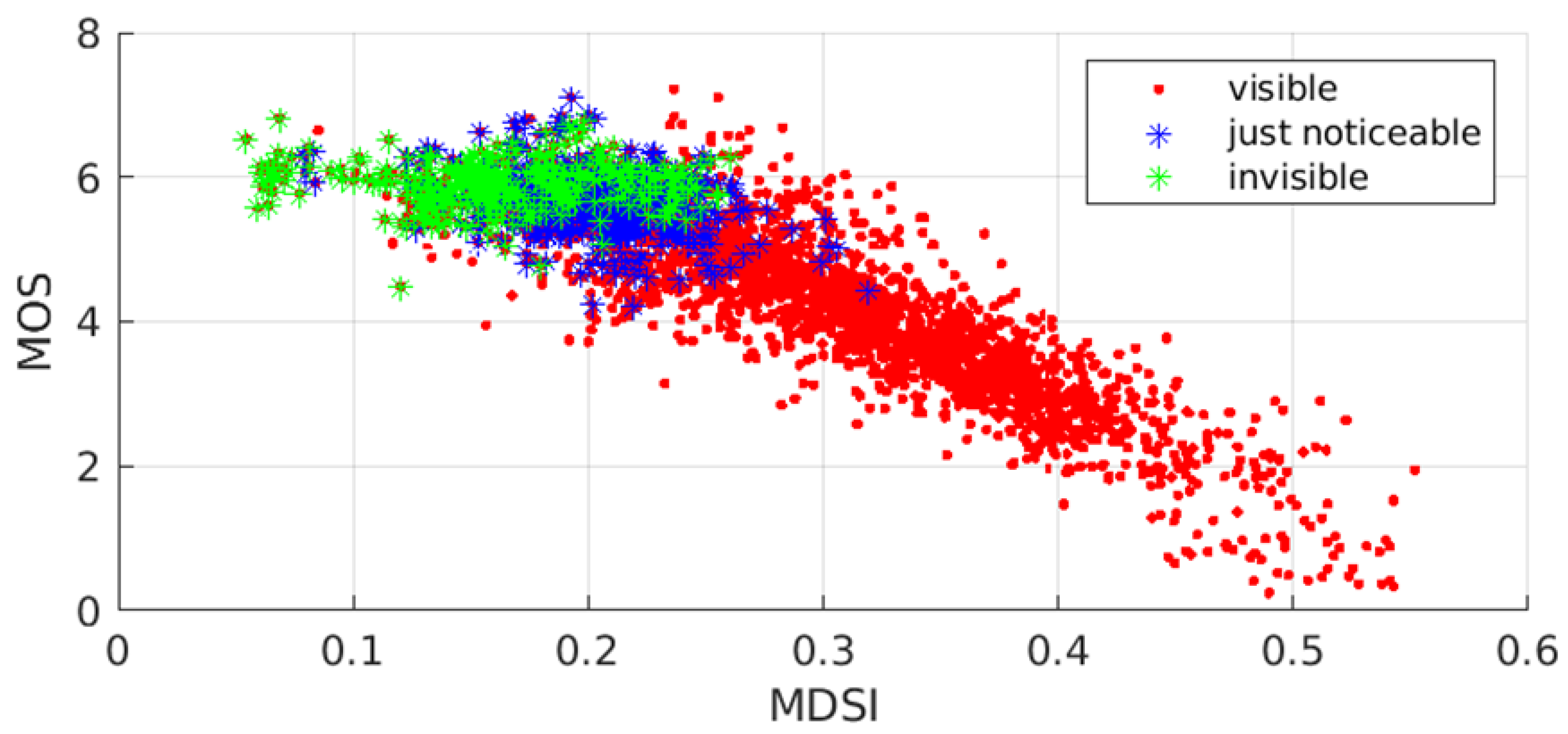
To provide a reasonable range for the metric MDSI, we have tested 3000 color images of the database TID2013 to obtain the statistical data results [38] and put them into three categories, namely visible, just noticeable, and invisible distortions. Since MOS values have been provided for each image in the TID2013 dataset, the scatter plot for MDSI vs. MOS for the three mentioned classes of images is shown in Figure 1.
Combining the statistical results and MOS values, it can be approximately stated that there are three gradations of image quality according to MDSI:
  • excellent quality (MDSI ≤ 0.15), the distortions are mostly invisible;
  • good quality (0.15 < MDSI ≤ 0.25), the distortions can be just noticeable;
  • middle and bad quality (MDSI > 0.25), the distortions are visible or they can be annoying.
Therefore, the reasonable range (under interest in this paper) is set as the range from 0.10 to 0.25. It is also worth noting that the relation between MDSI and MOS is almost linear and this should be considered as one more advantage of the MDSI metric.

3. The Two-Step Method for Lossy Compression

The two-step image compression method has been recently proposed to control the visual quality in lossy compression, and further provide the desired visual quality for handling images in terms of a chosen visual quality metric. The previous research has proven that this method works well for DCT-based coders (such as AGU, ADCTC) [35,53] as well as for the DWT-based coder (SPIHT) [54]. The latest conference paper [36] demonstrates also some initial results and the advantages of the two-step compression method for the BPG coder.
Although lossy compression can easily achieve higher CR than lossless compression, usually, it reduces the visual quality of an image noticeably. However, the visual quality is also important and it can be even the most important requirement in some cases. Consequently, in such applications, lossy compression should be applied with additional control of introduced distortions. To control the visual quality in lossy compression, the CCP can be adjusted (or just properly set), considering the so-called rate-distortion curve, representing the dependence of visual quality on the CCP. However, for a given lossy compression coder, visual quality dependence on the CCP varies, depending also on image characteristics. Although it is difficult to know the rate-distortion curve for each image to be compressed in advance, it is still possible to obtain the general trend for particular image categories, e.g., three-channel RS images.
Since the provided approach should be possible to apply for images of different terrains or, in other words, of different complexity containing various types of objects, a relatively high number of test images should be used in experiments. This requirement is one of the main reasons for the methodology of design and analysis applied at different stages of the study presented in the paper.
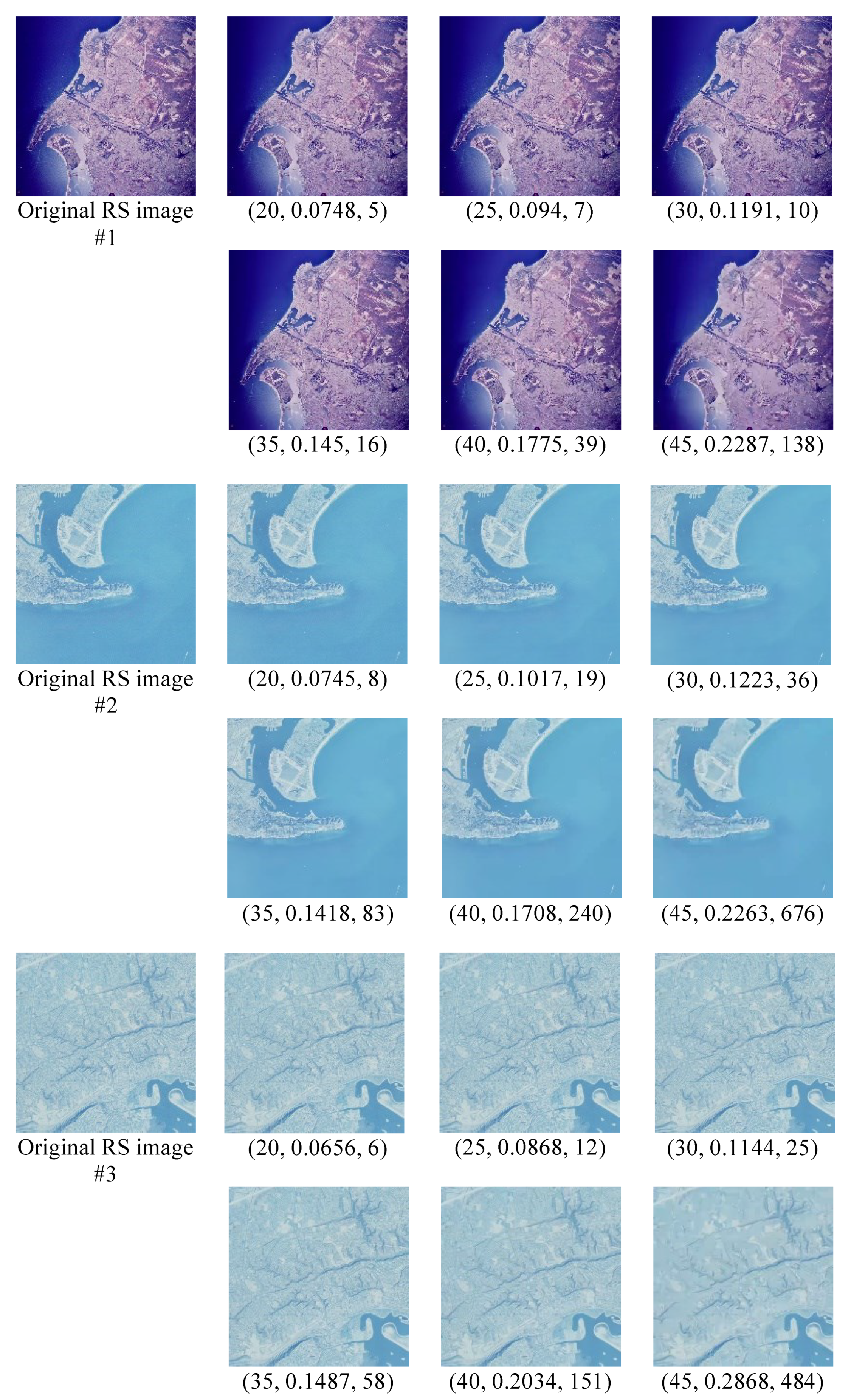
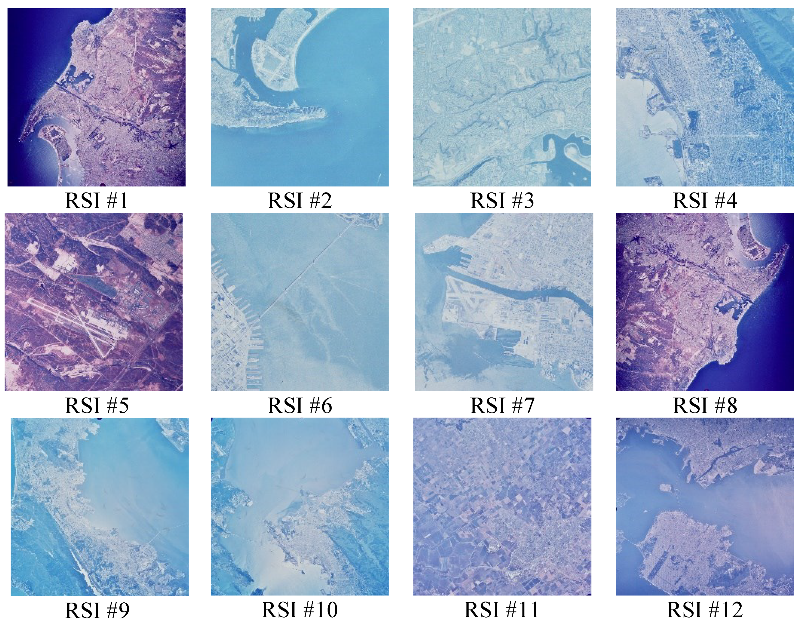
First of all, a certain number of images are chosen to be compressed/decompressed assuming a series of CCP values, further referred to as the basic image set (sample images are shown in Figure 2). Each value of MDSI for each test image obtained after compression/decompression using given 
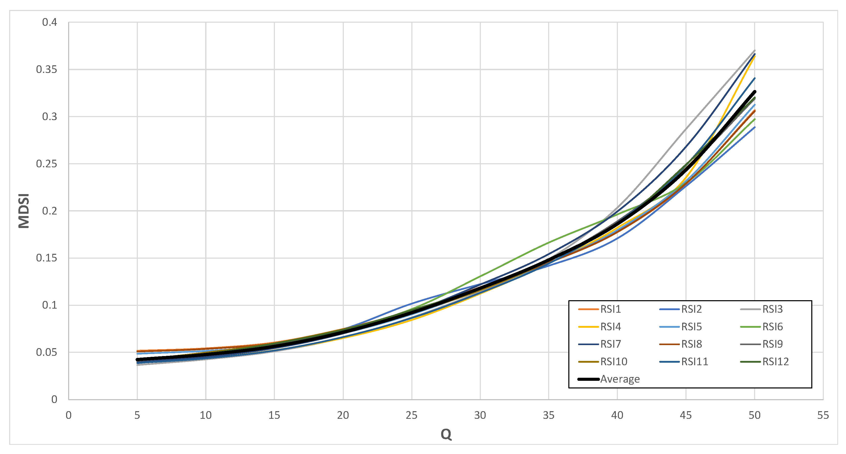
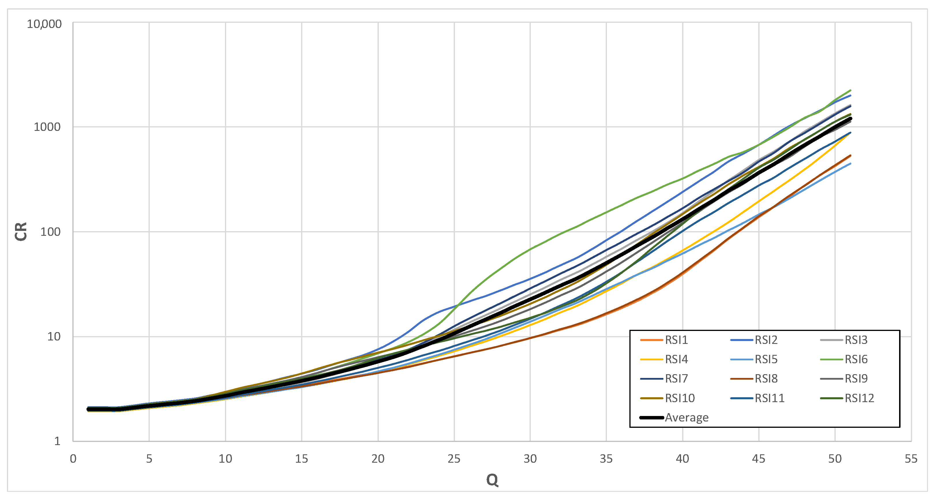
CCP values should be registered to evaluate the distortions. As a consequence, a model of visual quality metric dependence on the CCP may be obtained from these statistic data. At this stage, it is possible to obtain individual dependencies of the metric on the CCP, further averaged for all basic images corresponding to each CCP (more details are provided in Section 4). In this way, it is also possible to obtain an averaged dependence, the so-called average rate-distortion curve, which reflects the monotonous change in visual quality with the CCP. This process is performed offline; hence, it does not influence the time efficiency of the two-step method. Based on this average rate-distortion curve, the second step of the method can be carried out.
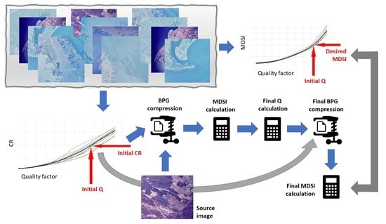
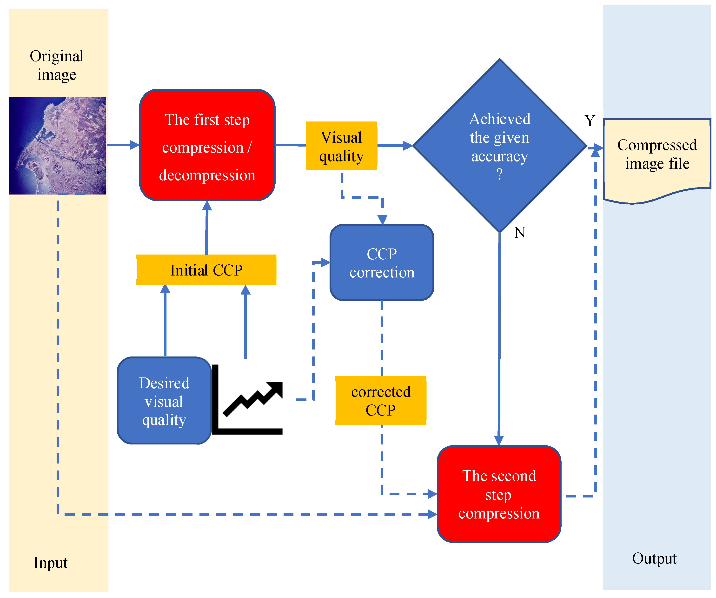
The block diagram of the two-step compression method is illustrated in Figure 3; in the first step, the initial CCP is determined using the desired visual quality and the average rate-distortion curve. In general, it is calculated using the following equation:
C C P i n i t = C C P e s t + M d e s + M a v g M ,
where M d s t is the desired visual quality pre-set by the user, and the other three parameters come from the average rate-distortion curve presented in a tabular form. The M a v g is the value closest to the desired M d e s at the right end of the corresponding interval of the average rate-distortion data array, whereas C C P e s t is the value corresponding to M a v g . The curve derivative for the corresponding C C P e s t is denoted as M . These calculations do not require image compression, so the C C P i n i t value is the same for all images being compressed, assuming a given desired visual quality.
The first step of the proposed method is the compression and decompression of the original image with the initial CCP; subsequently, the visual quality value M i n i t of the decompressed image could be calculated using the original image as the reference. Since the metric value M i n i t is close to the desired M d e s , the absolute error is calculated as
Δ M = M i n i t M d e s ,
further evaluated as acceptable or not to undertake a decision concerning further actions. It is worth noting that, for some images, the above Δ M error can achieve the required level, so the second step is not needed and the compressed image in the first step can be treated as the final output.
To improve the accuracy of provided visual quality, the CCP value needs to be corrected before the second step using the following equation:
C C P d e s = C C P i n i t + M d e s + M i n i t M .
This corrected CCP value may be different for different images. Finally, the second step, compression, is carried out using the C C P d e s , and the compressed image file obtained after the second step is considered as the final output with the desired quality.

4. The Implementation of the Two-Step Method for the BPG Coder

Since the demand for high-quality images with acceptable size has been dramatically increased, there have been numerous conventional lossy compression coders developed [21,31,54,55,56] that may be applied not only for typical three-channel RGB images. One of the most interesting recent concepts is known as the Better Portable Graphics (BPG), which is a novel image compression method that aims to replace the decades-old JPEG format due to considerably better performance in the sense of higher quality and/or lower size [57]. Even though, recently, some learned lossless and lossy image compression methods have been proposed, the BPG is still highly competitive [58]. In this paper, it is utilized as the lossy compression coder applied to compress three-channel RS images. The description of the implementation of the two-step compression method for the BPG coder is provided further.

4.1. The BPG Coder

The BPG coder is based on the High Efficiency Video Coding (HEVC) [59,60] technique, which was proposed by Fabrice Bellard in the form of the open-source code (More details available at: https://bellard.org/bpg/ (accessed on 23 February 2022)). Compared to JPEG, the BPG coder ensures a higher compression ratio for the same quality. Additionally, the BPG has the following important attributes:
  • it provides a JavaScript decoder, increasing the accessibility of the BPG to most web browsers and portable applications due to its lightweight code;
  • it is open-source, royalty-free, and patent-free;
  • it supports the same chroma formats as JPEG (grayscale, YCbCr 4:4:4, 4:2:2, 4:2:0 with the use of Lanczos filters) to reduce the losses during the conversion, as well as an alpha channel, RGB, YCgCo, and CMYK color spaces;
  • it supports natively 8 to 14 bits per channel, although, in most applications, 8 bits are used, similarly as in this paper;
  • it supports lossless and lossy compression.
As mentioned above, the BPG algorithm is an essential part of the HEVC video encoder [59,60], which is treated as a sufficient advance in video compression technology. The high efficiency of HEVC is explained by the intelligent approach to block size and the use of the DCT or the Discrete Sine Transform in the spatial frequency domain.
Regardless of some patent issues of the HEVC implementations (More details available at: https://www.loc.gov/preservation/digital/formats/fdd/fdd000530.shtml (accessed on 30 March 2022)), all the above features make the open-source BPG a highly competitive candidate for the replacement of many existing image compression algorithms. Some details concerning its hardware implementation may be found in the paper [61].
The parameter Q, used internally to control the compression ratio and image quality in the BPG encoder, is considered as the CCP, where Q { 1 , , 51 } and a larger Q results in a higher CR, corresponding to lower visual quality [36]. Unlike the CCP in AGU and SPIHT, the parameter Q takes only integer values. The BPG encoder may also use JPEG or PNG images as input, performing BPG compression, and producing the corresponding BPG image.
The BPG performance has already been compared to many other coders in terms of standard and visual quality metrics [62,63,64]. It has been demonstrated that the BPG outperforms JPEG and JPEG2000 [62]. It also performs approximately at the same level as modern autoencoders based on learning [63,64].
In addition, a special comparison has been carried out for the considered case, i.e., for the MDSI metric and color RS images. Two 512 × 512 pixel color images for simple and complex structures (Frisco and Diego, respectively), shown in Figure 4, have been processed to produce three different values of MDSI: 0.1, 0.15, and 0.2. The analysis of the provided histograms shows the prevailing influence of the blue component in both cases. The same holds, in general, for other three-channel images used in our studies.
The CR values have been obtained for the BPG (version 4:2:2), the 3D version of the AGU coder [65], JPEG, and JPEG2000 [66]. The data are collected in Table 1. Their analysis shows that the BPG slightly outperforms the 3D AGU and JPEG2000 for the middle values of the Q parameter (high quality of compressed images) and has obvious benefits for large Q values (low quality of the compressed image). Additional data on the comparison of coders can be found in [32,33], showing that better performance of a coder usually leads to better classification.

4.2. Calculation of the Average Rate-Distortion Curve According to the MDSI

The prime task in the implementation of the two-step method for the BPG coder is to obtain the average rate-distortion curve for the considered visual quality metric (MDSI). Based on the analysis provided in Section 3, this average rate-distortion curve results from statistical data from a certain number of images. In this paper, twelve 1024 × 1024 pixel three-channel RS images taken from the USC-SIPI dataset (volume 2: Aerials) (The USC-SIPI image database is available at: http://sipi.usc.edu/database/database.php?volume=aerials (accessed on 23 February 2022)) have been chosen as the basic image set, shown in Figure 5. Then, the compression and decompression have been carried out for each image with various CCP values, where all possible values of the Q parameter have been used.
To obtain the average rate-distortion curve, MDSI values have been calculated for all 612 images (12 original images and 51 values of the Q parameter), and further averaged for the individual Q values. The obtained curves are presented in Figure 6 independently for each of the images used in the experiments. The obtained curves may be divided into four areas for further analysis:
  • Q 3 —the visual quality is constant and very high;
  • 4 Q 25 —the visual quality starts to change slowly, and the MDSI values for different images are very similar;
  • 26 Q 40 —the visual quality changes more significantly, but the deviations between quality indicators of different images are still small;
  • Q 41 —the visual quality starts to rapidly decline and the deviations of the MDSI values for different images become obvious.
Consequently, the optimal work area of the Q parameter seems to be [26, 40], and the corresponding range of the MDSI values is [0.1, 0.25].
The two-step compression can be carried out for the BPG using the average rate-distortion curve (shown in Figure 6), but the implementation differs from the previous scheme. Formula (1) is not needed and the Q i n i t may be set as the nearest integer Q producing the desired MDSI value according to the average rate-distortion curve. In other words, Q i n i t equals Q e s t . Additionally, since the value of Q after the correction according to Equation (3) is, most probably, non-integer, a rounding-off operation is needed for the Q. More detailed experimental results obtained for the basic image set are provided in Appendix A (Table A2).
Since the curves in Figure 6 partly overlap, the MDSI values obtained for ten values of the Q parameter for the considered test images are also presented in Table 2. Whilst the MDSI values are almost the same for small Q values (where the introduced distortions are anyway invisible), sufficient differences can be observed for large Q (e.g., data for Q equal to 40 and 45, which are of practical interest).
To obtain an initial insight about the CR and its variation depending on image properties, Figure 7 illustrates the corresponding data. Whilst the CR values are small and do not vary significantly for small Q values, they are quite large (significantly larger than for lossless compression) and vary strongly for the Q values starting from 20. This explains our special interest in the Q values within the limits from around 20 to approximately 45, corresponding to MDSI values from around 0.07 to 0.28.
The pseudo-code illustrating the main idea of the method is provided in Algorithm 1.
Algorithm 1 Quality control algorithm flow.
Require: original image, desired MDSI value, Q array, MDSI average array, derivative array
  1: for i = 1 to 50 do
  2:     repeat
  3:         Calculate mean(MDSI[i]) − desired MDSI
  4:         i++
  5:     until mean(MDSI[i]) − desired MDSI > 0
  6: end for
  7: Calculate the initial Q
  8: Perform the BPG compression according to initial Q
  9: Record the initial MDSI 10: Calculate the final Q
11: Round up Q
12: if final Q = initial Q then
13:     return initial MDSI
14: else
15:     Perform the BPG compression according to the final Q
16:     return final MDSI
17: end if

5. The Experimental Results

To evaluate the performance of the proposed two-step method for the BPG coder for three-channel RS images, some additional test experiments are necessary since the average rate-distortion curve model has been obtained only for the basic image set, which might be not representative enough. Consequently, the two-step compression method has been applied firstly for the basic image set to provide four typical values for the MDSI metric, representing the four classes provided in Section 4.2. These four typical values have been set as 0.1, 0.15, 0.2, and 0.25, respectively, and the achieved statistical data are shown in Table 3, where M d e s denotes the desired value of the MDSI metric, V A R 1 stands for the variance of MDSI provided in the first step, and V A R 2 is the variance of MDSI provided in the second step. For a better understanding of the data, the mean MDSI values finally provided in the second step are provided as well, denoted as M E A N 2 .
The analysis of the data provided in Table 3 leads to the conclusion that the variance after the second step of compression has decreased by approximately one order of magnitude for each desired value. It proves that the proposed two-step procedure works well in the considered conditions. It can also be noticed that both variances V A R 1 and V A R 2 tend to increase if the desired MDSI increases. This means that the task of providing the desired MDSI is more important for larger M d e s values, e.g., 0.2 or 0.25 (for M d e s = 0.1, the distortions are invisible and they remain invisible if the desired MDSI is provided with the error of around 0.01).
The mean absolute error of the desired quality, calculated as M d e s M E A N 2 , does not exceed 0.034, and its value increases as the desired visual quality decreases, which is similar to the trend observed in previous works with the other coders [35,54].
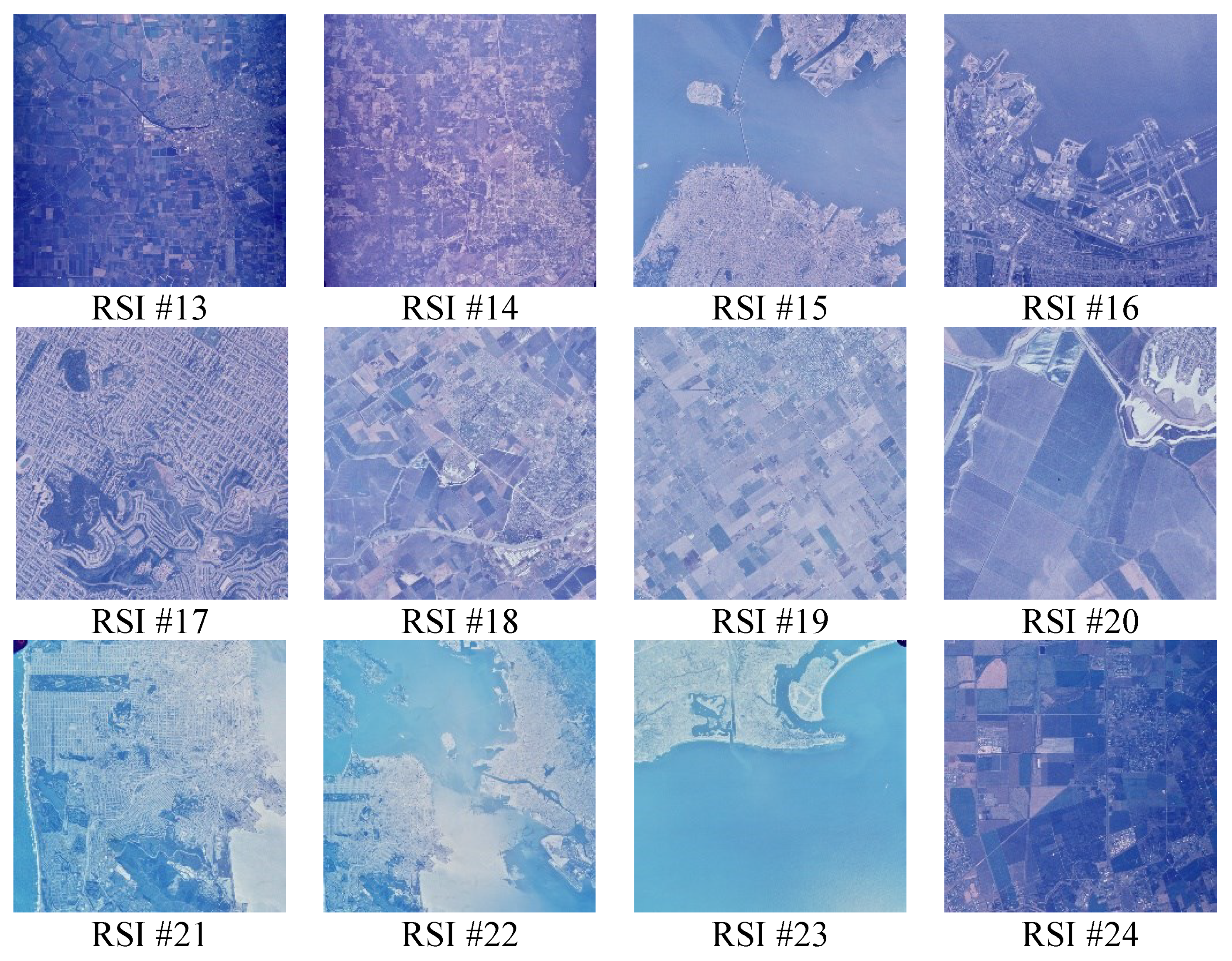
To verify the representativeness of the basic set, the other 12 RS images have been chosen as the test image set, shown in Figure 8 (further referred to as RSI #13–#24), which is also a part of the USC-SIPI dataset. Then, the two-step compression method has been applied to these images to verify the correctness and universality of the previously obtained curve model, leading to the statistical data shown in Table 4.
As shown in Table 4, for each desired MDSI value, the variance after the second step of compression has also decreased by approximately an order of magnitude, and the mean error does not exceed 0.035. As one can see, the tendencies and values are similar to those observed in Table 3, so the basic image set has been chosen correctly to obtain the average rate-distortion curve and this model works well for other three-channel RS images.
To analyze the data for 12 test images (RSI #13–#24) in detail, results obtained for M d e s = 0.25 are presented in Table 5, where Q i n i t denotes the parameter Q used for the first step of compression. It comes from the average rate-distortion curve and equals 45 for all images. As may be seen in Table 5, although the initial MDSI values are different for individual test images, their variance after the second step has decreased significantly, being only 1/15 of its value after the first step. The mean value of the MDSI after the second step is also noticeably closer to 0.25; hence, its average relative error has also decreased (from 2.08% to 1.4%).
In general, the accuracy has radically improved due to the second step of compression. Meanwhile, there are cases when the MDSI after the second step is the same as for the first step, e.g., this happens for RSI #13. This means that there is no need to correct the Q parameter and apply the second step of compression in such cases. As shown in Table 5, 5 out of 12 images needed only one-step compression to meet the quality requirements, whilst the other seven images needed the second step to improve the accuracy. For all verification experiments (carried out for all 24 images and four desired MDSI values), 28.1% of images needed only the first step of the two-step compression to provide the desired visual quality. The other tables with more detailed results, both for the basic and the test image sets, achieved for different desired MDSI values, are provided in Appendix A (Table A3, Table A4, Table A5, Table A6, Table A7, Table A8 and Table A9).

6. Discussion

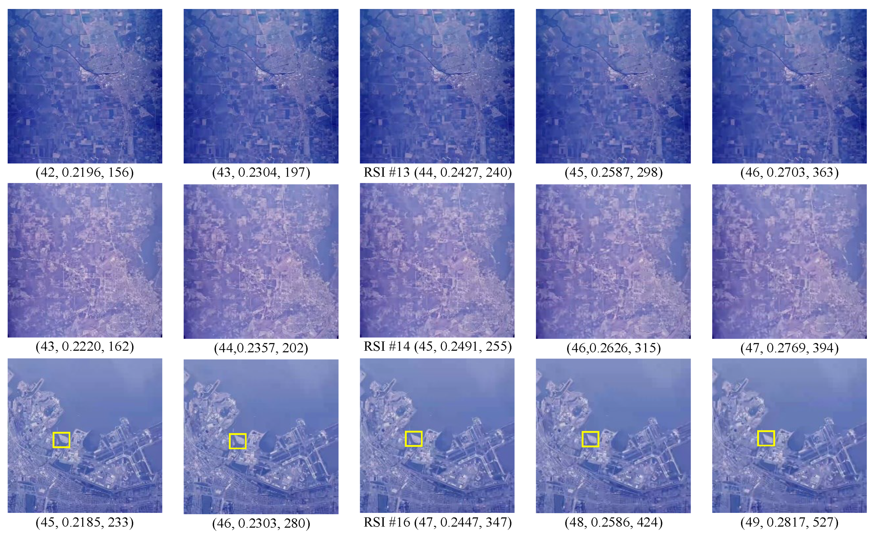
To analyze the accuracy of the provided visual quality for the BPG-based lossy compression of three-channel remote sensing images, three images (RSI #13, #14, and #16) have been selected as representative examples with the desired visual quality (MDSI) equal to 0.25.
The decompressed images for the two-step compression method are shown in the middle (third) column in Figure 9. For the desired MDSI value equal to 0.25, the initial Q is equal to 45; the calculated Q d e s values are different for different images (equal to 44, 45, and 47, respectively). The two images on the left from the third column are the images obtained if the parameter Q is set as Q d e s 1 and Q d e s 2 , and the two images on the right are the images when Q is set as Q d e s + 1 and Q d e s + 2 .
For RSI #14, Q i n i t appears to be the appropriate value as for its change (increase or decrease), the error Δ M D S I = M D S I f i n a l M D S I d e s increases. For RSI #13, the parameter Q is corrected to 44, and in comparison to the four other values, compression with the Q d e s produces M D S I f i n a l , which is the closest to the M D S I d e s . In contrast, for RSI #16, the initial Q is corrected to 47, and compression with this Q d e s produces the smallest error between M D S I f i n a l and M D S I d e s . Concerning the error, for RSI #16 considered as an example, the provided M D S I f i n a l is 0.2447, and the error between M D S I f i n a l and M D S I d e s is 0.0053. Figure 9 shows five decompressed images resulting from RSI #16, where images compressed with two values of Q differing by unity seem to be practically identical, but if Q differs by 2 or more, e.g., for RSI #16 (45, 0.2185, 233) and RSI #16 (49, 0.2817, 527) compared to RSI #16 (47, 0.2447, 347), the difference is much easier to observe. Hence, if the difference Δ M D S I is approximately 0.015, it is difficult to observe the changes in the decompressed images. However, it becomes noticeable if Δ M D S I is approximately 0.03, e.g., for RSI #16 (46, 0.2303, 280) and RSI #16 (48, 0.2586, 424). Therefore, in practical applications, it is enough to ensure errors of providing the desired MDSI less than ≈0.01. Consequently, it can be drawn that the accuracy of the two-step method for the BPG coder is good enough.
In summary, for images where the second step is necessary, regardless of whether the correction is forward or reverse (initial Q is increased or decreased), it gives a positive impact and eventually provides the visual quality that is the closest to the desired one. Additionally, the CR values provided for image lossy compression in the neighborhood of the distortion invisibility threshold are considerably higher than possible to achieve using a lossless compression.
To analyze the computational efficiency of the proposed approach, some tests have also been performed using a notebook with an Intel® Core™ i7-4710HQ CPU @2.50 GHz and 16.0 GB RAM, controlled by the 64-bit Windows 10 Pro operating system for the x64 processor architecture. For 512 × 512 pixel images, the compression time is from 0.02 s to 0.05 s depending on image complexity and the value of the parameter Q (a larger time is needed for more complex structure images). The decompression time is from 0.006 s to 0.019 s (more time is spent on the decompression of more complex structure images). For 1024 × 1024 pixel images, the compression time is from 0.06 s to 0.12 s; the decompression time is sufficiently smaller (from 0.02 s to 0.06 s). The MDSI values can be calculated very quickly (the time for their calculation is only around 1.5 times longer than for the calculation of MSE).

7. Conclusions

In this paper, a two-step algorithm for providing the desired visual quality for the BPG-based lossy compression of three-channel remote sensing images has been proposed. The MDSI metric has been applied to evaluate the visual quality of the decompressed image. The main contributions of this paper concern the extensions of the basic two-step algorithm utilizing the MDSI metric and some features of the BPG encoder, e.g., integer form of the Q parameter, as well as the properties of three-channel RS images, such as high correlation of multi-channel data.
The MDSI metric has been studied to evaluate the quality of three-channel images, providing a reasonable operation range for the lossy compression of three-channel RS images. Three visual quality levels have been proposed, corresponding to the MDSI values appropriate for excellent quality, good quality, as well as middle and bad quality, respectively.
Experimental results have demonstrated the superiority of the proposed algorithm. It allows images to be compressed quickly and with appropriate errors concerning the desired quality characterized by the MDSI metric. If the parameter Q, calculated after the second step, is equal to the initial Q, the second step could be skipped and the procedure may be accelerated for some similar images or video frames. Otherwise, the second step is needed to improve the accuracy with the corrected Q value. Statistical data show that, due to the second step, the accuracy is considerably improved and the provided visual quality is very close to the desired one. Our methodology is quite general and can also be applied to some other metrics having similar performance to MDSI.
In the future, it is expected that BPG-based lossy compression can be applied to provide the desired characteristics of the classification of decompressed images. A study concerning the impact of visual quality evaluated by the MDSI on the accuracy of classification is planned, as well as a discussion of the applicability of the two-step algorithm for the BPG coder in the classification task of high-resolution multi-channel remote sensing images.

Author Contributions

Conceptualization, F.L. and V.L.; methodology, F.L., O.I. and V.L.; software, F.L. and O.I.; validation, V.L. and K.O.; formal analysis, V.L. and K.O.; investigation, F.L., O.I., V.L. and K.O.; resources, F.L., O.I. and V.L.; data curation, F.L., O.I. and V.L.; writing—original draft preparation, F.L., V.L. and K.O.; writing—review and editing, V.L. and K.O.; visualization, F.L. and O.I.; supervision, V.L.; project administration, V.L. and K.O.; funding acquisition, F.L., V.L. and K.O. All authors have read and agreed to the published version of the manuscript.

Funding

The research is partially co-financed by the Polish National Agency for Academic Exchange (NAWA) and the Ministry of Education and Science of Ukraine under the project no. PPN/BUA/2019/1/00074 entitled “Methods of intelligent image and video processing based on visual quality metrics for emerging applications”. The support provided to Fangfang Li during her studies at the National Aerospace University by the China Scholarship Council (CSC) is also acknowledged.

Institutional Review Board Statement

Not applicable.

Informed Consent Statement

Not applicable.

Data Availability Statement

Not applicable.

Conflicts of Interest

The authors declare no conflict of interest. The funders had no role in the design of the study; in the collection, analyses, or interpretation of data; in the writing of the manuscript, or in the decision to publish the results.

Abbreviations

BPGBetter Portable Graphics
bppbits per pixel
CCPcompression controlling parameter
CRcompression ratio
DCTDiscrete Cosine Transform
DMOSDifferential Mean Opinion Score
DWTDiscrete Wavelet Transform
FR IQAFull-Reference Image Quality Assessment
FSIMFeature SIMilarity
HEVCHigh Efficiency Video Coding
HVSHuman Visual System
JPEGJoint Photographic Experts Group
KADIDKonstanz Artificially Distorted Image quality Database
MDSIMean Deviation Similarity Index
MOSMean Opinion Score
MSEMean Squared Error
NR IQANo-Reference Image Quality Assessment
PLCCPearson Linear Correlation Coefficient
PNGPortable Network Graphics
PSNRPeak Signal-to-Noise Ratio
RR IQAReduced-Reference Image Quality Assessment
QSquantization step
RSIremote sensing image
SPIHTSet Partitioning In Hierarchical Trees
SROCCSpearman Rank Order Correlation Coefficient
SSIMStructural SIMilarity
TIDTampere Image Database
USC-SIPIUniversity of Southern California, Signal and Image Processing Institute

Appendix A

The tables provided in the Appendix A contain the performance of the selected elementary metrics for KADID-10k dataset (Table A1), experimental results obtained for the basic image set (Table A2) as well as the results achieved for various desired MDSI values.
Table A1. Performance of selected elementary metrics for the KADID-10k subsets containing compression-related distortions. Metrics are ordered in descending order according to the PLCC values for both subsets obtained after nonlinear fitting.
DistortionsJPEGJPEG2000Both
MetricSROCCPLCCSROCCPLCCSROCCPLCC
IQM2 0.9412 0.9598 0.8774 0.9653 0.9222 0.9602
HaarPSI 0.9472 0.9585 0.8965 0.9681 0.9358 0.9581
RVSIM 0.9419 0.9527 0.8777 0.9637 0.9230 0.9507
ADM 0.9528 0.9692 0.8984 0.9654 0.9384 0.9494
MDSI 0.9405 0.9246 0.8948 0.9619 0.9267 0.9432
VIF 0.9514 0.9327 0.8878 0.9705 0.9249 0.9404
MCSD 0.9447 0.9247 0.9027 0.9535 0.9323 0.9356
CVSSI 0.9438 0.9249 0.8849 0.9402 0.9249 0.9319
DSS 0.9488 0.9141 0.8969 0.9615 0.9291 0.9298
IGM 0.9385 0.9179 0.8688 0.9523 0.9160 0.9256
RFSIM 0.9219 0.9254 0.8446 0.9261 0.9014 0.9228
FSIMc 0.9510 0.9078 0.9119 0.9323 0.9379 0.9200
NQM 0.9175 0.9167 0.8524 0.9264 0.8876 0.9190
PSNRHVSM 0.9354 0.9016 0.8739 0.9591 0.8941 0.9166
PSNRHMAy 0.9338 0.9008 0.8699 0.9584 0.8916 0.9153
FSIM 0.9509 0.9016 0.9018 0.9283 0.9313 0.9136
PSIM 0.9367 0.8969 0.8957 0.9398 0.9250 0.9119
SRSIM 0.9509 0.9076 0.8991 0.9210 0.9297 0.9090
SFF 0.9466 0.9100 0.8864 0.9073 0.9252 0.9068
WSNR 0.9150 0.8921 0.8291 0.9360 0.8807 0.9060
VSI 0.9395 0.8817 0.8865 0.9218 0.9311 0.9021
VIFP 0.9330 0.9060 0.8303 0.9019 0.9048 0.8908
ADD_GSIM 0.9353 0.8850 0.8952 0.8908 0.9281 0.8866
GSM 0.9349 0.8567 0.8497 0.9198 0.9120 0.8836
VSNR 0.9312 0.8884 0.8409 0.9018 0.9034 0.8831
CSSIM 0.9410 0.8484 0.8849 0.9180 0.9265 0.8814
PSNRHVS 0.9168 0.8719 0.8186 0.9174 0.8841 0.8792
PSNRHAy 0.9155 0.8709 0.8161 0.9156 0.8819 0.8772
IWSSIM 0.9489 0.8896 0.8874 0.9096 0.9290 0.8769
ESSIM 0.9328 0.8321 0.8623 0.9181 0.9159 0.8728
PSNRHMA 0.9308 0.8907 0.8075 0.9077 0.8961 0.8675
MSSIM 0.9334 0.8428 0.8740 0.9071 0.9169 0.8583
SSIM 0.9282 0.8531 0.8644 0.9060 0.9056 0.8559
PSNRHMA_mod 0.9134 0.8694 0.7953 0.8863 0.8812 0.8558
PSNRHA 0.9113 0.8591 0.7917 0.8799 0.8782 0.8446
SSIM4 0.9391 0.8395 0.8848 0.9063 0.9095 0.8380
ADD_SSIM 0.9294 0.8447 0.8690 0.8712 0.9110 0.8350
CSSIM4 0.9453 0.8171 0.8892 0.8551 0.9317 0.8228
IFC 0.8640 0.8278 0.8155 0.8085 0.8432 0.8161
UQI 0.7853 0.8251 0.7623 0.7995 0.7786 0.8123
PSNR 0.8837 0.8256 0.6793 0.7131 0.8091 0.7534
MSE 0.8837 0.7443 0.6793 0.6584 0.8091 0.6897
QILV 0.9414 0.8460 0.8500 0.8407 0.9022 0.6656
DSI 0.9197 0.6218 0.8338 0.6826 0.8943 0.5623
CWSSIM 0.9057 0.6002 0.8457 0.4213 0.8911 0.3937
WASH 0.8712 0.8450 0.3685 0.3668 0.2194 0.2765
MSVD 0.2799 0.2824 0.2280 0.1938 0.2314 0.2267
Table A2. The experimental data obtained for the basic image set.
Q MDSI Values for Individual RS Images
#1#2#3#4#5#6#7#8#9#10#11#12AVG
1 0.0517 0.0384 0.0362 0.0391 0.0484 0.0395 0.0398 0.0509 0.0409 0.0417 0.0385 0.0426 0.0423
2 0.0517 0.0384 0.0362 0.0391 0.0484 0.0395 0.0398 0.0509 0.0409 0.0417 0.0385 0.0426 0.0423
3 0.0517 0.0384 0.0362 0.0391 0.0484 0.0395 0.0398 0.0509 0.0409 0.0417 0.0385 0.0426 0.0423
4 0.0517 0.0385 0.0364 0.0392 0.0485 0.0396 0.0398 0.0509 0.0411 0.0419 0.0386 0.0427 0.0424
5 0.0517 0.0386 0.0365 0.0393 0.0485 0.0396 0.0399 0.0509 0.0411 0.0419 0.0387 0.0427 0.0425
6 0.0519 0.0387 0.0369 0.0394 0.0486 0.0399 0.0401 0.0510 0.0413 0.0421 0.0388 0.0428 0.0426
7 0.0520 0.0392 0.0375 0.0398 0.0489 0.0402 0.0405 0.0512 0.0417 0.0425 0.0393 0.0432 0.0430
8 0.0527 0.0410 0.0393 0.0410 0.0498 0.0420 0.0420 0.0520 0.0429 0.0437 0.0407 0.0445 0.0443
9 0.0536 0.0436 0.0411 0.0423 0.0507 0.0439 0.0437 0.0528 0.0454 0.0464 0.0425 0.0464 0.0460
10 0.0543 0.0455 0.0426 0.0436 0.0516 0.0456 0.0452 0.0536 0.0478 0.0498 0.0436 0.0488 0.0477
11 0.0553 0.0476 0.0443 0.0452 0.0524 0.0474 0.0469 0.0546 0.0506 0.0520 0.0452 0.0507 0.0494
12 0.0563 0.0501 0.0460 0.0467 0.0534 0.0492 0.0485 0.0555 0.0526 0.0540 0.0467 0.0531 0.0510
13 0.0573 0.0525 0.0473 0.0483 0.0545 0.0512 0.0504 0.0567 0.0546 0.0561 0.0485 0.0553 0.0527
14 0.0586 0.0552 0.0493 0.0501 0.0556 0.0531 0.0523 0.0581 0.0562 0.0578 0.0501 0.0574 0.0545
15 0.0604 0.0583 0.0511 0.0522 0.0570 0.0553 0.0544 0.0597 0.0583 0.0597 0.0520 0.0593 0.0565
16 0.0622 0.0615 0.0534 0.0541 0.0587 0.0578 0.0571 0.0616 0.0608 0.0623 0.0541 0.0611 0.0587
17 0.0648 0.0645 0.0561 0.0569 0.0610 0.0616 0.0604 0.0643 0.0637 0.0647 0.0569 0.0640 0.0616
18 0.0679 0.0677 0.0591 0.0589 0.0633 0.0654 0.0634 0.0672 0.0662 0.0677 0.0596 0.0668 0.0644
19 0.0720 0.0706 0.0625 0.0621 0.0671 0.0698 0.0666 0.0705 0.0695 0.0709 0.0632 0.0700 0.0679
20 0.0748 0.0745 0.0656 0.0651 0.0703 0.0735 0.0701 0.0741 0.0729 0.0746 0.0663 0.0740 0.0713
21 0.0781 0.0781 0.0689 0.0680 0.0734 0.0770 0.0735 0.0771 0.0762 0.0776 0.0698 0.0776 0.0746
22 0.0817 0.0833 0.0733 0.0720 0.0773 0.0810 0.0776 0.0811 0.0792 0.0809 0.0734 0.0821 0.0786
23 0.0853 0.0898 0.0776 0.0758 0.0813 0.0854 0.0819 0.0848 0.0835 0.0843 0.0776 0.0859 0.0828
24 0.0898 0.0963 0.0820 0.0803 0.0856 0.0901 0.0869 0.0899 0.0877 0.0880 0.0819 0.0903 0.0874
25 0.0940 0.1017 0.0868 0.0843 0.0904 0.0958 0.0925 0.0944 0.0917 0.0926 0.0864 0.0947 0.0921
26 0.0991 0.1065 0.0922 0.0899 0.0953 0.1022 0.0980 0.0991 0.0956 0.0966 0.0914 0.0996 0.0971
27 0.1035 0.1110 0.0971 0.0950 0.1000 0.1078 0.1039 0.1037 0.1000 0.1014 0.0965 0.1038 0.1020
28 0.1086 0.1151 0.1026 0.1006 0.1060 0.1159 0.1089 0.1083 0.1050 0.1058 0.1015 0.1082 0.1072
29 0.1137 0.1179 0.1087 0.1065 0.1114 0.1234 0.1156 0.1134 0.1104 0.1105 0.1080 0.1129 0.1127
30 0.1191 0.1223 0.1144 0.1122 0.1166 0.1305 0.1218 0.1178 0.1160 0.1158 0.1131 0.1176 0.1181
31 0.1240 0.1263 0.1204 0.1183 0.1227 0.1375 0.1279 0.1234 0.1218 0.1221 0.1188 0.1236 0.1239
32 0.1300 0.1303 0.1266 0.1247 0.1281 0.1453 0.1346 0.1290 0.1279 0.1282 0.1253 0.1293 0.1299
33 0.1332 0.1334 0.1337 0.1305 0.1322 0.1520 0.1402 0.1332 0.1328 0.1339 0.1309 0.1343 0.1350
34 0.1396 0.1369 0.1407 0.1368 0.1380 0.1587 0.1477 0.1387 0.1401 0.1405 0.1374 0.1402 0.1413
35 0.1450 0.1418 0.1487 0.1444 0.1447 0.1664 0.1543 0.1451 0.1469 0.1470 0.1443 0.1477 0.1480
36 0.1518 0.1452 0.1581 0.1513 0.1523 0.1721 0.1622 0.1511 0.1545 0.1555 0.1527 0.1541 0.1551
37 0.1580 0.1505 0.1674 0.1584 0.1590 0.1790 0.1701 0.1578 0.1641 0.1623 0.1607 0.1617 0.1624
38 0.1640 0.1565 0.1777 0.1656 0.1650 0.1856 0.1798 0.1635 0.1715 0.1710 0.1684 0.1697 0.1699
39 0.1710 0.1641 0.1894 0.1737 0.1725 0.1905 0.1883 0.1714 0.1797 0.1789 0.1783 0.1779 0.1780
40 0.1775 0.1708 0.2034 0.1822 0.1797 0.1963 0.1995 0.1777 0.1891 0.1869 0.1876 0.1857 0.1864
41 0.1872 0.1779 0.2177 0.1911 0.1887 0.2024 0.2108 0.1872 0.2011 0.1971 0.1983 0.1966 0.1963
42 0.1956 0.1872 0.2323 0.2008 0.1971 0.2100 0.2209 0.1945 0.2103 0.2087 0.2096 0.2089 0.2063
43 0.2054 0.2013 0.2502 0.2088 0.2080 0.2165 0.2333 0.2057 0.2211 0.2188 0.2214 0.2220 0.2177
44 0.2178 0.2117 0.2712 0.2229 0.2170 0.2230 0.2477 0.2158 0.2319 0.2347 0.2336 0.2388 0.2305
45 0.2287 0.2263 0.2868 0.2354 0.2316 0.2298 0.2680 0.2291 0.2451 0.2454 0.2484 0.2491 0.2436
46 0.2423 0.2384 0.3051 0.2513 0.2454 0.2383 0.2872 0.2428 0.2618 0.2599 0.2625 0.2659 0.2584
47 0.2587 0.2537 0.3209 0.2689 0.2579 0.2499 0.3101 0.2560 0.2721 0.2774 0.2807 0.2784 0.2737
48 0.2743 0.2614 0.3374 0.2965 0.2792 0.2622 0.3259 0.2726 0.2892 0.2924 0.2967 0.2950 0.2902
49 0.2912 0.2707 0.3555 0.3228 0.2933 0.2769 0.3452 0.2855 0.3050 0.3098 0.3190 0.3074 0.3068
50 0.3068 0.2887 0.3701 0.3639 0.3127 0.2973 0.3663 0.3057 0.3190 0.3269 0.3407 0.3203 0.3265
51 0.3281 0.2979 0.3813 0.3949 0.3288 0.3070 0.3770 0.3206 0.3331 0.3389 0.3600 0.3336 0.3418
Table A3. The experimental data obtained for the basic image set for the desired MDSI = 0.1.
Test Image Q i n i t M D S I i n i t Q d e s M D S I f i n a l
RSI #125 0.0940 26 0.0991
RSI #225 0.1017 25 0.1017
RSI #325 0.0868 28 0.1026
RSI #425 0.0843 28 0.1006
RSI #525 0.0904 27 0.1000
RSI #625 0.0958 26 0.1022
RSI #725 0.0925 27 0.1039
RSI #825 0.0944 26 0.0991
RSI #925 0.0917 27 0.1000
RSI #1025 0.0926 27 0.1014
RSI #1125 0.0864 28 0.1015
RSI #1225 0.0947 26 0.0996
VAR 2.24 × 10 5 2.24 × 10 6
MEAN 0.0921 0.1010
Table A4. The experimental data obtained for the basic image set for the desired MDSI = 0.15.
Test Image Q i n i t M D S I i n i t Q d e s M D S I f i n a l
RSI #135 0.1450 36 0.1518
RSI #235 0.1418 36 0.1452
RSI #335 0.1487 35 0.1487
RSI #435 0.1444 36 0.1513
RSI #535 0.1447 36 0.1523
RSI #635 0.1664 33 0.1520
RSI #735 0.1543 34 0.1477
RSI #835 0.1451 36 0.1511
RSI #935 0.1469 35 0.1469
RSI #1035 0.1470 35 0.1470
RSI #1135 0.1443 36 0.1527
RSI #1235 0.1477 35 0.1477
VAR 4.31 × 10 5 6.73 × 10 6
MEAN 0.1480 0.1495
Table A5. The experimental data obtained for the basic image set for the desired MDSI = 0.2.
Test Image Q i n i t M D S I i n i t Q d e s M D S I f i n a l
RSI #141 0.1872 42 0.1956
RSI #241 0.1779 43 0.2013
RSI #341 0.2177 39 0.1894
RSI #441 0.1910 42 0.2008
RSI #541 0.1887 42 0.1971
RSI #641 0.2024 41 0.2024
RSI #741 0.2108 40 0.1995
RSI #841 0.1872 42 0.1945
RSI #941 0.2011 41 0.2011
RSI #1041 0.1971 41 0.1971
RSI #1141 0.1983 41 0.1983
RSI #1241 0.1966 41 0.1966
VAR 1.20 × 10 4 1.32 × 10 5
MEAN 0.1963 0.1978
Table A6. The experimental data obtained for the basic image set for the desired MDSI = 0.25.
Test Image Q i n i t M D S I i n i t Q d e s M D S I f i n a l
RSI #145 0.2287 46 0.2423
RSI #245 0.2263 47 0.2537
RSI #345 0.2868 43 0.2502
RSI #445 0.2353 46 0.2513
RSI #545 0.2316 46 0.2454
RSI #645 0.2298 46 0.2382
RSI #745 0.2680 44 0.2477
RSI #845 0.2291 46 0.2428
RSI #945 0.2451 45 0.2451
RSI #1045 0.2454 45 0.2454
RSI #1145 0.2484 45 0.2484
RSI #1245 0.2491 45 0.2491
VAR 3.32 × 10 4 1.85 × 10 5
MEAN 0.2436 0.2466
Table A7. The experimental data obtained for the test image set for the desired MDSI = 0.1.
Test Image Q i n i t M D S I i n i t Q d e s M D S I f i n a l
RSI #1325 0.0876 28 0.1045
RSI #1425 0.0880 27 0.0977
RSI #1525 0.0986 25 0.0986
RSI #1625 0.0905 27 0.1037
RSI #1725 0.0831 28 0.0983
RSI #1825 0.0880 27 0.0979
RSI #1925 0.0897 27 0.1006
RSI #2025 0.0911 27 0.1007
RSI #2125 0.0859 28 0.1013
RSI #2225 0.0923 27 0.1015
RSI #2325 0.0997 27 0.0997
RSI #2425 0.0889 27 0.0995
VAR 2.30 × 10 5 4.75 × 10 6
MEAN 0.0903 0.1003
Table A8. The experimental data obtained for the test image set for the desired MDSI = 0.15.
Test Image Q i n i t M D S I i n i t Q d e s M D S I f i n a l
RSI #1335 0.1522 35 0.1522
RSI #1435 0.1471 35 0.1471
RSI #1535 0.1457 36 0.1515
RSI #1635 0.1457 36 0.1511
RSI #1735 0.1385 37 0.1523
RSI #1835 0.1494 35 0.1494
RSI #1935 0.1555 34 0.1465
RSI #2035 0.1660 33 0.1454
RSI #2135 0.1470 33 0.1470
RSI #2235 0.1503 35 0.1503
RSI #2335 0.1413 36 0.1460
RSI #2435 0.1571 34 0.1494
VAR 5.48 × 10 5 6.33 × 10 6
MEAN 0.1497 0.1490
Table A9. The experimental data obtained for the test image set for the desired MDSI = 0.2.
Test Image Q i n i t M D S I i n i t Q d e s M D S I f i n a l
RSI #1341 0.2079 40 0.1974
RSI #1441 0.2007 41 0.2007
RSI #1541 0.1881 42 0.1984
RSI #1641 0.1818 43 0.1976
RSI #1741 0.1803 43 0.1984
RSI #1841 0.1998 41 0.1998
RSI #1941 0.2098 40 0.1987
RSI #2041 0.2155 39 0.1993
RSI #2141 0.1999 41 0.1999
RSI #2241 0.2080 40 0.1965
RSI #2341 0.1812 43 0.1976
RSI #2441 0.2142 40 0.2028
VAR 1.70 × 10 4 2.94 × 10 6
MEAN 0.1989 0.1989

References

  1. Chi, M.; Plaza, A.; Benediktsson, J.A.; Sun, Z.; Shen, J.; Zhu, Y. Big data for remote sensing: Challenges and opportunities. Proc. IEEE 2016, 104, 2207–2219. [Google Scholar] [CrossRef]
  2. Ma, Y.; Wu, H.; Wang, L.; Huang, B.; Ranjan, R.; Zomaya, A.; Jie, W. Remote sensing big data computing: Challenges and opportunities. Future Gener. Comput. Syst. 2015, 51, 47–60. [Google Scholar] [CrossRef] [Green Version]
  3. Bioucas-Dias, J.M.; Plaza, A.; Camps-Valls, G.; Scheunders, P.; Nasrabadi, N.; Chanussot, J. Hyperspectral Remote Sensing Data Analysis and Future Challenges. IEEE Geosci. Remote Sens. Mag. 2013, 1, 6–36. [Google Scholar] [CrossRef] [Green Version]
  4. Blanes, I.; Magli, E.; Serra-Sagrista, J. A tutorial on image compression for optical space imaging systems. IEEE Geosci. Remote Sens. Mag. 2014, 2, 8–26. [Google Scholar] [CrossRef] [Green Version]
  5. Manolakis, D.; Lockwood, R.; Cooley, T. On the spectral correlation structure of hyperspectral imaging data. In Proceedings of the 2008 IEEE International Geoscience and Remote Sensing Symposium (IGARSS), Boston, MA, USA, 7–11 July 2008; Volume 2, pp. II-581–II-584. [Google Scholar] [CrossRef]
  6. Christophe, E. Hyperspectral Data Compression Tradeoff. In Optical Remote Sensing: Advances in Signal Processing and Exploitation Techniques; Prasad, S., Bruce, L.M., Chanussot, J., Eds.; Springer: Berlin/Heidelberg, Germany, 2011; pp. 9–29. [Google Scholar] [CrossRef]
  7. Bausys, R.; Kazakeviciute-Januskeviciene, G. Qualitative Rating of Lossy Compression for Aerial Imagery by Neutrosophic WASPAS Method. Symmetry 2021, 13, 273. [Google Scholar] [CrossRef]
  8. Dua, Y.; Kumar, V.; Singh, R.S. Comprehensive review of hyperspectral image compression algorithms. Opt. Eng. 2020, 59, 090902. [Google Scholar] [CrossRef]
  9. Elkholy, M.; Hosny, M.M.; El-Habrouk, H.M.F. Studying the effect of lossy compression and image fusion on image classification. Alex. Eng. J. 2019, 58, 143–149. [Google Scholar] [CrossRef]
  10. Yuan, T.; Zheng, X.; Hu, X.; Zhou, W.; Wang, W. A Method for the Evaluation of Image Quality According to the Recognition Effectiveness of Objects in the Optical Remote Sensing Image Using Machine Learning Algorithm. PLoS ONE 2014, 9, e86528. [Google Scholar] [CrossRef]
  11. Du, Q.; Fowler, J.E. Hyperspectral image compression using JPEG2000 and principal component analysis. IEEE Geosci. Remote Sens. Lett. 2007, 4, 201–205. [Google Scholar] [CrossRef]
  12. Yang, K.; Jiang, H. Optimized-SSIM Based Quantization in Optical Remote Sensing Image Compression. In Proceedings of the 2011 Sixth International Conference on Image and Graphics, Hefei, China, 12–15 August 2011; IEEE: New York, NY, USA, 2011. [Google Scholar] [CrossRef]
  13. Huang, K.K.; Liu, H.; Ren, C.X.; Yu, Y.F.; Lai, Z.R. Remote sensing image compression based on binary tree and optimized truncation. Digit. Signal Process. 2017, 64, 96–106. [Google Scholar] [CrossRef] [Green Version]
  14. Weber, M.; Renggli, C.; Grabner, H.; Zhang, C. Observer Dependent Lossy Image Compression. In Lecture Notes in Computer Science; Springer International Publishing: Cham, Switzerland, 2021; Volume 12544, pp. 130–144. [Google Scholar] [CrossRef]
  15. Krivenko, S.; Krylova, O.; Bataeva, E.; Lukin, V. Smart lossy compression of images based on distortion prediction. Telecommun. Radio Eng. 2018, 77, 1535–1554. [Google Scholar] [CrossRef]
  16. Ieremeiev, O.; Lukin, V.; Okarma, K.; Egiazarian, K. Full-reference quality metric based on neural network to assess the visual quality of remote sensing images. Remote Sens. 2020, 12, 2349. [Google Scholar] [CrossRef]
  17. Yu, G.; Vladimirova, T.; Sweeting, M.N. Image compression systems on board satellites. Acta Astronaut. 2009, 64, 988–1005. [Google Scholar] [CrossRef]
  18. Dellepiane, S.G.; Angiati, E. Quality assessment of despeckled SAR images. IEEE J. Sel. Top. Appl. Earth Obs. Remote Sens. 2013, 7, 691–707. [Google Scholar] [CrossRef]
  19. Agudelo-Medina, O.A.; Benitez-Restrepo, H.D.; Vivone, G.; Bovik, A.C. Perceptual quality assessment of pan-sharpened images. Remote Sens. 2019, 11, 877. [Google Scholar] [CrossRef] [Green Version]
  20. Wang, P.; Patel, V.M. Generating high quality visible images from SAR images using CNNs. In Proceedings of the 2018 IEEE Radar Conference (RadarConf18), Oklahoma City, OK, USA, 23–27 April 2018; IEEE: New York, NY, USA, 2018. [Google Scholar] [CrossRef] [Green Version]
  21. Oh, H.; Bilgin, A.; Marcellin, M. Visually lossless JPEG 2000 for remote image browsing. Information 2016, 7, 45. [Google Scholar] [CrossRef] [PubMed] [Green Version]
  22. Liang, X.; Di, S.; Li, S.; Tao, D.; Nicolae, B.; Chen, Z.; Cappello, F. Significantly improving lossy compression quality based on an optimized hybrid prediction model. In Proceedings of the International Conference for High Performance Computing, Networking, Storage and Analysis, Denver, CO, USA, 17–19 November 2019; ACM: New York, NY, USA, 2019. [Google Scholar] [CrossRef]
  23. Chandler, D.M. Seven Challenges in Image Quality Assessment: Past, Present, and Future Research. ISRN Signal Process. 2013, 2013, 1–53. [Google Scholar] [CrossRef]
  24. Ahar, A.; Barri, A.; Schelkens, P. From Sparse Coding Significance to Perceptual Quality: A New Approach for Image Quality Assessment. IEEE Trans. Image Process. 2018, 27, 879–893. [Google Scholar] [CrossRef]
  25. Gu, K.; Li, L.; Lu, H.; Min, X.; Lin, W. A Fast Reliable Image Quality Predictor by Fusing Micro- and Macro-Structures. IEEE Trans. Ind. Electron. 2017, 64, 3903–3912. [Google Scholar] [CrossRef]
  26. Chen, J.; Pugmire, D.; Wolf, M.; Thompson, N.; Logan, J.; Mehta, K.; Wan, L.; Choi, J.Y.; Whitney, B.; Klasky, S. Understanding Performance-Quality Trade-offs in Scientific Visualization Workflows with Lossy Compression. In Proceedings of the 2019 IEEE/ACM 5th International Workshop on Data Analysis and Reduction for Big Scientific Data (DRBSD-5), Denver, CO, USA, 17 November 2019; IEEE: New York, NY, USA, 2019. [Google Scholar] [CrossRef]
  27. He, L.; Wang, D.; Liu, Q.; Lu, W. Fast image quality assessment via supervised iterative quantization method. Neurocomputing 2016, 212, 121–127. [Google Scholar] [CrossRef]
  28. Nafchi, H.Z.; Shahkolaei, A.; Hedjam, R.; Cheriet, M. Mean Deviation Similarity Index: Efficient and Reliable Full-Reference Image Quality Evaluator. IEEE Access 2016, 4, 5579–5590. [Google Scholar] [CrossRef]
  29. Ozah, N.; Kolokolova, A. Compression improves image classification accuracy. In Advances in Artificial Intelligence, Proceedings of the 32nd Canadian Conference on Artificial Intelligence, Canadian AI 2019, Kingston, ON, Canada, 13–15 May 2019; Lecture Notes in Computer Science; Meurs, M.J., Rudzicz, F., Eds.; Springer International Publishing: Cham, Switzerland, 2019; Volume 11489, pp. 525–530. [Google Scholar] [CrossRef]
  30. Chen, Z.; Hu, Y.; Zhang, Y. Effects of Compression on Remote Sensing Image Classification Based on Fractal Analysis. IEEE Trans. Geosci. Remote Sens. 2019, 57, 4577–4590. [Google Scholar] [CrossRef]
  31. Zabala, A.; Pons, X.; Díaz-Delgado, R.; García, F.; Aulí-Llinàs, F.; Serra-Sagristà, J. Effects of JPEG and JPEG2000 lossy compression on remote sensing image classification for mapping crops and forest areas. In Proceedings of the 2006 IEEE International Symposium on Geoscience and Remote Sensing, Denver, CO, USA, 31 July–4 August 2006; pp. 790–793. [Google Scholar] [CrossRef] [Green Version]
  32. Giannopoulos, M.; Aidini, A.; Pentari, A.; Fotiadou, K.; Tsakalides, P. Classification of Compressed Remote Sensing Multispectral Images via Convolutional Neural Networks. J. Imaging 2020, 6, 24. [Google Scholar] [CrossRef] [PubMed] [Green Version]
  33. Lukin, V.; Vasilyeva, I.; Krivenko, S.; Li, F.; Abramov, S.; Rubel, O.; Vozel, B.; Chehdi, K.; Egiazarian, K. Lossy compression of multichannel remote sensing images with quality control. Remote Sens. 2020, 12, 3840. [Google Scholar] [CrossRef]
  34. Zemliachenko, A.; Lukin, V.; Ponomarenko, N.; Egiazarian, K.; Astola, J. Still image/video frame lossy compression providing a desired visual quality. Multidimens. Syst. Signal Process. 2016, 27, 697–718. [Google Scholar] [CrossRef]
  35. Li, F.; Krivenko, S.; Lukin, V. A Two-step Approach to Providing a Desired Visual Quality in Image Lossy Compression. In Proceedings of the 15th International Conference on Advanced Trends in Radioelectronics, Telecommunications and Computer Engineering (TCSET), Lviv-Slavske, Ukraine, 25–29 February 2020; pp. 502–506. [Google Scholar] [CrossRef]
  36. Li, F.; Krivenko, S.; Lukin, V. An Approach to Better Portable Graphics (BPG) Compression with Providing a Desired Quality. In Proceedings of the 2nd International Conference on Advanced Trends in Information Theory (ATIT), Kyiv, Ukraine, 25–27 November 2020; pp. 13–17. [Google Scholar] [CrossRef]
  37. Egiazarian, K.; Astola, J.; Ponomarenko, N.; Lukin, V.; Battisti, F.; Carli, M. Two new full-reference quality metrics based on HVS. In Proceedings of the Second International Workshop on Video Processing and Quality Metrics for Consumer Electronics, VPQM 2006, Scottsdale, AZ, USA, 22–24 January 2006; pp. 1–4. [Google Scholar]
  38. Ponomarenko, N.; Jin, L.; Ieremeiev, O.; Lukin, V.; Egiazarian, K.; Astola, J.; Vozel, B.; Chehdi, K.; Carli, M.; Battisti, F. Image database TID2013: Peculiarities, results and perspectives. Signal Process. Image Commun. 2015, 30, 57–77. [Google Scholar] [CrossRef] [Green Version]
  39. Demir, I.; Koperski, K.; Lindenbaum, D.; Pang, G.; Huang, J.; Basu, S.; Hughes, F.; Tuia, D.; Raskar, R. DeepGlobe 2018: A Challenge to Parse the Earth through Satellite Images. In Proceedings of the 2018 IEEE/CVF Conference on Computer Vision and Pattern Recognition Workshops (CVPRW), Salt Lake City, UT, USA, 18–22 June 2018; pp. 172–181. [Google Scholar] [CrossRef] [Green Version]
  40. Chitade, A.; Katiyar, S.K. Colour based image segmentation using k-means clustering. Int. J. Eng. Sci. Technol. 2010, 2, 5319–5325. [Google Scholar]
  41. Kazakeviciute-Januskeviciene, G.; Janusonis, E.; Bausys, R.; Limba, T.; Kiskis, M. Assessment of the Segmentation of RGB Remote Sensing Images: A Subjective Approach. Remote Sens. 2020, 12, 4152. [Google Scholar] [CrossRef]
  42. Kozhemiakin, R.; Lukin, V.; Vozel, B. Image quality prediction for DCT-based compression. In Proceedings of the 14th International Conference the Experience of Designing and Application of CAD Systems in Microelectronics (CADSM), Lviv, Ukraine, 21–25 February 2017; pp. 225–228. [Google Scholar] [CrossRef]
  43. Andriyanov, N. Methods for Preventing Visual Attacks in Convolutional Neural Networks Based on Data Discard and Dimensionality Reduction. Appl. Sci. 2021, 11, 5235. [Google Scholar] [CrossRef]
  44. Goodfellow, I.; Pouget-Abadie, J.; Mirza, M.; Xu, B.; Warde-Farley, D.; Ozair, S.; Courville, A.; Bengio, Y. Generative adversarial networks. Commun. ACM 2020, 63, 139–144. [Google Scholar] [CrossRef]
  45. Vasilev, K.K.; Dementev, V.E.; Andriyanov, N.A. Application of mixed models for solving the problem on restoring and estimating image parameters. Pattern Recognit. Image Anal. 2016, 26, 240–247. [Google Scholar] [CrossRef]
  46. Wang, Z.; Bovik, A.C. A universal image quality index. IEEE Signal Process. Lett. 2002, 9, 81–84. [Google Scholar] [CrossRef]
  47. Wang, Z.; Bovik, A.; Sheikh, H.; Simoncelli, E. Image quality assessment: From error visibility to structural similarity. IEEE Trans. Image Process. 2004, 13, 600–612. [Google Scholar] [CrossRef] [PubMed] [Green Version]
  48. Horé, A.; Ziou, D. Image Quality Metrics: PSNR vs. SSIM. In Proceedings of the 20th International Conference on Pattern Recognition (ICPR), Istanbul, Turkey, 23–26 August 2010; pp. 2366–2369. [Google Scholar] [CrossRef]
  49. Nilsson, J.; Akenine-Möller, T. Understanding SSIM. arXiv 2020, arXiv:2006.13846. [Google Scholar]
  50. Zhang, L.; Zhang, L.; Mou, X.; Zhang, D. FSIM: A feature similarity index for image quality assessment. IEEE Trans. Image Process. 2011, 20, 2378–2386. [Google Scholar] [CrossRef] [Green Version]
  51. Li, F.; Lukin, V.; Okarma, K.; Fu, Y. Providing a Desired Quality of BPG Compressed Images for FSIM Metric. In Proceedings of the 2021 IEEE 3rd International Conference on Advanced Trends in Information Theory (ATIT), Kyiv, Ukraine, 15–17 December 2021; IEEE: New York, NY, USA, 2021. [Google Scholar] [CrossRef]
  52. Lin, H.; Hosu, V.; Saupe, D. KADID-10k: A Large-scale Artificially Distorted IQA Database. In Proceedings of the 2019 Eleventh International Conference on Quality of Multimedia Experience (QoMEx), Berlin, Germany, 5–7 June 2019; pp. 1–3. [Google Scholar] [CrossRef]
  53. Li, F.; Krivenko, S.; Lukin, V. A Two-step Procedure for Image Lossy Compression by ADCTC with a Desired Quality. In Proceedings of the Proceedings of the 11th International Conference on Dependable Systems, Services and Technologies (DESSERT), Kyiv, Ukraine, 14–18 May 2020; pp. 307–312. [Google Scholar] [CrossRef]
  54. Li, F.; Krivenko, S.; Lukin, V. Two-step providing of desired quality in lossy image compression by SPIHT. Radioelectron. Comput. Syst. 2020, 2, 22–32. [Google Scholar] [CrossRef]
  55. Jamel, E.M. Efficiency SPIHT in compression and quality of image. J. Coll. Educ. Women 2011, 22, 627–637. [Google Scholar]
  56. Doss, S.; Pal, S.; Akila, D.; Jeyalaksshmi, S.; Jabeen, T.N.; Suseendran, G. Satellite image remote sensing for identifying aircraft using SPIHT and NSCT. J. Crit. Rev. 2020, 7, 631–634. [Google Scholar] [CrossRef]
  57. Kougianos, E.; Mohanty, S.P.; Coelho, G.; Albalawi, U.; Sundaravadivel, P. Design of a high-performance system for secure image communication in the Internet of Things. IEEE Access 2016, 4, 1222–1242. [Google Scholar] [CrossRef]
  58. Mentzer, F.; Van Gool, L.; Tschannen, M. Learning Better Lossless Compression Using Lossy Compression. In Proceedings of the 2020 IEEE/CVF Conference on Computer Vision and Pattern Recognition (CVPR), Seattle, WA, USA, 13–19 June 2020; pp. 6637–6646. [Google Scholar] [CrossRef]
  59. Sze, V.; Budagavi, M.; Sullivan, G.J. (Eds.) High Efficiency Video Coding (HEVC); Springer International Publishing: Cham, Switzerland, 2014. [Google Scholar] [CrossRef]
  60. Wien, M. High Efficiency Video Coding; Springer: Berlin/Heidelberg, Germany, 2015. [Google Scholar] [CrossRef]
  61. Albalawi, U.; Mohanty, S.P.; Kougianos, E. A Hardware Architecture for Better Portable Graphics (BPG) Compression Encoder. In Proceedings of the 2015 IEEE International Symposium on Nanoelectronic and Information Systems, Indore, India, 21–23 December 2015; IEEE: New York, NY, USA, 2015. [Google Scholar] [CrossRef]
  62. Cheng, Z.; Sun, H.; Takeuchi, M.; Katto, J. Performance Comparison of Convolutional AutoEncoders, Generative Adversarial Networks and Super-Resolution for Image Compression. In Proceedings of the CVPR Workshops, Salt Lake City, UT, USA, 18–22 June 2018; pp. 2613–2616. [Google Scholar] [CrossRef]
  63. Minnen, D.; Ballé, J.; Toderici, G. Joint Autoregressive and Hierarchical Priors for Learned Image Compression. In Proceedings of the 32nd International Conference on Neural Information Processing Systems (NIPS’18), Montreal, QC, Canada, 3–8 December 2018; Curran Associates Inc.: Red Hook, NY, USA, 2018; pp. 10794–10803. [Google Scholar] [CrossRef]
  64. Fu, H.; Liang, F.; Lei, B. An Extended Hybrid Image Compression Based on Soft-to-Hard Quantification. IEEE Access 2020, 8, 95832–95842. [Google Scholar] [CrossRef]
  65. Ponomarenko, N.N.; Lukin, V.V.; Zriakhov, M.S.; Kaarna, A.; Astola, J. Automatic Approaches to On-Land/On-Board Filtering and Lossy Compression of AVIRIS Images. In Proceedings of the IGARSS 2008—2008 IEEE International Geoscience and Remote Sensing Symposium, Boston, MA, USA, 7–11 July 2008; IEEE: New York, NY, USA, 2008. [Google Scholar] [CrossRef]
  66. Taubman, D.S.; Marcellin, M.W. JPEG2000 Image Compression Fundamentals, Standards and Practice; Springer: New York, NY, USA, 2002. [Google Scholar] [CrossRef]
Figure 1. The scatter plot of MDSI vs. MOS for the TID2013 dataset.
Remotesensing 14 01824 g001
Figure 2. Samples of the basic RS images used in experiments. The values provided in brackets concern Q, MDSI, and CR values, respectively.
Remotesensing 14 01824 g002
Figure 3. The block diagram of the two-step compression method.
Remotesensing 14 01824 g003
Figure 4. Additional color test images from the USC-SIPI database and their histograms: (a) Frisco (image no. 2.1.03); (b) Diego (image no. 2.2.05).
Remotesensing 14 01824 g004
Figure 5. The original images from the basic image set.
Remotesensing 14 01824 g005
Figure 6. Curves of the MDSI dependence on the Q parameter for individual basic images (RSI #1–#12) and the obtained average curve.
Remotesensing 14 01824 g006
Figure 7. Curves of the CR dependence on the Q parameter for individual basic images (RSI #1–#12) and the obtained average curve in logarithmic scale.
Remotesensing 14 01824 g007
Figure 8. The original images from the test image set.
Remotesensing 14 01824 g008
Figure 9. The sample decompressed images obtained for the Q values around Q d e s . The values provided in brackets concern Q, MDSI, and CR values, respectively.
Remotesensing 14 01824 g009
Table 1. Performance comparison of several coders: the CR values for two images and three MDSI values.
QualityCoderCR Values for the Test Image
FriscoDiego
MDSI = 0.1BPG 5.64.2
3D AGU 5.24.0
JPEG 4.92.7
JPEG 2000 3.83.2
MDSI = 0.15BPG 34.414.8
3D AGU 21.29.9
JPEG 20.18.7
JPEG 2000 10.26.5
MDSI = 0.2BPG 139.264.6
3D AGU 60.422.0
JPEG 38.921.8
JPEG 2000 37.915.2
Table 2. Results of the MDSI metric obtained for 10 values of the Q parameter using the basic images (RSI #1–#12) presented in Figure 6.
Test Image5101520253035404550
RSI10.05170.05430.06040.07480.09400.11910.14500.17750.22870.3068
RSI20.03860.04550.05830.07450.10170.12230.14180.17080.22630.2887
RSI30.03650.04260.05110.06560.08680.11440.14870.20340.28680.3701
RSI40.03930.04360.05220.06510.08430.11220.14440.18220.23540.3639
RSI50.04850.05160.05700.07030.09040.11660.14470.17970.23160.3127
RSI60.03960.04560.05530.07350.09580.13050.16640.19630.22980.2973
RSI70.03990.04520.05440.07010.09250.12180.15430.19950.26800.3663
RSI80.05090.05360.05970.07410.09440.11780.14510.17770.22910.3057
RSI90.04110.04780.05830.07290.09170.11600.14690.18910.24510.3190
RSI100.04190.04980.05970.07460.09260.11580.14700.18690.24540.3269
RSI110.03870.04360.05200.06630.08640.11310.14430.18760.24840.3407
RSI120.04270.04880.05930.07400.09470.11760.14770.18570.24910.3203
Average0.04240.04770.05640.07130.09210.11810.14800.18630.24360.3265
Table 3. The statistical data for the basic image set.
M d e s V A R 1 V A R 2 M E A N 2
0.10 2.24 × 10 5 2.24 × 10 6 0.1010
0.15 4.31 × 10 5 6.73 × 10 6 0.1495
0.20 1.20 × 10 4 1.32 × 10 5 0.1978
0.25 3.32 × 10 4 1.85 × 10 5 0.2466
Table 4. The statistical data for the test image set.
M d e s V A R 1 V A R 2 M E A N 2
0.10 2.30 × 10 5 4.75 × 10 6 0.1003
0.15 5.48 × 10 5 6.33 × 10 6 0.1490
0.20 1.70 × 10 4 2.94 × 10 5 0.1989
0.25 3.01 × 10 4 2.04 × 10 5 0.2465
Table 5. The experimental data obtained for the test image set assuming the desired value of MDSI = 0.25.
Test Image Q i n i t M D S I i n i t Q d e s M D S I f i n a l
RSI #1345 0.2587 44 0.2427
RSI #1445 0.2491 45 0.2491
RSI #1545 0.2454 45 0.2454
RSI #1645 0.2185 47 0.2447
RSI #1745 0.2167 47 0.2394
RSI #1845 0.2436 45 0.2436
RSI #1945 0.2611 44 0.2445
RSI #2045 0.2477 45 0.2477
RSI #2145 0.2568 45 0.2568
RSI #2245 0.2586 44 0.2443
RSI #2345 0.2188 47 0.2507
RSI #2445 0.2631 44 0.2489
VAR 3.01 × 10 4 2.04 × 10 5
MEAN 0.2448 0.2465
Publisher’s Note: MDPI stays neutral with regard to jurisdictional claims in published maps and institutional affiliations.

