Abstract
Autonomous UAV 3D reconstruction has been widely used for infrastructure inspections and asset management. However, its applications on truss structures remain a challenging task due to geometric complexity and the severe self-occlusion problem of the truss structures when constrained by camera FOV, safety clearance, and flight duration. This paper proposes a new flight planning method to effectively address the self-occlusion problem to enable autonomous and efficient data acquisition for survey-grade 3D truss reconstruction. The proposed method contains two steps: First, identifying a minimal set of viewpoints achieves the maximal reconstruction quality at every observed surface of the truss geometry through an iterative optimization schema. Second, converting the optimal viewpoints into the shortest, collision-free flight trajectories while considering the UAV constraints. The computed flight path can also be implemented in a multi-UAV fashion. Evaluations of the proposed method include a synthetic truss bridge and a real-world truss bridge. The evaluation results suggested that the proposed approach outperforms the existing works in terms of 3D reconstruction quality while taking less time in both the inflight image acquisition and the post-flight 3D reconstruction.
1. Introduction
Truss structures have been widely used in bridges and other civil infrastructure. These trusses consist of many interconnected components such as beams, girders, bracing, gusset plates, and other elements. Unmanned aerial vehicles (UAVs) have been recognized as an effective tool for inspecting bridge structures [1,2,3]. Three-dimensional photogrammetric reconstruction using autonomous UAVs has also gained traction in recent years. The reconstructed high-quality 3D models allow a better understanding of bridge conditions than using fragmented 2D images [4,5,6].
However, UAV inspections, either through remote control or simple automated waypoint flight paths (i.e., orbit, lawn mowing, etc.), are challenging to achieve the desired quality and completeness of the 3D reconstruction of truss structures [7]. The primary challenge is how to handle the complexity and self-occlusion problem of the truss geometry under the constraints of camera field-of-view (FOV), safety clearance, and flight duration.
Over the past years, advanced flight planning solutions have been proposed for the automated inspection and 3D reconstruction of bridges. Most of the works configured the camera viewpoints to back-and-forth sweep the structural surfaces efficiently [8,9,10,11,12]. For example, Morgenthal et al. [2] densely reconstructed bridge piers in three steps: First, the method sliced each pier structure vertically at given intervals. Then, a dense set of horizontal camera views was sampled at each slice. Finally, the camera views across the sliced structures were connected vertically by a spiral path. Phung et al. [10] configured the orthogonal viewpoints along bridge surfaces based on the required ground sampling distance (GSD) and image overlapping. Discrete particle swarm optimization (DPSO) was employed to find the shortest path to connect these viewpoints. Bolourian and Hammad [12] scanned the bridge deck with varied densities of the camera views based on the critical level of defects at the deck surface. The method used the ray-tracing algorithm to avoid the occlusion caused by the on-site obstacles, which guarantees the quality of the collected images. A limitation of these sweep-based techniques is that the methods assume the structures majorly consist of planar surfaces (for viewpoints to scan along). This assumption does not hold for the truss structures due to the geometrical variances and the complexity of the truss components. In addition, sweeping the image views along the structural surface often encourages collecting overly redundant images, which reduces the efficiency during both the inflight image acquisition and the post-flight image processing without increasing the reconstruction quality.
For aerial multi-view stereo (MVS) reconstruction of the buildings and civil structures, many works handled the views and path planning through optimization due to the increased robustness to counter structures with varied geometries while ensuring path optimality [13,14,15,16,17,18,19]. Bircher et al. [15] and Shang et al. [19] configured the viewpoint search space based on the camera parameters and the model geometry. The methods iteratively optimized the trajectories in the continuous space to find the shortest inspection path from an initial randomly sampled camera trajectory. However, these sampling-based methods were designed for efficient coverage inspections, and they cannot ensure high-quality aerial photogrammetry because of the lack of stereo-matching constraints. For aerial photogrammetric reconstruction, a core problem is to maximize the reconstruction quality while reducing the image redundancy. Many studies in this category followed the next-best-view (NBV) planning, where the vantage viewpoints are incrementally selected from an ensemble of candidate camera views [20,21,22]. For example, Schmid et al. [13] constructed a spherical view hull to define a discrete list of candidate viewpoints around a building. The NBV list is then recursively selected from the candidates based on the coverage, the overlapping, and the redundancy constraints. Hoppe et al. [14] proposed a similar method. Besides the image coverage and overlapping requirements, the study also incorporated the triangulation angles into the candidate view selection, reducing the poorly triangulated points in the final reconstruction. To maximize the reconstruction performance at each flight, Roberts et al. [16] integrated the selection of the good views and the routing between them as an integrated optimization problem. The study framed the problem as submodular and sequentially selected the best orientations and the positions of the NBV list. Hepp et al. [17] improved this method [16] by using information gain (IG) to measure the marginal reward of each viewpoint. The method combined the selection of the camera positions and the orientations, which achieved a better reconstruction performance. A notable limitation of these NBV techniques is that the methods relied on user-defined discrete candidate viewpoints. Unlike the 3D reconstruction of buildings where the candidate set can be defined as Overhead views naively surrounding the building geometries, trusses are composed of many slim, self-occluded, and non-planar components (i.e., beams, girders, connectors, etc.). Thus, it is difficult to determine a suitable-sized candidate set while ensuring complete coverage at every truss side.
A new UAV flight planning method is proposed to overcome these challenges by finding the optimal trajectories that maximize the reconstruction quality at truss surfaces. Table 1 summarizes the comparison between the proposed method and the state-of-the-art in terms of the efficiency, the accuracy, the optimization strategy, the applications, and the type of structures surveyed to demonstrate our contributions. Compared to the sweep-based techniques [23,24,25], the proposed method takes fewer images and achieves a higher reconstruction quality by incorporating the MVS quality assurance principles (i.e., accuracy, completeness, and level of details.) at the planning phase. Unlike the NBV methods [13,16,17] where the vantage viewpoints were selected from a pre-determined discrete candidate set, the proposed method iteratively resamples the whole candidate set in the continuous space, increasing the searchability of finding the optimal viewpoints subset. Additionally, the method computes the shortest flight paths subject to the UAV capacity constraints (i.e., battery capability, autopilots limitation), enabling the more automated truss bridge reconstruction by single/multiple UAVs. Evaluation of the proposed method includes both a synthetic and a real-world truss bridge. The results showed that the proposed method outperforms both the recent sweep-based method [23] and the state-of-the-art NBV [17] in terms of the higher model quality with the increased automation and the fewer images/distance traveled in the air.

Table 1.
Summary of existing literatures and the comparison with ours.
2. Method Overview
Figure 1 shows the overview of the truss bridge reconstruction using the proposed flight planning method. The method assumes an existing rough geometrical model of the bridge, which can be extracted from the web (Google Maps in our case) using third-party tools (e.g., OpenStreetMap). The extracted model is an unstructured triangular mesh (in KMZ format) containing both the bridge and the surroundings. It is notable that compared to the existing literature that relies on an initial flight to obtain the model geometry [16,17], this strategy keeps the flight planning process offsite, reducing the overall surveying duration.
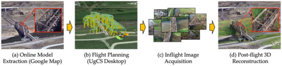
Figure 1.
Overview of truss bridge reconstruction based on the proposed method.
The obtained model is further processed to explore the camera/UAV search space around the bridge and the observable truss surface points for the subsequent view and path planning (Section 3). The proposed method first computes the optimal viewpoints that maximize the reconstruction quality at each observable surface point by selecting the best subset from an iteratively resampled candidate set (Section 4). The candidate is a set of densely sampled oblique viewpoints (i.e., multiple orientations at each position) initialized within the UAV free space while considering the camera/inspection parameters. After the optimization, the method converts the discrete viewpoints into single or multiple smooth flight trajectories subject to UAV constraints (i.e., aerodynamics, battery capacity, memory usage, and safety distance to the on-site objects) (Section 5). These trajectories are then transformed into the world coordinates (e.g., WGS84) and uploaded to the onboard autopilot system for the automated inflight image acquisition using single or multiple UAVs (Section 6.2). A photogrammetric reconstruction software will use the acquired high-quality images to generate a truss bridge’s geo-referenced, high-fidelity 3D model (Section 6.3).
3. Initialization
3.1. Input Parameters
Several important parameters must be defined as the inputs of the proposed method. In this study, we classify these parameters into four categories: (1) the UAV parameters, (2) the camera parameters, (3) the inspection requirements, and (4) the safety concerns. The UAV parameters include the physical properties of the selected UAV, such as the overall flight duration, the designed inflight speed, and the maximal number of executable waypoints in each flight. The camera parameters describe the properties of the onboard camera system, including the horizontal angle-of-view (AOV), the resolution of the onboard camera, and the gimbal pitch rotation limits. Because the in-plane rotations do not change the image contents, we locked the gimbal roll angle at and aligned the gimbal yaw with the UAV orientation. The inspection requirements are factors that control the quality of the collected images: they are the maximal/saturated GSD and the incidence angle. The safety concerns are parameters that define the UAV flyable space. They include the safe clearance to site objects, the minimum height above the ground level (AGL), and whether the UAV is enabled to fly through the truss. Fly-through-truss is a binary coefficient that defines whether the spaces within the truss structure are available for UAVs to pass through. These spaces enable the UAVs to inspect the truss bridge’s interior surfaces better. However, most consumer-grade UAVs cannot fly closely around metal structures (e.g., steel truss) because electromagnetic disturbances can affect the onboard sensing system (i.e., compass) and corrupt the GPS positioning capabilities. Therefore, for safety, we enable the fly-through-truss option only when the UAV onboard navigation system can handle the signal interference. The symbols, descriptions, and the default values of the parameters are listed in Table 2 below.
Table 2.
Summary of the input parameters, the symbols, the descriptions, and the default values.
3.2. Preprocessing
Based on the input parameters, the initial model extracted from Google Maps is pre-processed to define the UAV configuration space, the search space of the admissible viewpoints, and the truss surface points for visibility/quality evaluation.
3.2.1. UAV Configuration Space
The UAV configuration space is the free space accessible by a UAV. Due to the external noise (e.g., GPS errors, wind, signal interference, etc.), a safety tolerance (Table 2) between the model and the selected UAV must be maintained. Since the input model format is a triangular mesh, the space inaccessible by a UAV can be defined by extruding the safety tolerance along the normal at every surface of the mesh. New mesh surfaces (highlighted as orange in Figure 2a) that cover every side of the bridge with the defined tolerance are then constructed by connecting the adjacent extruded points. Positions located within this mesh or intersected with the mesh surfaces are considered collisions.
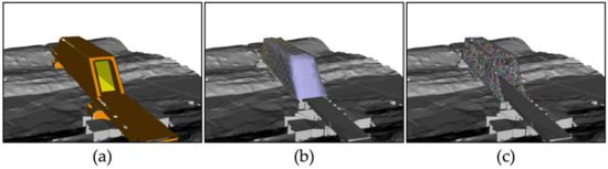
Figure 2.
Model preprocessing: (a) the surface meshes that define the UAV configuration space (colored in orange) and whether UAVs are allowed to fly within the truss (colored in yellow); (b) the resampled convex hull for candidate viewpoints sampling (only the exterior mesh is shown); (c) the truss surface points (randomly colored) that guides the subsequent viewpoints planning.
To define the free space within the truss, another surface mesh that covers the interiors of the truss structure (highlighted as yellow in Figure 2a) is developed. This mesh can be manually created or downscaled from the convex hull (detailed in Section 3.2.2). It is worth noting that this mesh is created only when the fly-through-truss option is disabled.
3.2.2. Viewpoints Search Space
The viewpoints search space is a subset of the UAV configuration space where the baseline observation quality of the collected images is guaranteed. Thus, only the free spaces surrounding the truss surfaces within certain distances should be considered. To achieve that, we performed the Quickhull algorithm [27] to generate a watertight convex hull that tightly covers the input truss. The convex hull was then resampled into a uniformly distributed triangular mesh using approximated centroidal voronoi diagram (ACVD) [28]. Figure 2b shows the triangle mesh for generating the candidate viewpoints set. For each triangular surface, a candidate viewpoint can be generated using the sampling-based coverage algorithm [15]. This strategy encourages the uniform sampling of the candidate set, which provides a good initialization for the subsequent optimization.
Please note that the candidate set only covers the exterior of the truss. To also sample the candidate viewpoints at the interior of the truss (when the fly-through-truss mode is activated), we reversed the normal of the convex hull and resampled the surface mesh. The result is a double-sided triangular mesh where viewpoints can be sampled within the free space at both sides of the truss. In this study, we set the interior/exterior convex hull to contain 100/500 triangle surfaces, respectively, for the candidate viewpoints sampling (Section 4.1).
3.2.3. Truss Surface Points
The surface points are visible points located at the surface of the bridge truss structure. These points are utilized to measure each viewpoint’s visibility and quality. Given the input model of the truss structure, Poisson disk sampling [29] was employed to sample the surface points at the model surfaces evenly. The normal of each point is computed as the average of the surface normal at each local Poisson disk. Figure 2c shows the sampled surface points at the truss surface.
4. View Planning
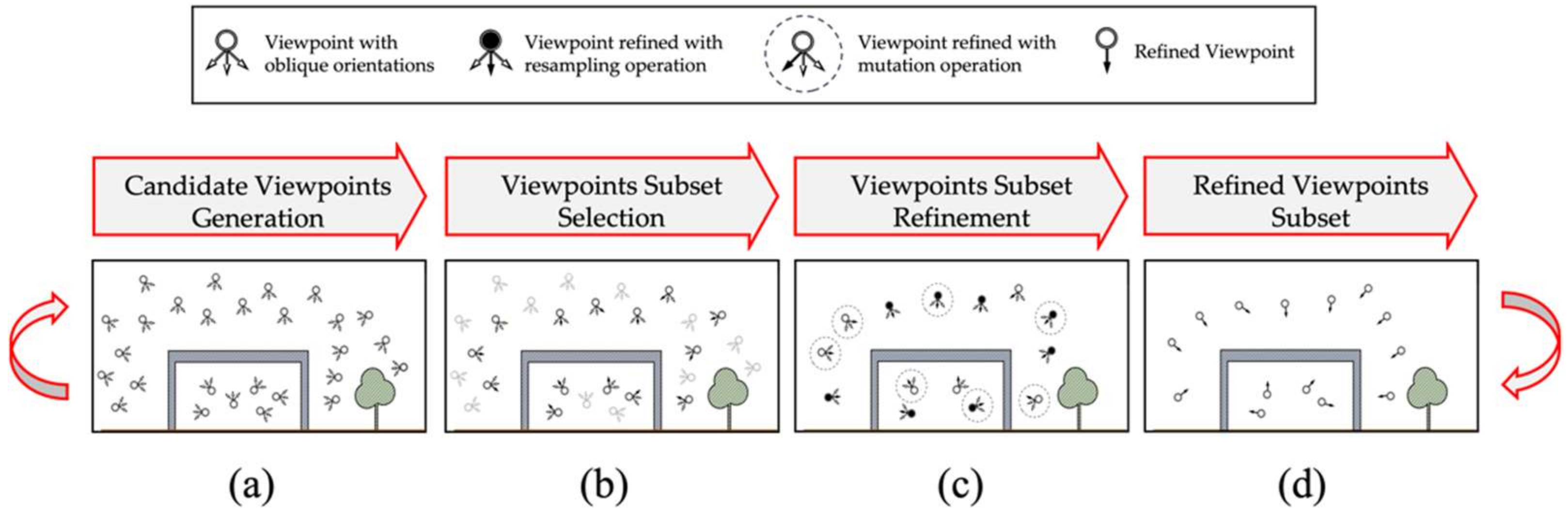
Figure 3 shows the workflow of the proposed view planning method. The method was developed in an iterative optimization schema: starting with a randomly initialized set of oblique viewpoints (i.e., multiple candidate view orientations at each sampled position) that covers the truss geometry (Section 4.1), the method selects (Section 4.2) a vantage viewpoint subset from the candidates based on the MVS geometric criterion. The selected subset is further refined to explore better solutions (Section 4.3) and then utilized to resample the candidate set for the subset viewpoints selection in the next iteration (Section 4.4). The above steps are wrapped into an adaptive particle swarm optimization (APSO) framework such that both the candidate and the refine subsets are iteratively optimized. The details of each step of the proposed method are discussed in the following paragraphs.
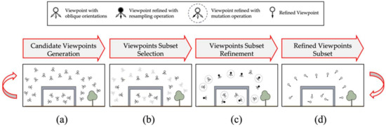
Figure 3.
Workflow of the view planning method: (a) Sampling a set of candidate viewpoints with added view orientations at each position; (b) Selecting the subset of the viewpoints from the candidate set (non-selected viewpoints are grayed out); (c) Refining the selected subset based on resampling (highlighted in black) and mutation (highlighted in dashed circles) operations; (d) The refined viewpoints are used to iteratively guide the resampling of the candidate viewpoints until the termination condition is met.
4.1. Candidate Viewpoints Generation
The candidate viewpoints are generated in two steps: (1) one admissible viewpoint is sampled within the search space of each triangle surface (i.e., convex hull); (2) multiple oblique orientations are added at each view position to enhance the searchability.
4.1.1. Admissible Viewpoints
Mathematically, let be a triangle surface of the convex mesh, we define a viewpoint is admissible if the following constraints are satisfied Equation (1):
where computes the GSD of a viewpoint to the surface given the camera FOV and image resolution, measures the incidence angle between the viewpoint and the normal of surface plane, and is the gimbal rotation angle. We set the initial orientation of each viewpoint as a ray casting from the viewpoint to the center of the triangle. is a binary function that measures if the designed viewpoint is located within the UAV configuration space (i.e., no collision). ensures the altitude of the viewpoint is AGL. These constraints formulate the viewpoint search space at each triangle surface.
4.1.2. Oblique View Orientations
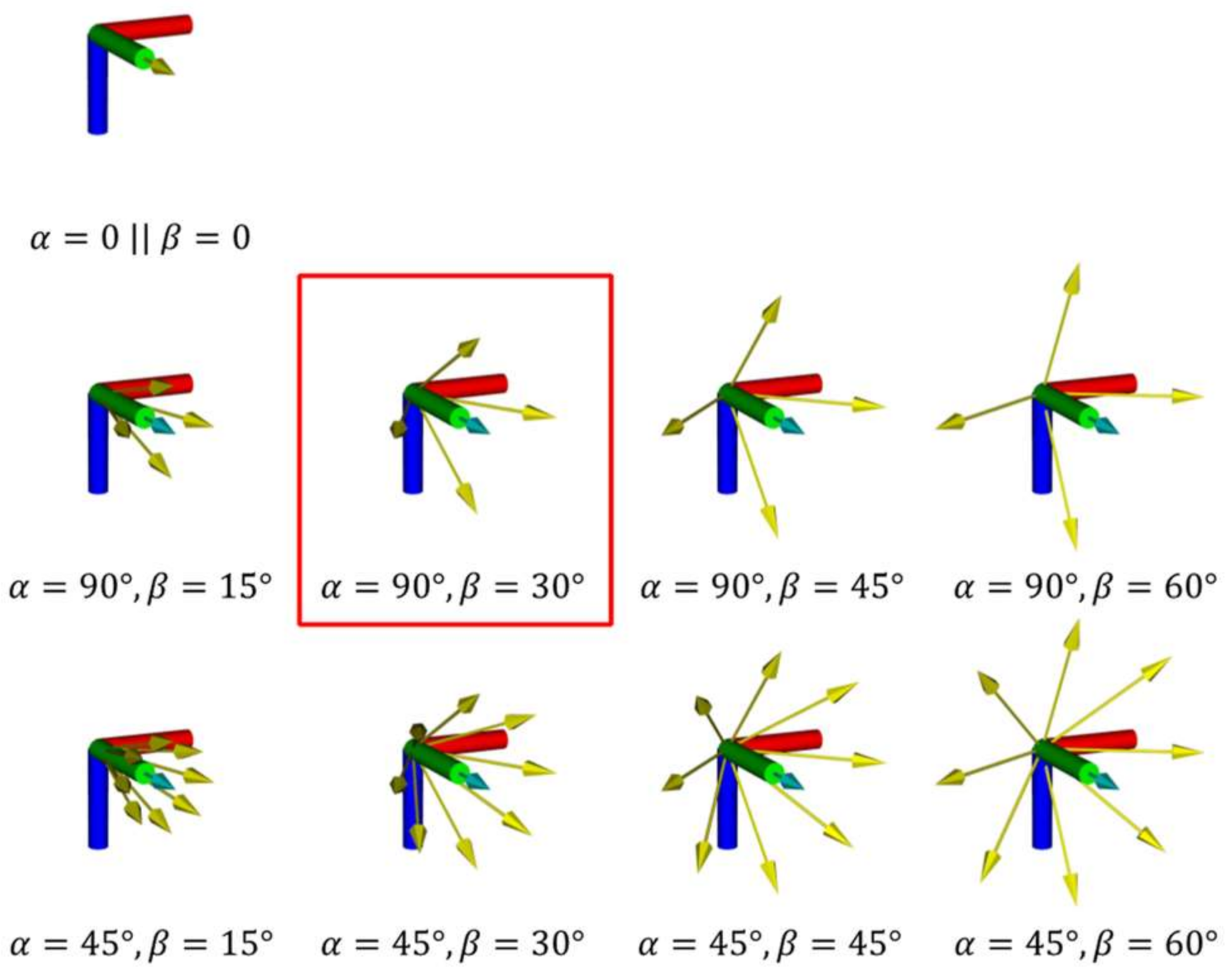
Due to the limited camera FOV and the complex truss geometry, a single view orientation might be insufficient to cover every truss surface. Thus, we add extra orientations at each sampled position to increase the searchability. Given the initial orientation of the admissible viewpoint, the oblique orientations are symmetrically generated based on two parameters: and . measures the adjacent angles between the extra orientations. The smaller of , the more oblique orientations are generated. denotes the angle between the original and the oblique orientation. The larger indicates the increased exploration ability of the oblique orientations. It is noted that the oblique orientations must also follow the gimbal constraints, and the orientations with the pitch angle located outside the gimbal limits must be rejected. Figure 4 illustrates the oblique orientations (arrows in yellow) generated under the selection of different and . In this study, we set and based on the experiments (detailed in Section 7.4.3).

Figure 4.
The collection of oblique orientations (arrows in yellow) from the initial one (arrow in cyan) based on the combination of different and . Highlighted is the selected combination based on the experiments.
4.2. Viewpoints Subset Selection
The initially sampled candidate set contains a redundant number of viewpoints. In this section, we describe how to select the best subset from the candidate viewpoints. The method is developed based on the multi-view stereo quality insurance principle that only the geometric consistent images contribute to the final reconstruction [30]. In the following paragraphs, we first present the quality-efficiency metric that measures the reconstruction quality given a set of ordinary viewpoints (i.e., one view orientation at each position). The metric also identifies/ranks the contribution of each viewpoint. Next, we propose a greedy view selection algorithm to efficiently select the best subset from the candidate oblique viewpoints based on the metric.
4.2.1. Quality-Efficiency Metric
The quality-efficiency () metric is formulated as the weighted sum of the reconstruction quality () and the reconstruction efficiency () as Equation (2) below:
where is a constant coefficient that balances these two terms. In this study, we set based on a thorough experiment (detailed in Section 7.4.3). The presented metric encourages high-quality reconstruction from a small set of viewpoints to be obtained. In the following, we discuss the computation of each term in detail.
Reconstruction quality predicts the MVS quality at each surface point given a set of viewpoints. Due to the absence of the pixel-level contents at the planning phase, the metric is computed based on the geometric priors at the image level [30,31] where the following principles are considered:
- Principle 1.
- Each surface point must be covered by at least two high-quality images in terms of sufficient GSD and the incidence angles for feature extraction and matching.
- Principle 2.
- Small baselines between the matched images can cause large triangulation errors for depth interpretation.
- Principle 3.
- Redundant images are uninformative views that do not reduce the depth uncertainty while can increase the computation workload.
Based on the above-mentioned principles, we formulate the quality metric as Equation (3) below:
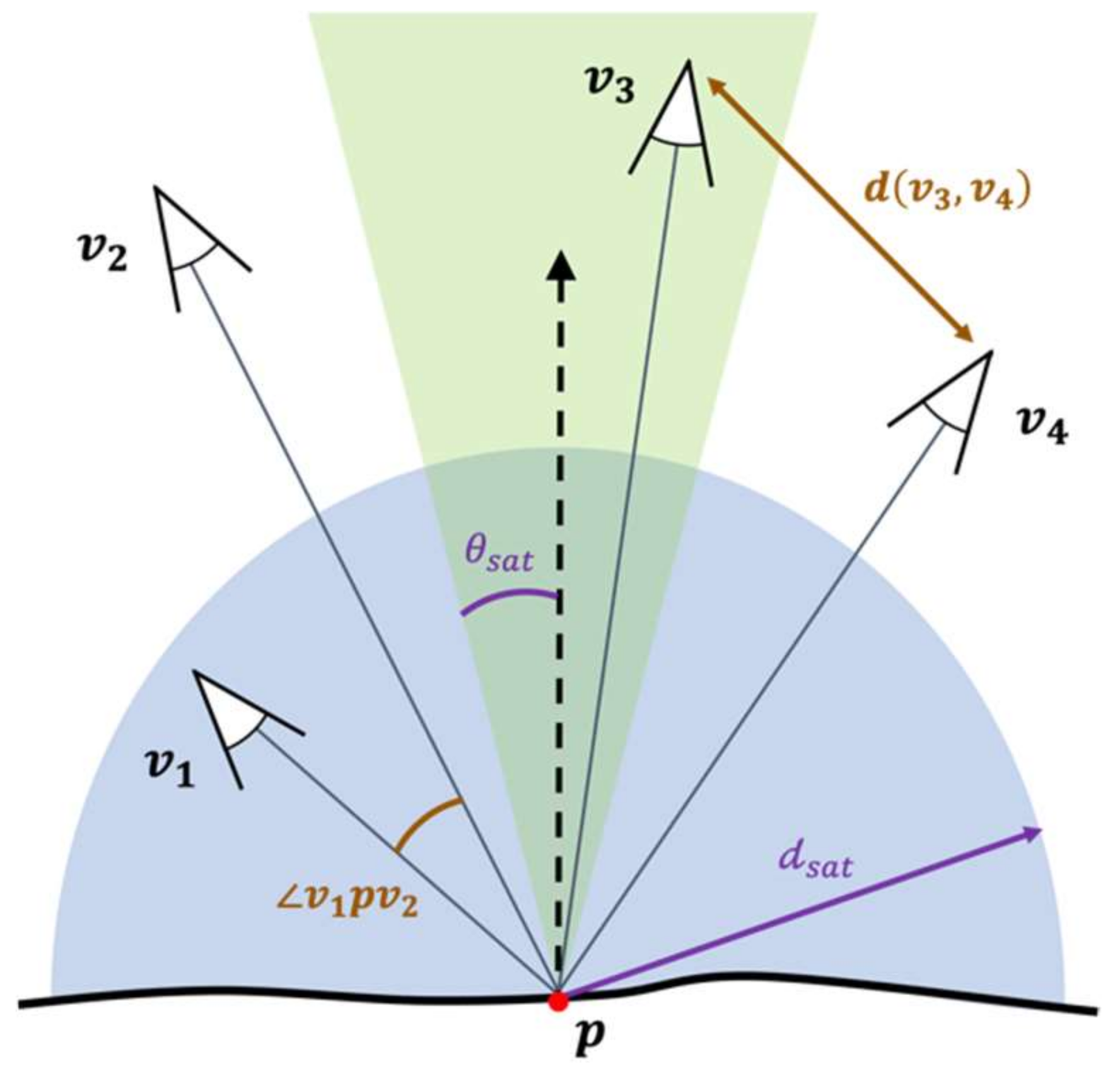
where measures the quality of a truss surface point as the sum of the k best observations (Principle 3). We set k equal to 3 due to the increased robustness of the three-view reconstructions at texture-less surfaces [32]. is a binary function that detects if the point is visible from . measures the observation quality of each viewpoint, which is computed as the average () of two factors: (1) the view-to-point distance; and (2) the view-to-point incidence angle (Principle 1). These two factors are normalized and saturated based on the input parameters. denotes the subset of viewpoints where the baselines at follow the stereo-matching constraints (Principle 2). Based on [33], we empirically set in this study. Figure 5 illustrates the geometries of the viewpoints to a surface point.
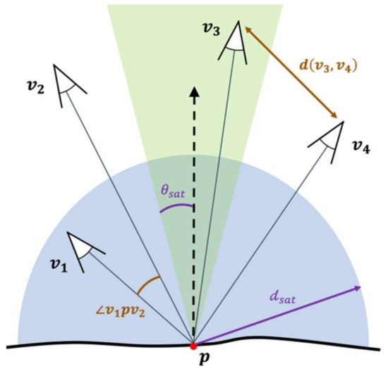
Figure 5.
The geometry between a set of viewpoints and a surface point where , . (The shaded regions respectively denote the spaces formed by the saturated angles (in green) and the saturated distances (in blue).)
Reconstruction Efficiency measures the ratio of the non-selected viewpoints over the complete viewpoints set (as in Equation (4)). This metric encourages reducing the redundant images for efficient aerial reconstruction.
where is the quality of the viewpoint to every surface point . is the subset of that contributes to the reconstruction quality (with ).
4.2.2. Greedy Views Selection
Selecting the viewpoints subset from an oblique set involves the selection of the viewpoint positions as well as the best orientation at each position. Clearly, enumerating every possible combination is expensive. To make the problem tractable, we propose a greedy algorithm that includes three steps as follows:
- Step 1.
- Measuring of the oblique viewpoints with the initial orientation at each view position (Section 4.2.1). The output subset is considered as the baseline for the view selection in the next step.
- Step 2.
- Selecting one viewpoint in the baseline and substituting the current orientation with one oblique orientation. The current orientation of the viewpoint is updated if is increased. Iterative this process to all oblique orientations at the position.
- Step 3.
- Repeating Step 2 at every viewpoint in . Stop the operation until every viewpoint has been visited or the overall quality does not increase a certain number of times (i.e., 5).
Clearly, the sequence of the viewpoints being selected (as in Step 2) significantly affects the outcome. To avoid the results being biased to a bad sequence, we perform multiple runs of Step 2 in parallel with the viewpoints selected in random order at each run. Among the different runs, the viewpoints subset with the maximal is chosen as the output of the algorithm.
4.3. Viewpoints Subset Refinement
The viewpoints subset refinement is to perform the local search to better exploit the problem space. The main idea is to adjust the viewpoint in where is low. The proposed refinement method is performed based on two operations (as in Figure 3 (c)): In the first operation, we resample the viewpoints with quality less than a pre-defined threshold (i.e., 0.2). The viewpoints are updated if is increased. In the second operation, a ratio (i.e., ) of the viewpoints with the lowest quality in are selected and incrementally mutated at positions within a defined radius (i.e., 5m). We update the mutated viewpoint if the is increased. Preliminary results showed that this refinement step can improve the at an average of 6–8% in each iteration without increasing the size of .
4.4. Candidate Viewpoints Resampling
The refined subset is near-optimal only if the candidate set covers or partially covers the true optimal viewpoints. However, enumerating every possible candidate in the 3D continuous space is impractical due to the scale and the geometric complexity of the truss structures. Thus, we iteratively resample the candidate viewpoints such that the randomly initialized candidate set eventually converges to the optimal or near-optimal solutions (i.e., cover the optimal viewpoints). In this study, we wrap the resampling procedure into the APSO framework [34]. Compared to the conventional PSO, APSO is selected due to the increased convergence speed and exploitability in solving multimodal optimization problems. Specifically, we define each candidate set (Section 4.1) as a particle and the quality-efficiency metric of the refined subset (Section 4.2) as the fitness. Equation (5) shows the resampling mechanism based on APSO.
where is the position of a viewpoint, is the particle velocity at . denotes the number of iterations, and is the global best particle (i.e., viewpoint subset with maximal ). and are coefficients that control the update behavior at each viewpoint. is a standard normal distribution along each axis of the Euclidean space. is the function that measures the difference between the position of a viewpoint in a particle and the correspondent position in the global best (i.e., viewpoints at the same triangle surface). We set the function to return 0 if the viewpoint does not belong to . Notably, the presented Equation (5) only updates/resamples the positions of the viewpoints. The initial and oblique orientations at each updated position need to be recomputed afterward using the same strategy as in Section 4.1.
5. Trajectory Planning
This section converts the optimized viewpoints into the UAV executable trajectories (as shown in Figure 6a). The method starts with constructing a complete, undirect graph, with each node indicating the position of a viewpoint and each edge as the distance of the collision-free path between every pair of the view positions. As shown in Figure 6b–d, the edge distance between each pair of the viewpoints is computed in three steps: (1) Connect the viewpoints with a straight line and check if this line collides with the on-site obstacles; (2) If a collision is found, the informed rapidly exploring random tree star (RRT*) [35] is employed to efficiently reroute the path. If the path does not converge a given number of iterations, we recognize the path segment as not accessible, and a significant penalty is assigned to the edge. (3) For each rerouted path, B-spline curve interpolation [36] is applied to smooth the path segment for the UAV path following at the desired speed. The distance of the smoothed path is then measured as the cost of the edge between the viewpoints.
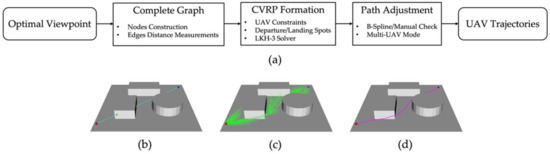
Figure 6.
The flowchart of UAV trajectory planning (a) and the detailed steps of the edge distance measurements procedure (b–d): (b) connect start (dot in red) and end (dot in blue) waypoints with straight line, check if collisions exist (dot in green); (c) perform informed RRT* (in green) to reroute the path (in purple); (d) smooth the collision-free path using B-spline curve interpolation.
Based on the constructed graph, the trajectory planning problem is then formulated as a capacitated vehicle routing problem (CVRP) [37]. To simplify the problem, we set the vehicle type and capacity as homogeneous, and let the routes start and end at the same spot (i.e., drone departure/landing). Two factors are considered the major capacity constraints of the problem. The first is the UAV battery capacity, which is a determinant of how long can the UAV stay in the air. The second is the autopilot limitation, which restricts the maximal number of waypoints to be uploaded per flight. Many autopilot systems (e.g., DJI) have such constraints for safety concerns. Unlike the battery constraint, the waypoint limit does not require the UAV to land, but needs the drone to be located in proximity to receive the users’ input signal for continuing the mission.
In this study, we employ the Lin–Kernighan–Helsgaun (LKH-3) [38] as the problem solver. The solver utilizes the improved symmetric transformation and five-opt move generator to efficiently compute the paths while handling the battery/memory constraints. The output is single or multiple routes, each route starts/ends at the same spot and travels through a subset of viewpoints under the imposed constraints. It is possible that the outputted paths still contain sharp corners that may not be tightly followed by the UAV at the desired speed. Under such conditions, the path can be either re-smoothed using the B-spline algorithm or manually checked/adjusted by the operator at the pre-flight stage. While the presented method is initially developed for a single UAV to sequentially fly the paths (with battery replacement). The method can be easily extended for multiple UAVs to fly in parallel by adjusting the flight speed of the UAVs at regions where the paths are intersected [39].
6. Implementation Details
In this section, we discuss the implementation details of the proposed method, including the visibility detection for quality evaluation, the procedures of automated flight execution, and the 3D reconstruction pipeline.
6.1. Visibility Detection
For each viewpoint, we compute the visible surface points to evaluate the correspondent contribution to the quality metric. The presented visibility detection method considers not only the occlusions as is mostly done, but also the inherent image triangulation properties. This strategy reduces the computation load and avoids considering the poorly matched camera views. Given the camera parameters (as in Table 2), we construct a viewing frustum to simulate the camera FOV at each viewpoint. The visibility detection is performed in three steps:
- Step 1.
- We examine every surface point by checking whether the point is located within the frustum.
- Step 2.
- We cast a ray from the viewpoint to each surface point within the frustum and check whether the ray is intersected with any truss components. The surface points without intersections are visible from the viewpoint.
- Step 3.
- For each visible point, we measure the incidence angle between the point normal and the camera ray. Only the points with incidence angles smaller than a predefined angular threshold ( ) are triangulable by the viewpoint.
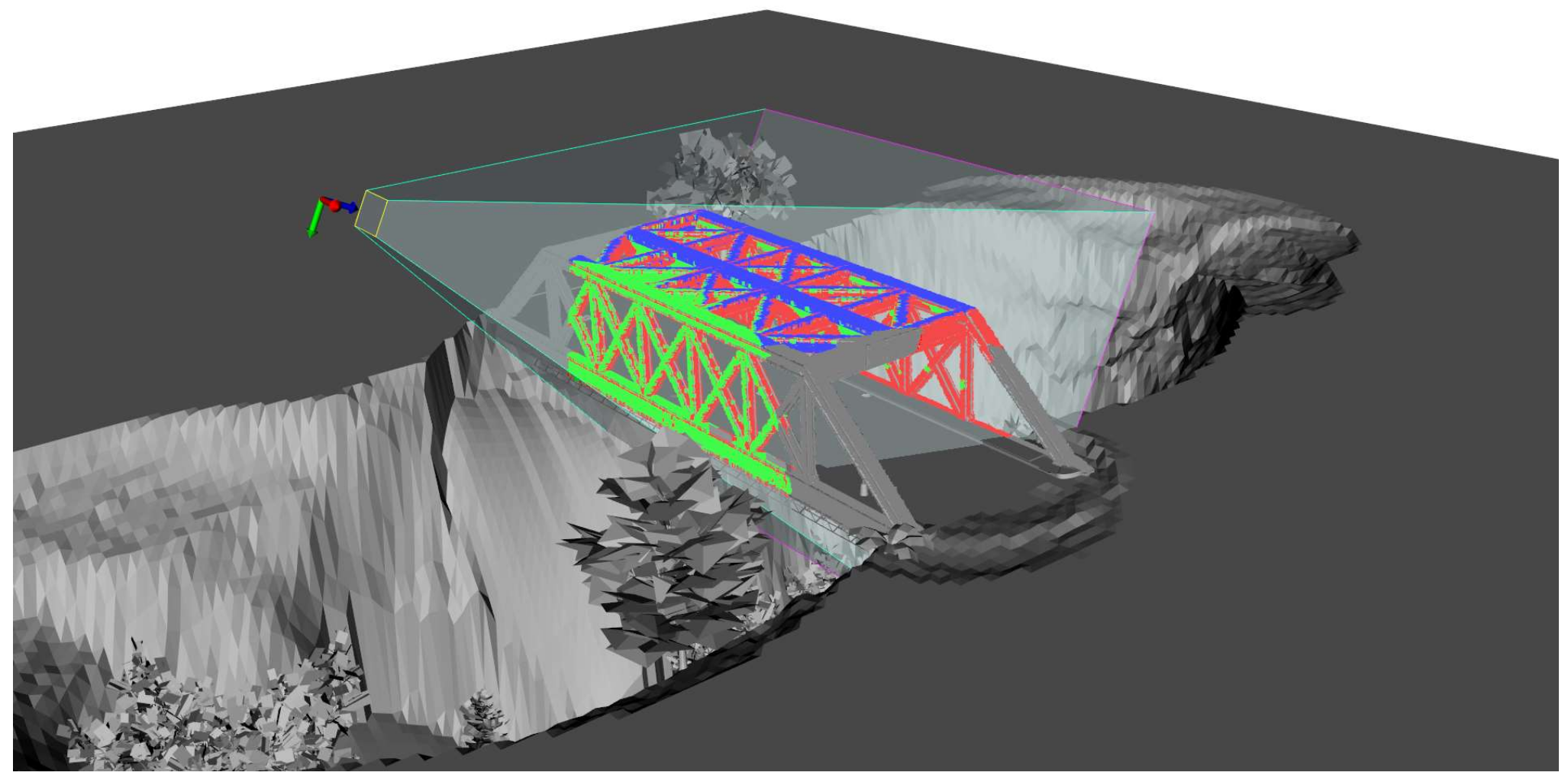
Figure 7 illustrates the proposed visibility detection using a single viewpoint and a synthetic truss bridge. In this study, the visibility detection is implemented based on Octree-based collision detection [40] using VTK [41].

Figure 7.
Visibility detection method: The surface points in red are covered by the camera FOV (i.e., viewing frustum) but not visible (i.e., occluded by other structures); The surface points in blue are visible by the camera view, but the incidence angles are too large, which might result in poor image matching results; The points in green are visible and triangulable that passes the visibility detection.
6.2. Flight Execution
Because the flight trajectories were originally computed in the local coordinates, they need to be transformed to the World Geodetic System (WGS84) to be executable by a UAV. To achieve this, several ground control points close to the truss bridge to be inspected are manually surveyed using a GPS receiver. The transformation can then be found by correlating these GPS positions to the correspondent points in the local coordinates. Due to the relatively small scale of most bridges, rigid body transformation (i.e., assume the surface is flat) is used to map the transformations from the local coordinates to WGS84.
After the transformation, the viewpoints are uploaded into UgCS [42], a ground station software, for the automated inflight waypoints following and image acquisition. The software contains a hardware-in-the-loop simulator that can perform the pre-flight check before the field deployment. In this study, we use the DJI Inspire 1 as the flight platform to execute the missions, and the DJI Zenmuse X3 for the aerial image collection. Inspire 1 can fly for around 15 min when the wind speed is moderate. We restrict each flight to only use at most 80% of the battery capacity (i.e., 12 min) for safety concerns. It is noted that DJI drones have the limit of at most 99 waypoints to be uploaded per flight, which is another capacity constraint to be considered in the trajectory planning (Section 5).
6.3. 3D Reconstruction
After the flight executions, the collected aerial images are imported into 3D reconstruction software. In this study, Agisoft Metashape [43] is selected since it has been previously used for the 3D reconstruction of bridge structures with fewer artifacts [1]. When the GPS of each image is available, reference matching is enabled to accelerate the image alignment process. To obtain the detailed reconstruction, we set the quality of both the image alignment and dense point cloud as high with the depth map as aggressive to actively filter out the noises in the final reconstruction.
7. Evaluation
7.1. Experimental Setup
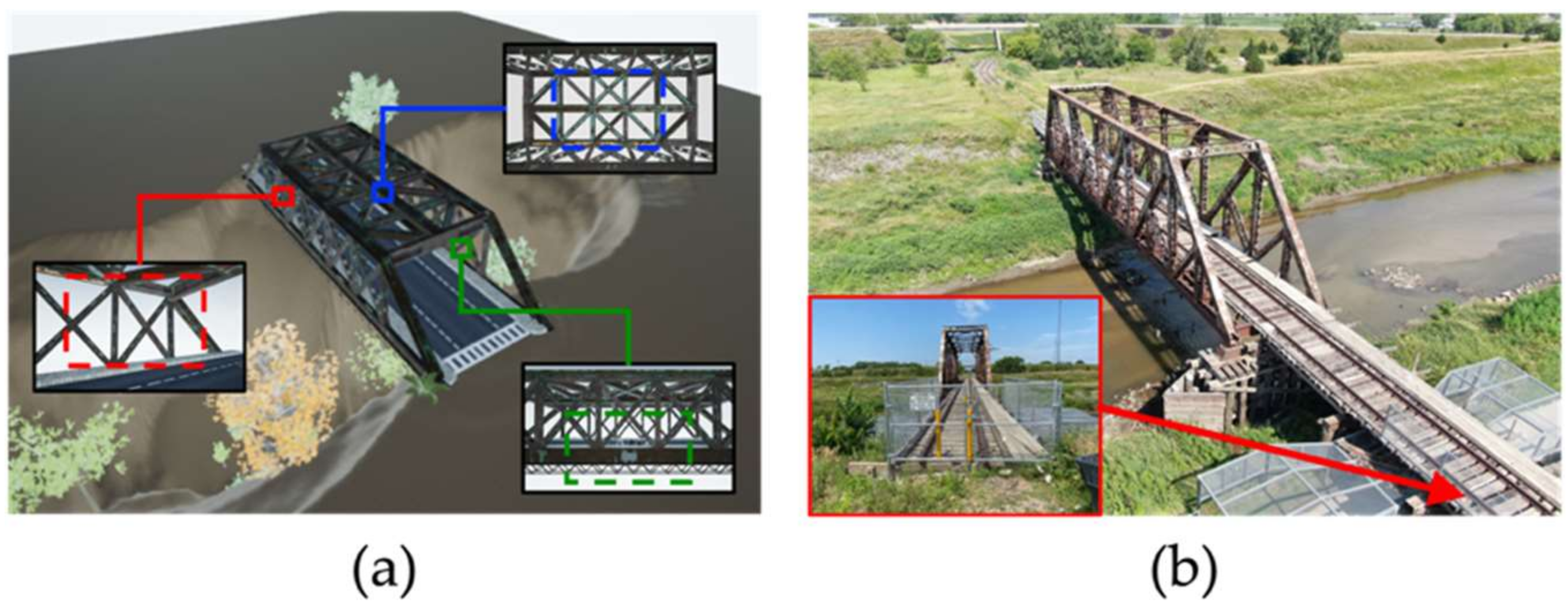
The performance of the proposed method is evaluated based on both a synthetic and a real-world truss bridge. Evaluation using the synthetic bridge has the advantage of controlling the environmental factors (e.g., reflection, illumination change, shadows, moving objects, etc.), which are often considered as noises in image-based reconstruction. In this study, Unreal Engine 4 (UE4) is selected to render the synthetic environment due to its ability to provide photo-realistic scenes at high levels of details (LoDs). UnrealCV [44], an open-source computer vision SDK, is employed to render the image at each camera footprint. The selected synthetic truss bridge (as shown in Figure 8a) is a highway bridge across a valley. The bridge truss structure, which was downloaded from the Unreal Marketplace [45], has a dimension of . It is noted that the original package only contains the bridge superstructures; we import the deck surface and the surrounding environment to simulate the real-world condition. Because the synthetic environment is noise-free, the fly-through-truss option is enabled () in the evaluation.

Figure 8.
(a) Synthetic truss bridge and the detailed views of the selected regions; (b) the abandoned truss bridge to be surveyed, which is restricted to human access due to safety concerns (the detailed view).
The selected truss bridge for the real-world experiment is an abandoned railway bridge (as shown in Figure 8b). The bridge has a dimension of which is not accessible by the human at the time of the inspection due to safety concerns. It is noted that the inner space of the bridge is insufficient for the UAV to pass through (i.e., safety tolerance), even without considering the magnetic interference. Thus, the fly-through-truss () is disabled in the real-world environment.
7.2. Comparison
Based on the authors’ knowledge, there is no reported flight planning method specifically designed for the 3D reconstruction of truss bridges. Thus, a baseline and a state-of-the-art method for building reconstruction are selected to evaluate the performance of the proposed method in the simulated environment. In this study, the Overhead flight, composed of an orbit path with the camera surrounding the center of the scene followed by a lawnmower path providing the bird views, was selected as the baseline approach. This path can be easily reproduced using commercial flight planning software [42,46,47]. The overlap between the adjacent viewpoints is 80% to ensure dense image registration. The NBV method presented in [17] is employed for the state-of-the-art approach. The method incrementally adds the viewpoints with the largest marginal reward from a graph of the candidate cameras. The orbit path obtained from the Overhead flight is used to initialize the optimization. Compared to our method, the original implementation of [17] used different strategies and implementation libraries for the space representation (i.e., occupancy map), the collision detection/avoidance, and the visibility detection that might affect the result. To avoid confusion, we implement the NBV using the exact implementation strategies as our work such that the final results are only affected by the optimization algorithms. The method [17] limits the viewpoints planning in a single flight (i.e., battery constraints) that might result in incomplete reconstruction. Thus, in the simulation, we set UAV flight time as unlimited and leave the evaluation of the trajectory planning to the field experiment.
For the field experiment, both the reconstruction quality as well as the efficiency of the inflight image acquisition and the post-flight image processing are discussed. Thus, we select a sweep-based, multi-UAV-supported route planning method [23] as the previous state-of-the-art. The method designed three routes to tightly cover the structure from different perspectives while considering the photogrammetric constraints (i.e., GSD, camera angles, overlapping, etc.). Due to only one UAV being available (i.e., DJI Inspire 1) in the field experiment, the planning adjustment step (for multi-UAV cooperation) was skipped. Since the method does not include the collision avoidance algorithm, a manual check is needed to guarantee the safety of the mission. All the experiments were executed on a PC desktop with Intel CPU E5-2630, 64G memory running on Ubuntu 18.04.
7.3. Quality Evaluation
Evaluation of the reconstruction quality includes a visual and quantitative comparison. The visual comparison focuses on the observations of the texture smoothness and the artifacts in each reconstruction, especially in the complex geometric regions (e.g., truss interiors, connections, and slim beams). The quantitative evaluation measures the geometric fidelity between the reconstruction and the ground truth. The evaluation includes three major steps: First, the reconstruction model is cropped and filtered only to contain the regions covered in the ground truth (i.e., truss bridge). Second, a coarse-to-fine alignment is used to transform the coordinates of the reconstruction into the ground truth. The coarse alignment is performed by the rigid transformation from a set of correspondence points. Based on the coarse alignment, the fine transformation is computed using iterative closest point (ICP) registration [48]. It is noted that the reconstructed models might contain outliers. Thus random sample consensus (RANSAC) [49] is employed such that the refined transformations are robust to such outliers. Third, the F-Score, as presented in [50], is used to measure the fidelity of the finely aligned model. F-Score is composed of the harmonic mean of two indicators: Precision, and Recall, given a distance threshold. Precision measures the accuracy of the reconstruction by averaging the errors of each reconstructed point to the ground truth. In contrast, Recall evaluates the reconstruction completeness by measuring whether each point in the ground truth is covered by the reconstruction. A high F-Score indicates a reconstruction that has both high model accuracy and completeness. The formula of F-Score , Precision , and Recall are presented in Equation (6) below. We refer the readers to [50] for the details of the indicators. Due to each F-score being computed with a distance threshold, thus we report the quantitative evaluation based on the F-scores across a range of distance thresholds .
where and respectively, denote the points set of the source and the target models. is the error metric that measures the distance of a point in the source model to its closest point (represented as *) in the target model.
For the synthetic bridge, the ground truth model is known. Thus, the F-score can be directly computed by comparing the reconstruction to the ground truth. For the field experiment, terrestrial laser scanning (TLS) is used to obtain the ground truth model of the bridge. In this study, the Leica BLK360 laser scanner is selected. The scanner can obtain millimeter accuracy at a distance of fewer than 10 m, which is sufficient to obtain a high-fidelity 3D model of the truss bridge. Figure 9 shows the 2D view of the TLS scanned truss bridge and the on-site scanning spots. The 3D model is registered from 27 scans, with most of the scans conducted on the bridge. The entire survey took around four hours for on-site data collection and another five hours for the offsite data transmission and point cloud registration.
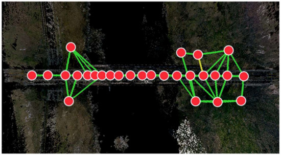
Figure 9.
A 2D view of the terrestrial laser scanned truss bridge. The 27 red dots denote the positions at each scan, and the links indicate the registration between the scans. The colors of the links denote the overlapping quality between the scans (Green: at least 75% overlapping; Yellow: at least 50% overlapping).
7.4. Results
7.4.1. Synthetic Bridge
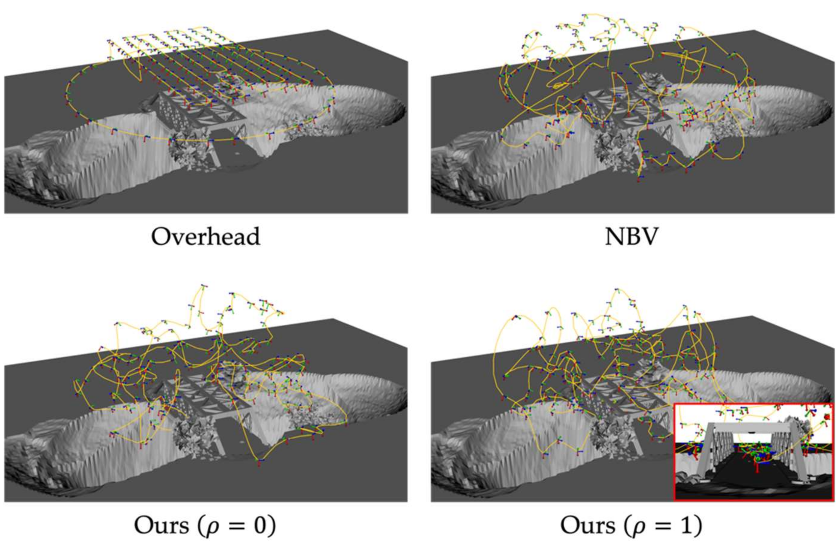
Figure 10 shows the trajectories computed using the Overhead, NBV, and our method () on the synthetic bridge. To make a fair comparison, we restrict the upper bound of NBV as the number of images generated with our method, such that the methods generate the same number of images. It observed that Overhead and NBV only compute the viewpoints surrounding the truss geometry. Instead, our method () enables the trajectories to pass through the truss (detailed view in Figure 10), and provides better observations of truss interiors. Table 3 summarizes the statistic of the runtime of flight planning, number of images, and the flight distance computed with each method. Clearly, Overhead requires significantly less running time with a fewer number of images and the flight distance needed when compared to other methods. Compared to the NBV where the candidate viewpoints are fixed, our method iteratively optimizes the viewpoints in the continuous space at the cost of the longer runtime. In addition, setting equal to one increases both the runtime and the number of images. However, because the proposed method can be computed offsite at the pre-flight stage, the increased runtime might cause minimal effects on the field deployment.

Figure 10.
The viewpoints and the trajectories generated using different methods.
Table 3.
The comparison of the runtime, number of images, and the flight distance on the synthetic bridge.
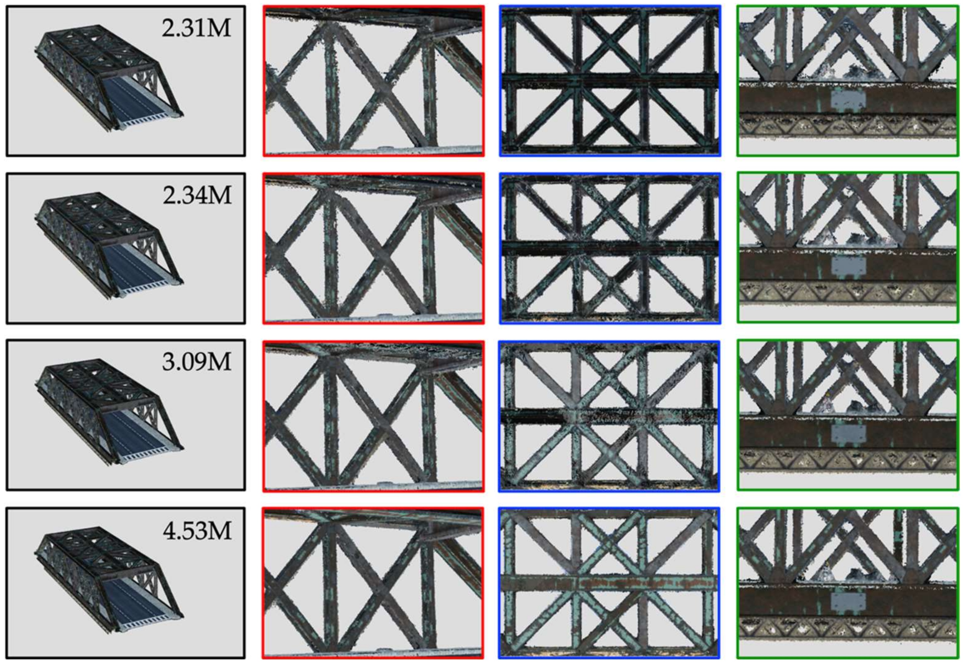
Figure 11 shows the visual comparison of the reconstructions using different methods, including the detailed views of three challenge areas as highlighted in Figure 8a. The results showed that our method () generates more visually appealing results at vertical/diagonal web members and the surface connections (second and fourth columns in Figure 11) when compared to both the Overhead and the NBV. In addition, the textures at the interiors of the top chords/struts (as third column in Figure 11) are only recovered by our method, especially when equals one. Table 4 presents the measured F-Score at varied distance thresholds (). The results validate the observations that our method outperforms the other two at every distance threshold. Enabling the fly-through-truss option shows the best result, which indicates that collecting the images from the inside of the truss can indeed improve the overall reconstruction quality.
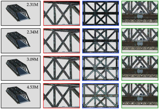
Figure 11.
The full-bridge view (first column) with the number of points (M: Million) and the detailed views (second, third, and fourth columns) of the 3D reconstruction of the synthetic bridge using different methods. First row: Overhead; second row: NBV; third row: Ours (ρ = 0); and fourth row: Ours (ρ = 1).
Table 4.
Quantitative comparison of the synthetic truss reconstruction between different methods.
7.4.2. Real-World Bridge
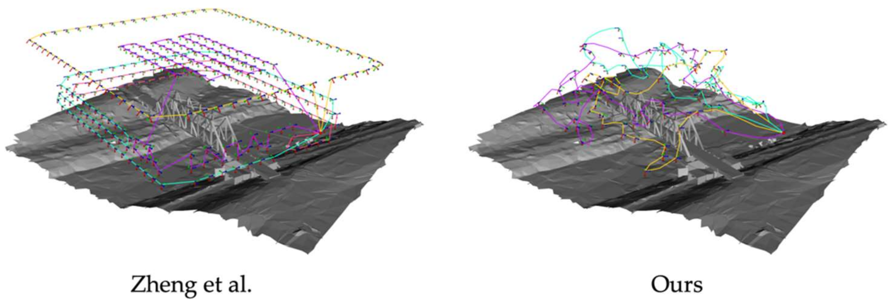
Figure 12 compares the flight trajectories computed with Zheng et al. [23] and our method. Because Zheng et al. [23]’s method was originally developed for the 3D reconstruction of building structures; the method takes more images. Table 5 shows the statistics of both the inflight inspection and the post-flight reconstruction. Clearly, our method takes shorter time both on-site and offsite.

Figure 12.
The flight trajectories using Zheng et al. [23] and our method. The colors denote the trajectories of different UAVs/flights for the mission execution.
Table 5.
Comparison of the statistics on flight execution and 3D reconstruction.
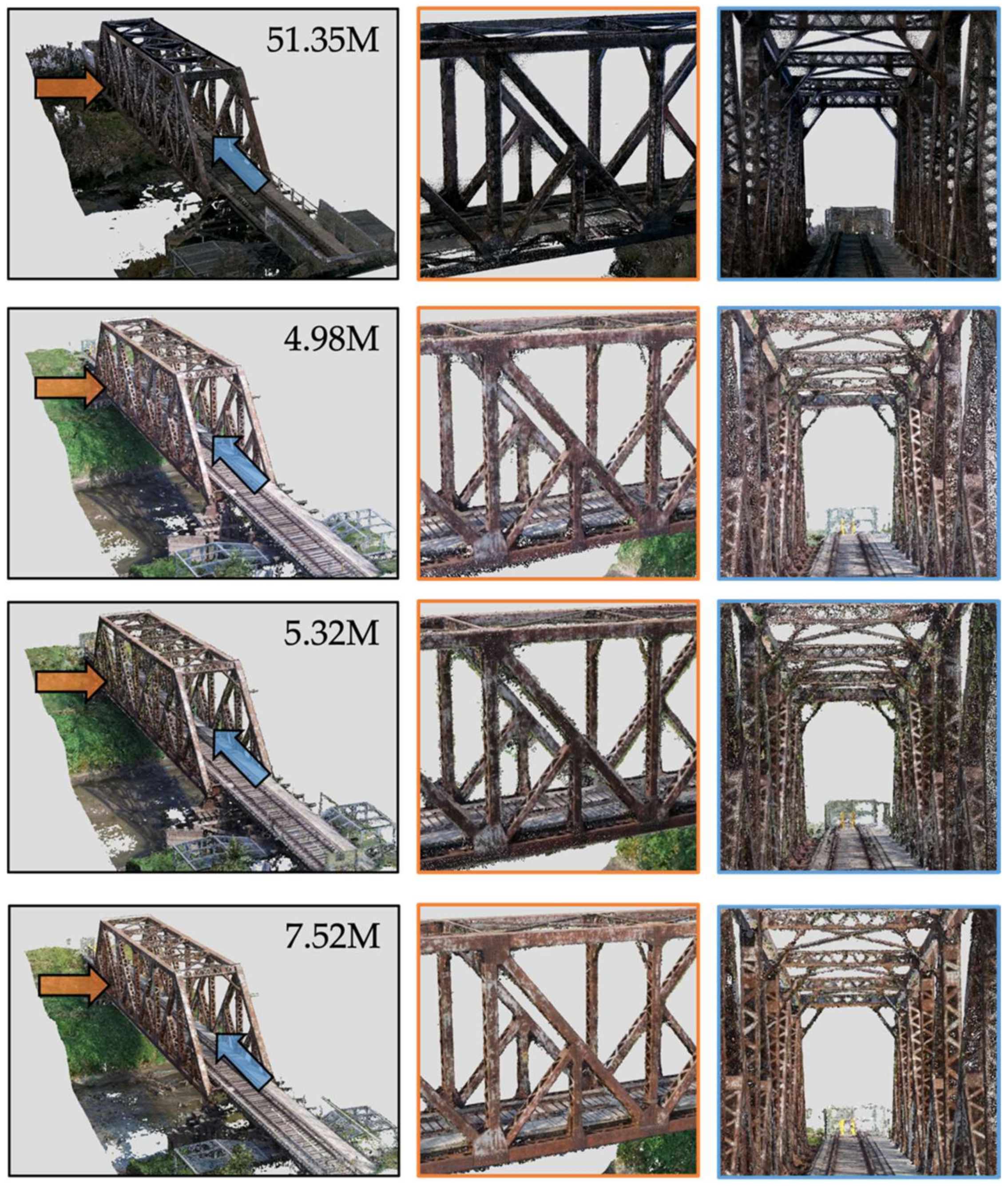
In Figure 13, a detailed comparison between the reconstructed models and the laser-scanned model is presented. Since the TLS model is obtained by scanning the bridge interiors, it shows the different color intensities when compared to the photogrammetry, where the images are taken from the external side. To make a fair comparison, the models need to be reconstructed from a similar number of images. Thus, we generate the reconstruction model with images taken only at routes 1 and 3 in Zheng et al.’s method [23]. The selected routes form similar flight patterns as the Overhead that can be utilized to represent the typical flight in the real-world experiment. The routes generate a total of 133 images, which is close to ours. It is evident that although both methods recover the major truss structures. The model obtained from routes 1 and 3 presents the worst result in terms of the point cloud density and recovering the model details (e.g., slim beams, joints, and truss interiors.). The low density of the point cloud shows the insufficient coverage at the truss surface. Compared to Zheng et al. [23], our reconstruction has higher density and preserves more structural details with much fewer artifacts. For example, the holes in the top chord and the boundaries of the diagonal beams are much better recovered by our method (detailed views in the third column in Figure 13). Table 6 presents the F-Score of the truss reconstructions as opposed to the TLS. The results demonstrate that our method slightly outperformed Zheng et al. [23] in terms of both the Precision and Recall, with less than half of the images being used, which validates both the efficiency and effectiveness of the proposed method.
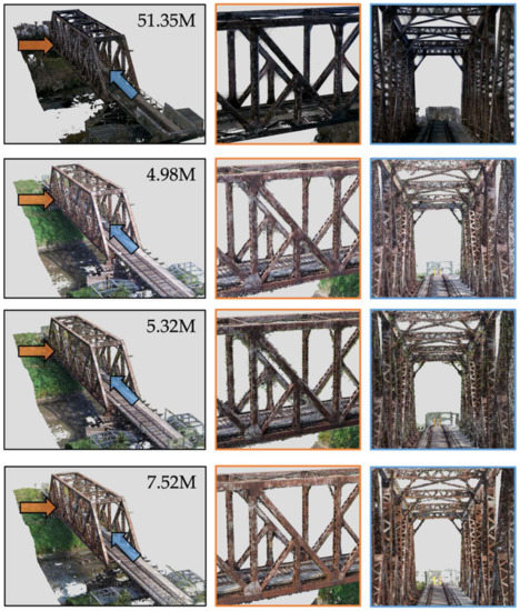
Figure 13.
The full-bridge view (first column) with the number of points (M: Million) and the detailed views (second, third columns) of the final reconstruction of the real-world truss bridge. First row: TLS; second row: Zheng et al. [23] (Routes 1 and 3 only); third row: Zheng et al. [23]; and fourth row: Ours.
Table 6.
Quantitative comparison of the real-world truss reconstruction.
7.4.3. Further Results
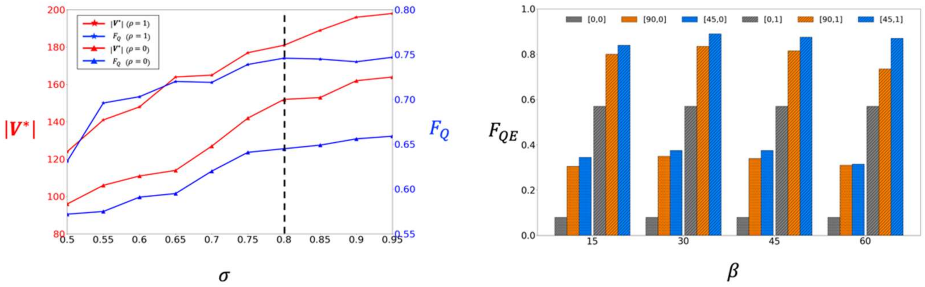
In this subsection, we evaluate the performance of several parameters based on the results from both the synthetic and the real-world bridges. First, the effects of the weight coefficients on the optimization performance is evaluated. Figure 14 (Left) shows the quality metric and the number of collected images under different . The figure showed that in contrast to which increases monotonically as , gradually decreases when close to one. Such results might be affected by the fact that the over-redundant images can cause diminished return. Because a smaller number of images is preferred for efficient reconstruction, we set the weight coefficient at 0.8 as a good trade-off between the reconstruction quality and the efficiency. Next, we evaluated the selection of the oblique orientations to the quality-efficiency metric . As shown in Figure 14 (Right), compared to the conventional viewpoints , using oblique viewpoints significantly improves for all test cases (for both or ). The result indicates that the oblique orientations indeed increase the reconstruction quality. Among the different combinations of and , we found the combination of and shows the best result. Thus, we select it as the default in the experiments.
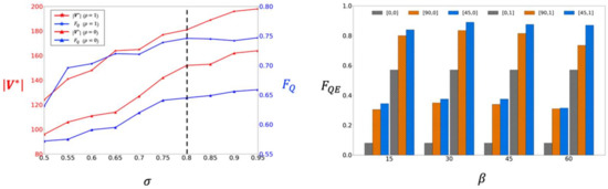
Figure 14.
Left: The values of and when different are selected; Right: The values of under different combinations of . The legend denotes .
8. Conclusions
This paper presents a new flight planning method for autonomous, efficient, and high-quality 3D reconstructions of truss bridges. The synthetic experiment showed that the proposed method outperforms the state-of-the-art NBV method with increased reconstruction accuracy and completeness. Enabling the fly-through-truss option significantly improves the coverage and model quality at the truss interiors, such as the top chord and other web members. The real-world experiment demonstrated that the presented method computed the image capture views can achieve a higher reconstruction quality with less than half of the images being used when compared to the existing sweep-based method. The planned trajectories ensure the safety of the flights while considering the UAV constraints, enabling the automated and efficient bridge inspection practice.
In this study, the authors extracted the input model from Google Maps to guide the viewpoints and trajectories planning. This strategy enables the flight plans to be designed offsite, reducing the survey time when compared to the existing literature. The presented method also accepts other types of 3D models, such as aerial photogrammetry, with minimal adjustment. This flexibility potentially enables the method to be performed as an incremental procedure by sending the outputted reconstruction as the input model for flight planning in the next iteration until the users satisfy the results.
Future works include evaluating the proposed method with the fly-through-truss option enabled in real-world experiments, which requires implementing the proposed method on a UAV with advanced flight control and navigation system. In addition, currently, we offload the flight planning and assume the positioning at every viewpoint is accurate. However, it would be more beneficial to be able to adjust the flight plans in real-time to counter the effects of the external factors (e.g., GPS error, wind, magnetic interference, dynamic obstacles, etc.) and produce higher fidelity models.
Author Contributions
Conceptualization, Z.S. (Zhexiong Shang) and Z.S. (Zhigang Shen); methodology, Z.S. (Zhexiong Shang); software, Z.S. (Zhexiong Shang); validation, Z.S. (Zhexiong Shang) and Z.S. (Zhigang Shen); formal analysis, Z.S. (Zhexiong Shang) and Z.S. (Zhigang Shen); investigation, Z.S. (Zhexiong Shang) and Z.S. (Zhigang Shen); resources, Z.S. (Zhigang Shen); data curation, Z.S. (Zhexiong Shang); writing—original draft preparation, Z.S. (Zhexiong Shang); writing—review and editing, Z.S. (Zhigang Shen); visualization, Z.S. (Zhexiong Shang); supervision, Z.S. (Zhigang Shen); project administration, Z.S. (Zhigang Shen); funding acquisition, Z.S. (Zhigang Shen). All authors have read and agreed to the published version of the manuscript.
Funding
This research was partially funded by the Competitive Academic Agreement Program (CAAP) of Pipeline and Hazardous Materials Safety Administration (PHMSA) of the U.S. Department of Transportation under contract number 693JK31950006CAAP.
Data Availability Statement
The data reported in this article is available from the authors upon request.
Conflicts of Interest
The authors declare no conflict of interest.
References
- Barrile, V.; Candela, G.; Fotia, A.; Bernardo, E. UAV Survey of Bridges and Viaduct: Workflow and Application. In Proceedings of the Computational Science and Its Applications—ICCSA 2019, Saint Petersburg, Russia, 1–4 July 2019; Lecture Notes Comput. Science (Including Subseries Lecture Notes in Artificial Intelligence and Lecture Notes in Bioinformatics). Springer: Cham, Switzerland, 2019; Volume 11622. [Google Scholar] [CrossRef]
- Morgenthal, G.; Hallermann, N.; Kersten, J.; Taraben, J.; Debus, P.; Helmrich, M.; Rodehorst, V. Framework for automated UAS-based structural condition assessment of bridges. Autom. Constr. 2018, 97, 77–95. [Google Scholar] [CrossRef]
- Xu, Y.; Turkan, Y. BrIM and UAS for bridge inspections and management. Eng. Constr. Arch. Manag. 2019, 27, 785–807. [Google Scholar] [CrossRef]
- Chen, S.; Laefer, D.F.; Mangina, E.; Zolanvari, S.M.I.; Byrne, J. UAV Bridge Inspection through Evaluated 3D Reconstructions. J. Bridge Eng. 2019, 24, 1–15. [Google Scholar] [CrossRef] [Green Version]
- Pan, Y.; Dong, Y.; Wang, D.; Chen, A.; Ye, Z. Three-Dimensional Reconstruction of Structural Surface Model of Heritage Bridges Using UAV-Based Photogrammetric Point Clouds. Remote Sens. 2019, 11, 1204. [Google Scholar] [CrossRef] [Green Version]
- Liu, Y.; Nie, X.; Fan, J.; Liu, X. Image-based crack assessment of bridge piers using unmanned aerial vehicles and three-dimensional scene reconstruction. Comput. Civ. Infrastruct. Eng. 2019, 35, 511–529. [Google Scholar] [CrossRef]
- Khaloo, A.; Lattanzi, D.; Cunningham, K.; Dell’Andrea, R.; Riley, M. Unmanned aerial vehicle inspection of the Placer River Trail Bridge through image-based 3D modelling. Struct. Infrastruct. Eng. 2018, 14, 124–136. [Google Scholar] [CrossRef]
- Sakuma, M.; Kobayashi, Y.; Emaru, T.; Ravankar, A.A. Mapping of pier substructure using UAV. In Proceedings of the 2016 IEEE/SICE International Symposium on System Integration (SII), Sapporo, Japan, 13–15 December 2016; IEEE: Piscataway, NJ, USA, 2016; pp. 361–366. [Google Scholar] [CrossRef]
- Lin, J.J.; Ibrahim, A.; Sarwade, S.; Golparvar-Fard, M. Bridge Inspection with Aerial Robots: Automating the Entire Pipeline of Visual Data Capture, 3D Mapping, Defect Detection, Analysis, and Reporting. J. Comput. Civ. Eng. 2021, 35, 04020064. [Google Scholar] [CrossRef]
- Phung, M.D.; Quach, C.H.; Dinh, T.H.; Ha, Q. Enhanced discrete particle swarm optimization path planning for UAV vision-based surface inspection. Autom. Constr. 2017, 81, 25–33. [Google Scholar] [CrossRef]
- Eschmann, C.; Wundsam, T. Web-Based Georeferenced 3D Inspection and Monitoring of Bridges with Unmanned Aircraft Systems. J. Surv. Eng. 2017, 143, 04017003. [Google Scholar] [CrossRef]
- Bolourian, N.; Hammad, A. LiDAR-equipped UAV path planning considering potential locations of defects for bridge inspection. Autom. Constr. 2020, 117, 103250. [Google Scholar] [CrossRef]
- Schmid, K.; Hirschmüller, H.; Dömel, A.; Grixa, I.; Suppa, M.; Hirzinger, G. View Planning for Multi-View Stereo 3D Reconstruction Using an Autonomous Multicopter. J. Intell. Robot. Syst. 2011, 65, 309–323. [Google Scholar] [CrossRef]
- Hoppe, C.; Wendel, A.; Zollmann, S.; Pirker, K.; Irschara, A.; Bischof, H.; Kluckner, S. Photogrammetric Camera Network Design for Micro Aerial Vehicles. In Proceedings of the Computer Vision Winter Workshop, Mala Nedelja, Slovenia, 1–3 February 2012; pp. 1–3. [Google Scholar]
- Bircher, A.; Alexis, K.; Burri, M.; Oettershagen, P.; Omari, S.; Mantel, T.; Siegwart, R. Structural inspection path planning via iterative viewpoint resampling with application to aerial robotics. In Proceedings of the 2015 IEEE International Conference on Robotics and Automation (ICRA), Seattle, WA, USA, 26–30 May 2015; IEEE: Piscataway, NJ, USA, 2015; pp. 6423–6430. [Google Scholar] [CrossRef] [Green Version]
- Roberts, M.; Shah, S.; Dey, D.; Truong, A.; Sinha, S.; Kapoor, A.; Hanrahan, P.; Joshi, N. Submodular Trajectory Optimization for Aerial 3D Scanning. In Proceedings of the IEEE International Conference on Computer Vision, Venice, Italy, 22–29 October 2017; IEEE: Piscataway, NJ, USA, 2017; pp. 5334–5343. [Google Scholar] [CrossRef] [Green Version]
- Hepp, B.; Niebner, M.; Hilliges, O. Plan3D: Viewpoint and trajectory optimization for aerial multi-view stereo reconstruction. ACM Trans. Graph. 2018, 38, 1–17. [Google Scholar] [CrossRef]
- Koch, T.; Körner, M.; Fraundorfer, F. Automatic and Semantically-Aware 3D UAV Flight Planning for Image-Based 3D Reconstruction. Remote Sens. 2019, 11, 1550. [Google Scholar] [CrossRef] [Green Version]
- Shang, Z.; Bradley, J.; Shen, Z. A co-optimal coverage path planning method for aerial scanning of complex structures. Expert Syst. Appl. 2020, 158, 113535. [Google Scholar] [CrossRef]
- Dunn, E.; Frahm, J.M. Next best view planning for active model improvement. In Proceedings of the British Machine Vision Conference, London, UK, 7–10 September 2009; pp. 1–11. [Google Scholar] [CrossRef] [Green Version]
- Banta, J.; Wong, L.; Dumont, C.; Abidi, M. A next-best-view system for autonomous 3-D object reconstruction. IEEE Trans. Syst. Man Cybern.-Part A Syst. Hum. 2000, 30, 589–598. [Google Scholar] [CrossRef]
- Pito, R. A solution to the next best view problem for automated surface acquisition. IEEE Trans. Pattern Anal. Mach. Intell. 1999, 21, 1016–1030. [Google Scholar] [CrossRef]
- Zheng, X.; Wang, F.; Li, Z. A multi-UAV cooperative route planning methodology for 3D fine-resolution building model reconstruction. ISPRS J. Photogramm. Remote Sens. 2018, 146, 483–494. [Google Scholar] [CrossRef]
- Peng, C.; Isler, V. Adaptive view planning for aerial 3D reconstruction. In Proceedings of the IEEE International Conference on Robotics and Automation, Montreal, QC, Canada, 20–24 May 2019. [Google Scholar] [CrossRef] [Green Version]
- Tan, Y.; Li, S.; Liu, H.; Chen, P.; Zhou, Z. Automatic inspection data collection of building surface based on BIM and UAV. Autom. Constr. 2021, 131, 103881. [Google Scholar] [CrossRef]
- Eschmann, C.; Kuo, C.M.; Kuo, C.H.; Boller, C. Unmanned aircraft systems for remote building inspection and monitoring. In Proceedings of the 6th European Workshop—Structural Health Monitoring 2012, EWSHM 2012, Dresden, Germany, 3–6 July 2012; Volume 2. [Google Scholar]
- Barber, C.B.; Dobkin, D.P.; Huhdanpaa, H. The quickhull algorithm for convex hulls. ACM Trans. Math. Softw. 1996, 22, 469–483. [Google Scholar] [CrossRef] [Green Version]
- Valette, S.; Chassery, J.M.; Prost, R. Generic remeshing of 3D triangular meshes with metric-dependent discrete voronoi diagrams. IEEE Trans. Vis. Comput. Graph. 2008, 14, 369–381. [Google Scholar] [CrossRef]
- Bridson, R. Fast poisson disk sampling in arbitrary dimensions. In Proceedings of the SIGGRAPH Sketches, San Diego, CA, USA, 5–9 August 2007; ACM: New York, NY, USA, 2007. [Google Scholar] [CrossRef]
- Schönberger, J.L.; Zheng, E.; Frahm, J.-M.; Pollefeys, M. Pixelwise View Selection for Unstructured Multi-View Stereo. In Proceedings of the European Conference on Computer Vision, Amsterdam, The Netherlands, 11–14 October 2016; Lecture Notes in Computer Science (Including Subseries Lecture Notes in Artificial Intelligence and Lecture Notes in Bioinformatics). Springer: Cham, Switzerland, 2016; Volume 9907. [Google Scholar] [CrossRef]
- Goesele, M.; Snavely, N.; Curless, B.; Hoppe, H.; Seitz, S.M. Multi-View Stereo for Community Photo Collections. In Proceedings of the IEEE 11th International Conference on Computer Vision, Rio de Janeiro, Brazil, 14–21 October 2007; pp. 1–8. [Google Scholar] [CrossRef]
- Rumpler, M.; Irschara, A.; Bischof, H. Multi-view stereo: Redundancy benefits for 3d reconstruction. In Proceedings of the 35th Workshop of the Austrian Association for Pattern Recognition, Graz, Austria, 26–27 May 2011. [Google Scholar]
- Furukawa, Y.; Curless, B.; Seitz, S.M.; Szeliski, R. Towards internet-scale multi-view stereo. In Proceedings of the 2010 IEEE Computer Society Conference on Computer Vision and Pattern Recognition, San Francisco, CA, USA, 13–18 June 2010. [Google Scholar] [CrossRef]
- Yang, X.S.; Press, L. Nature-Inspired Metaheuristic Algorithms, 2nd ed.; University in Cambridge: Cambridge, UK, 2013; Volume 4. [Google Scholar]
- Gammell, J.D.; Srinivasa, S.S.; Barfoot, T.D. Informed RRT*: Optimal sampling-based path planning focused via direct sampling of an admissible ellipsoidal heuristic. In Proceedings of the 2014 IEEE/RSJ International Conference on Intelligent Robots and Systems, Chicago, IL, USA, 14–18 September 2014. [Google Scholar] [CrossRef] [Green Version]
- de Boor, C. On calculating with B-splines. J. Approx. Theory 1972, 6, 50–62. [Google Scholar] [CrossRef] [Green Version]
- Solomon, M.M. Algorithms for the Vehicle Routing and Scheduling Problems with Time Window Constraints. Oper. Res. 1987, 35, 254–265. [Google Scholar] [CrossRef] [Green Version]
- Helsgaun, K. An Extension of the Lin-Kernighan-Helsgaun TSP Solver for Constrained Traveling Salesman and Vehicle Routing Problems; Roskilde University: Rosklide, Denmark, 2017; Available online: http://akira.ruc.dk/~keld/research/LKH/LKH-3_REPORT.pdf (accessed on 30 May 2022).
- Mansouri, S.S.; Kanellakis, C.; Fresk, E.; Kominiak, D.; Nikolakopoulos, G. Cooperative coverage path planning for visual inspection. Control Eng. Pract. 2018, 74, 118–131. [Google Scholar] [CrossRef]
- Meagher, D. Geometric modeling using octree encoding. Comput. Graph. Image Process. 1982, 19, 129–147. [Google Scholar] [CrossRef]
- Schroeder, W.; Martin, K.; Lorensen, B. The Visualization Toolkit (VTK). Open Source, July 2018. Available online: https://vtk.org (accessed on 30 May 2022).
- SPH Engineering, “UgCs”. 2021. Available online: https://www.ugcs.com (accessed on 30 May 2022).
- Agisoft LLC. Agisoft Metashape User Manual: Professional Edition, Version 1.6. Agisoft LLC. 2020. Available online: https://www.agisoft.com/pdf/metashape-pro_1_6_en.pdf (accessed on 30 May 2022).
- Qiu, W.; Zhong, F.; Zhang, Y.; Qiao, S.; Xiao, Z.; Kim, T.S.; Wang, Y. UnrealCV: Virtual worlds for computer vision. In Proceedings of the 25th ACM International Conference on Multimedia, Mountain View, CA, USA, 23–27 October 2017. [Google Scholar] [CrossRef]
- WeekendWarriors, “Rusty Beams. Unreal Engine Marketplace. 2017. Available online: https://www.unrealengine.com/marketplace/en-US/product/rusty-beams (accessed on 30 May 2022).
- Pix4D. Pix4Dmapper 4.1 User Manual; Pix4D: Lausanne, Switzerland, 2017. [Google Scholar]
- DJI. Ground Station. 2018. Available online: https://www.dji.com/ground-station-pro (accessed on 30 May 2022).
- Besl, P.J.; McKay, N.D. A method for registration of 3-D shapes. IEEE Trans. Pattern Anal. Mach. Intell. 1992, 14, 239–256. [Google Scholar] [CrossRef]
- Fischler, M.A.; Bolles, R.C. Random sample consensus: A Paradigm for Model Fitting with Applications to Image Analysis and Automated Cartography. Commun. ACM 1981, 24, 381–395. [Google Scholar] [CrossRef]
- Knapitsch, A.; Park, J.; Zhou, Q.; Koltun, V. Tanks and Temples: Benchmarking Large-Scale Scene Reconstruction. ACM Trans. Graph. 2017, 36, 78. [Google Scholar] [CrossRef]


Publisher’s Note: MDPI stays neutral with regard to jurisdictional claims in published maps and institutional affiliations. |
© 2022 by the authors. Licensee MDPI, Basel, Switzerland. This article is an open access article distributed under the terms and conditions of the Creative Commons Attribution (CC BY) license (https://creativecommons.org/licenses/by/4.0/).