
Inferring 2D Local Surface-Deformation Velocities Based on PSI Analysis of Sentinel-1 Data: A Case Study of Öræfajökull, Iceland


Abstract
:1. Introduction
2. Materials and Methods
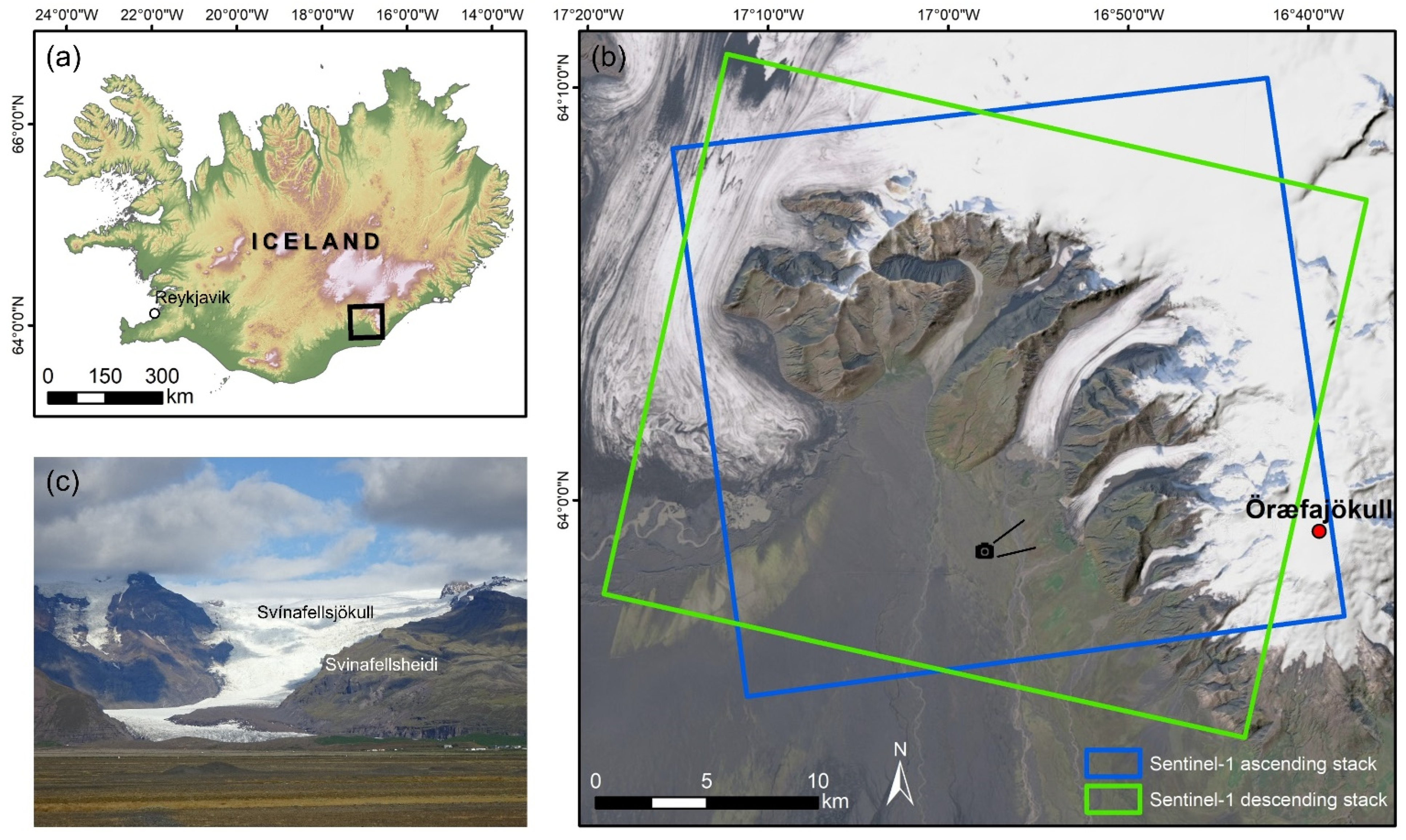
2.1. Study Area
2.2. Data
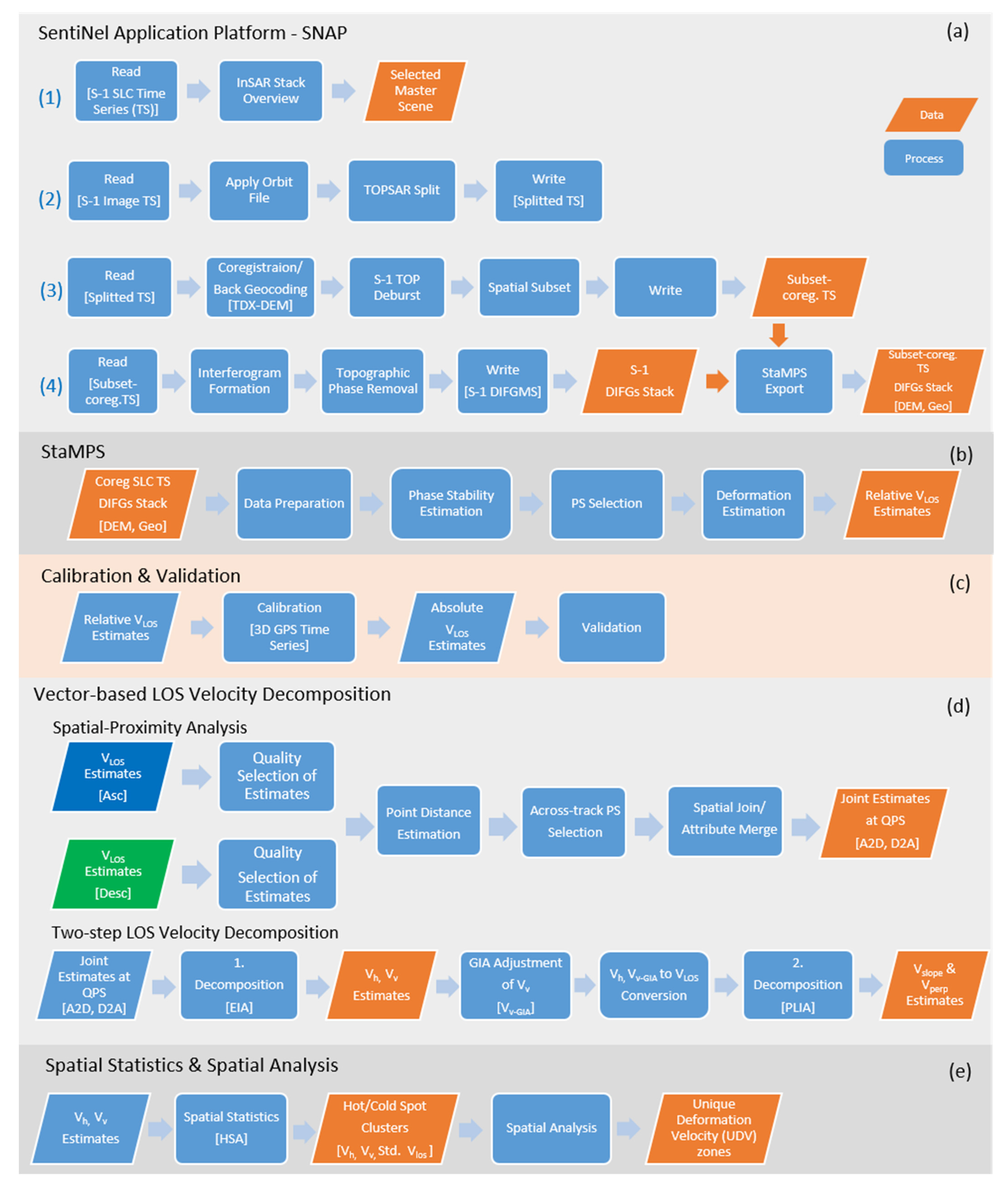
2.3. Methods
2.3.1. PSI Analysis for Deriving LOS Deformation Estimates
- Data Preparation, which involves selection of the initial PS Candidates (PSC) and processed-area subsetting (patches).
- Phase Stability Estimation, which includes phase noise estimation for each PSC in every interferogram. Gamma ( a coherence-like measure, is used to express the phase noise level of a PSC and its possibility to become a PS.
- PS Selection, which determines whether a PSC will be a PS based on their phase noise estimates. Only PSCs with persistent phase stability for the entire period were selected.
- Displacement/Deformation Estimation, which involves deformation signal isolation at PS pixel. This is achieved by unwrapping phase values and by subtracting various unwanted terms.
Calibration and Validation of LOS Estimates
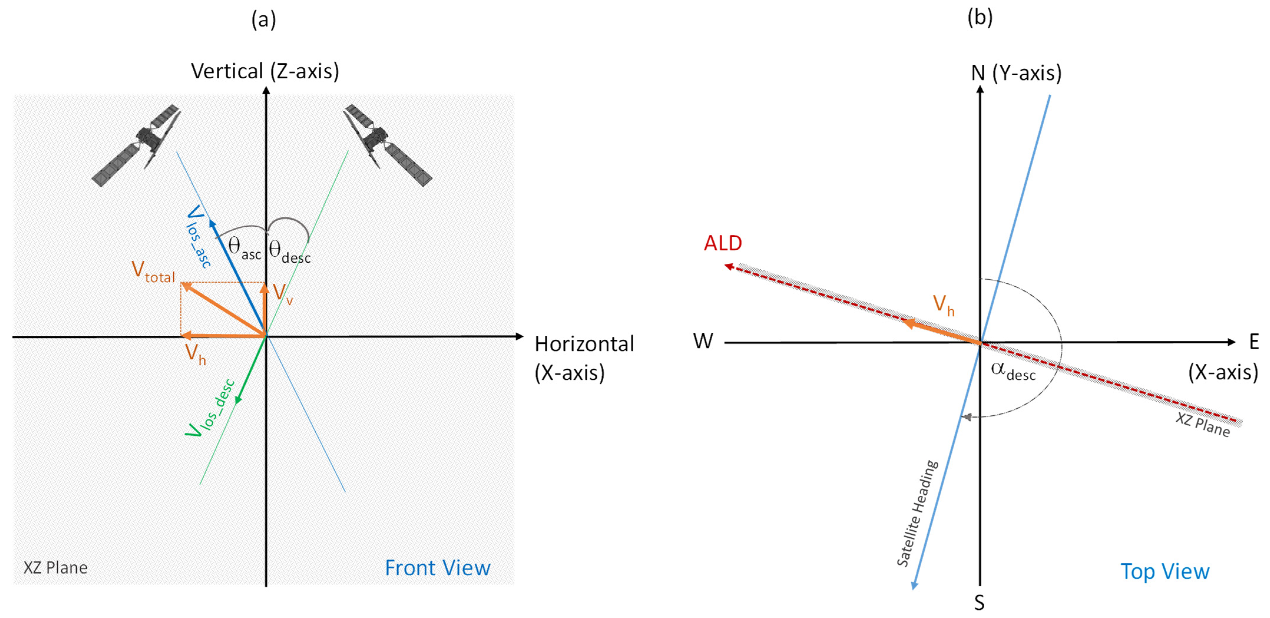
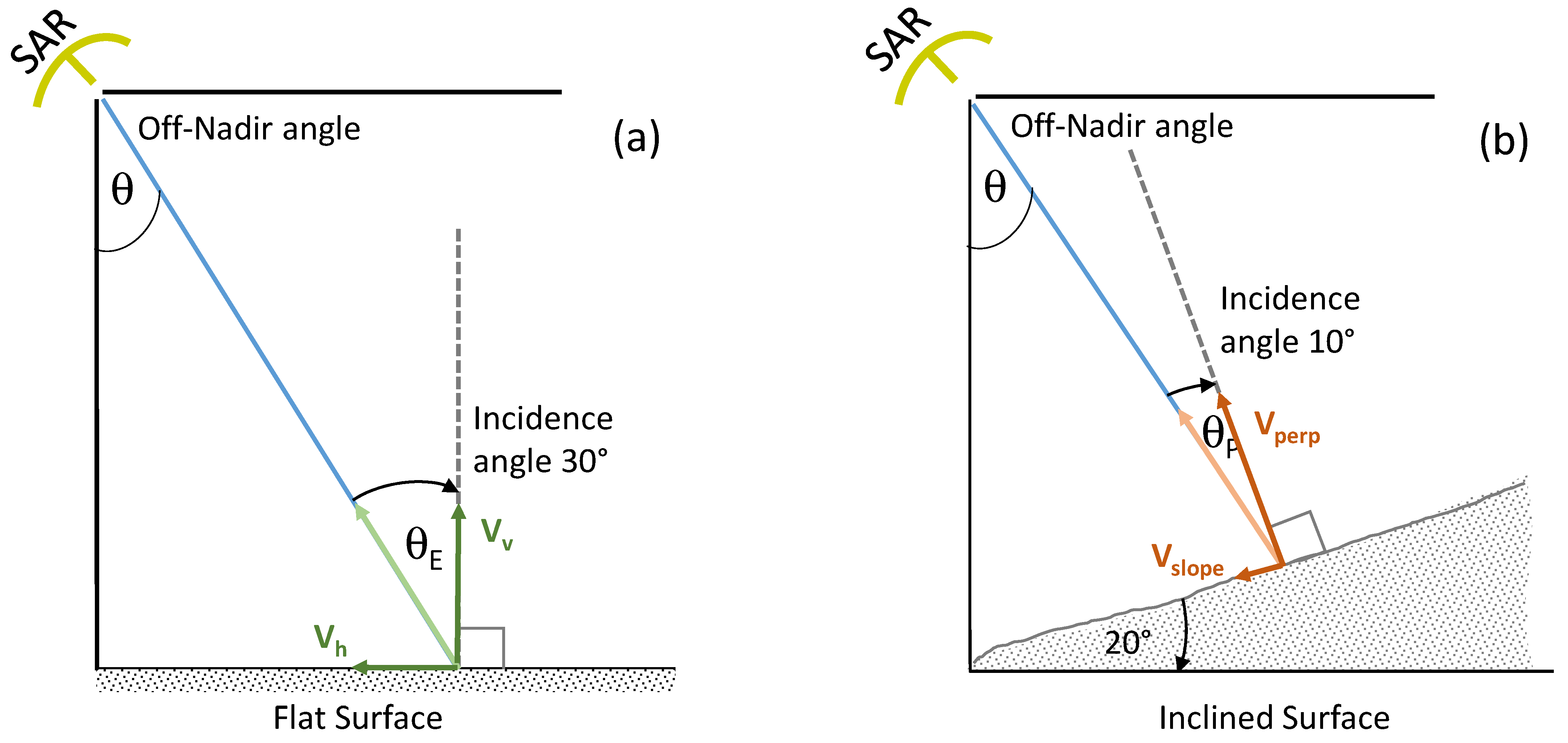
2.3.2. Decomposition of LOS Deformation Rate Estimates
Spatial-Proximity Analysis
Two-Step LOS Velocity Decomposition
2.3.3. Inferring the Local Deformation Fields Based on the PS-Based Estimates
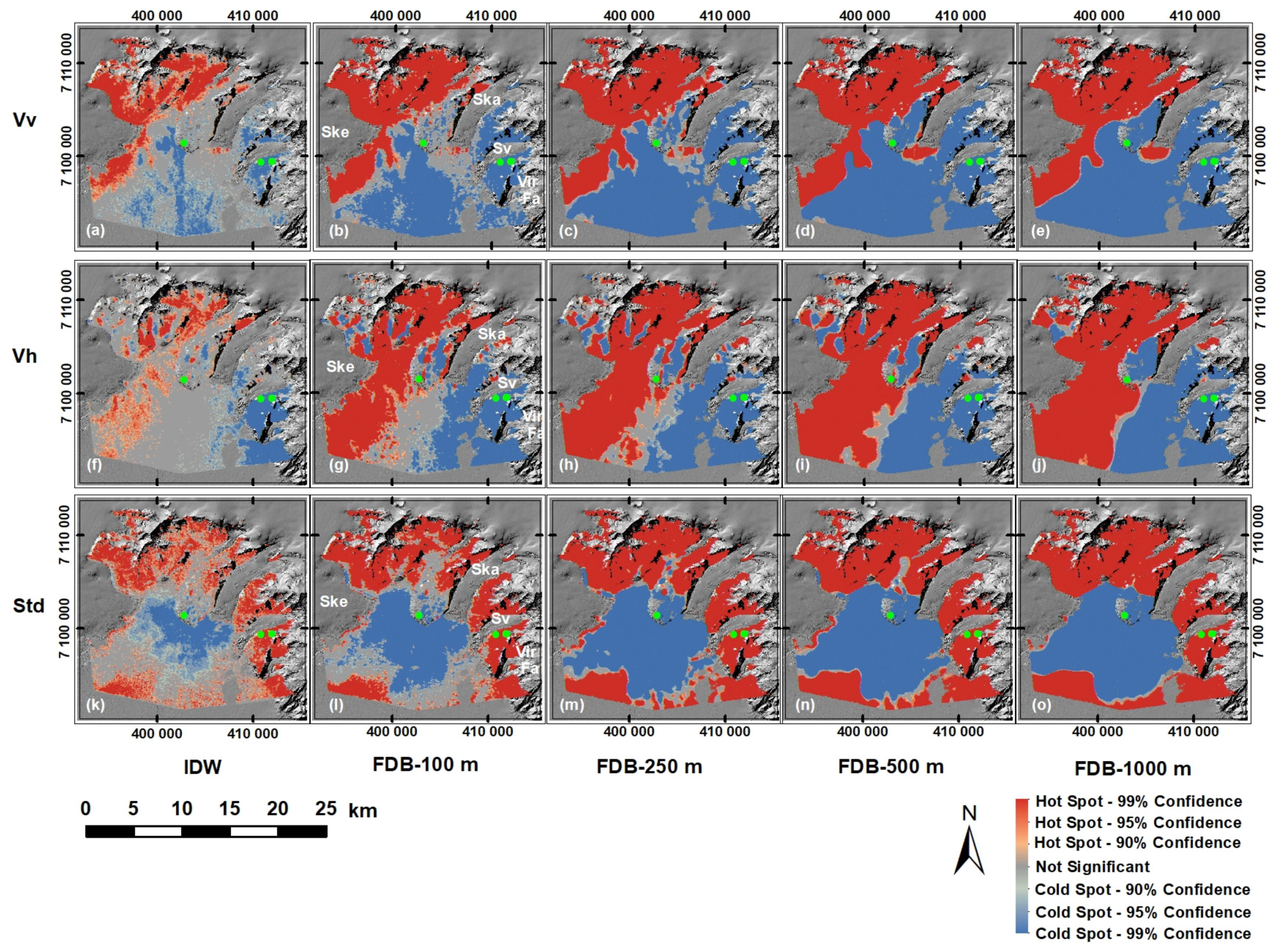
- The Calculate Distance Band tool was used to initially investigate the neighbourhood of PS estimates, i.e., the relationship between the number of neighbouring PS points and the spatial distance between them was assessed. By inputting the expected number of neighbouring points, required for an arbitrary PS, the average, the minimum and the maximum distance bands were estimated. The average distance in which one obtains a sufficient number of PSs (>30), was then used for HSA.
- Hot-Spot Analysis was applied to evaluate the spatial distribution of three relevant deformation parameters () based on two spatial relationship concepts, the Inverse Distance Weighted (IDW) and the Fixed Distance Band (FDB), at different spatial scales. By increasing the FDB distance from 100, 250, and 500 to 1000 m, Hot-Spot and Cold-Spot clusters in the AoI, ranging from fine (local) to coarser scales, were mapped.
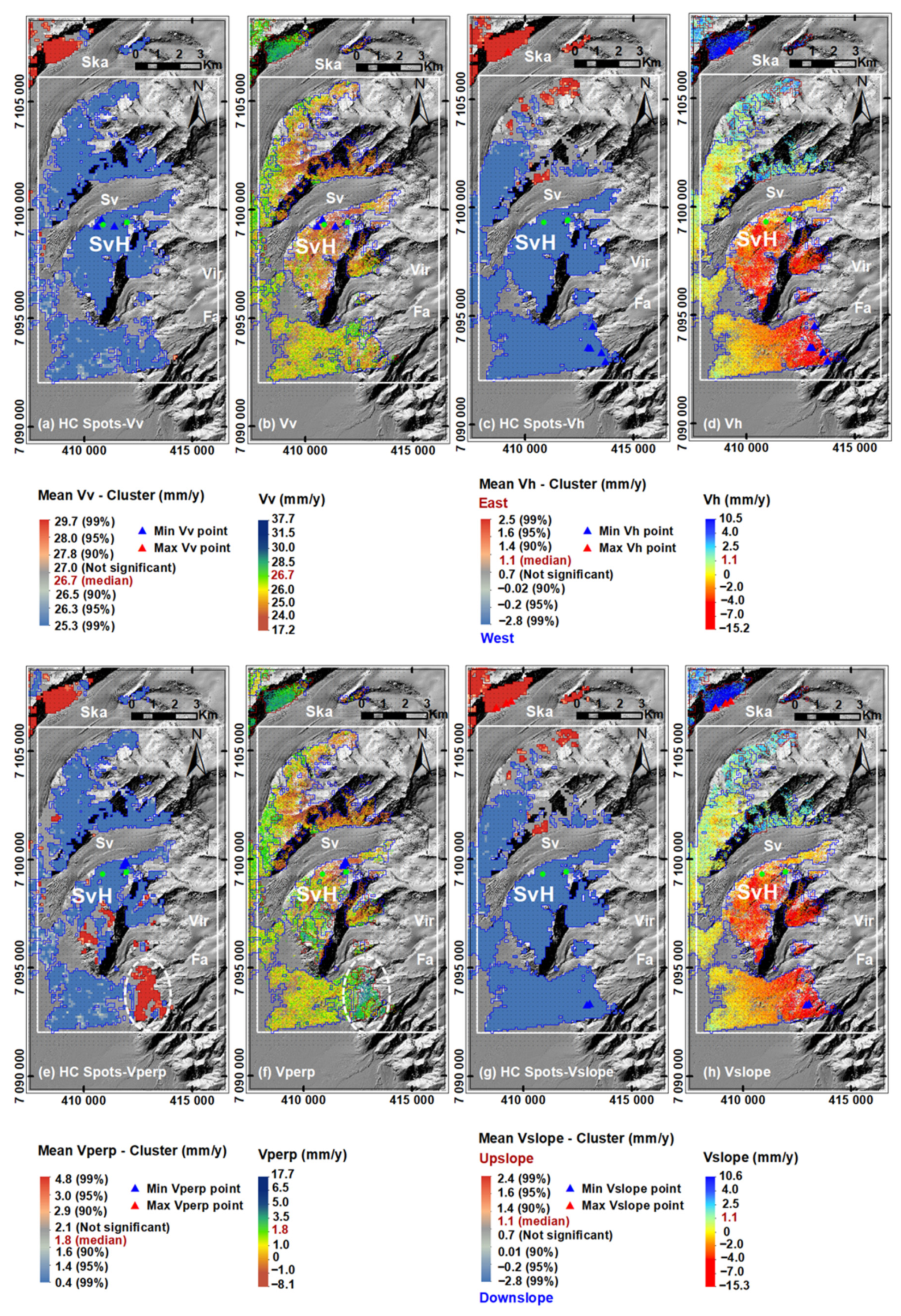
- The inputs for the spatial analysis were three rasterised deformation clusters from the HSA. To ensure high quality of the results, we selected three clusters (Hot Spot, Cold Spot, and not significant) with the highest confidence level (99%) of each parameter, resulting in nine distinct surface-deformation zones from each analysis.
3. Results
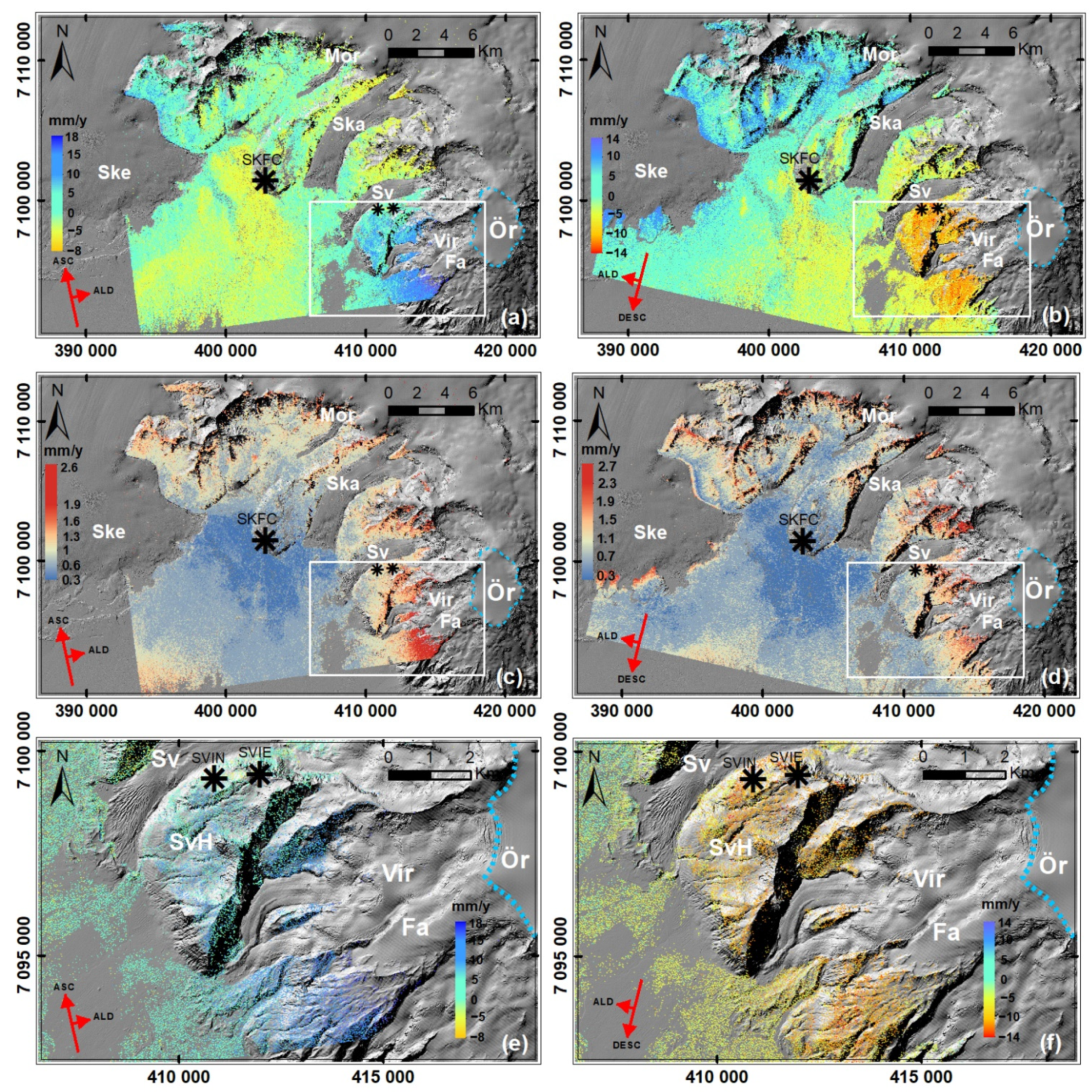
3.1. PS LOS Deformation-Rate Estimates
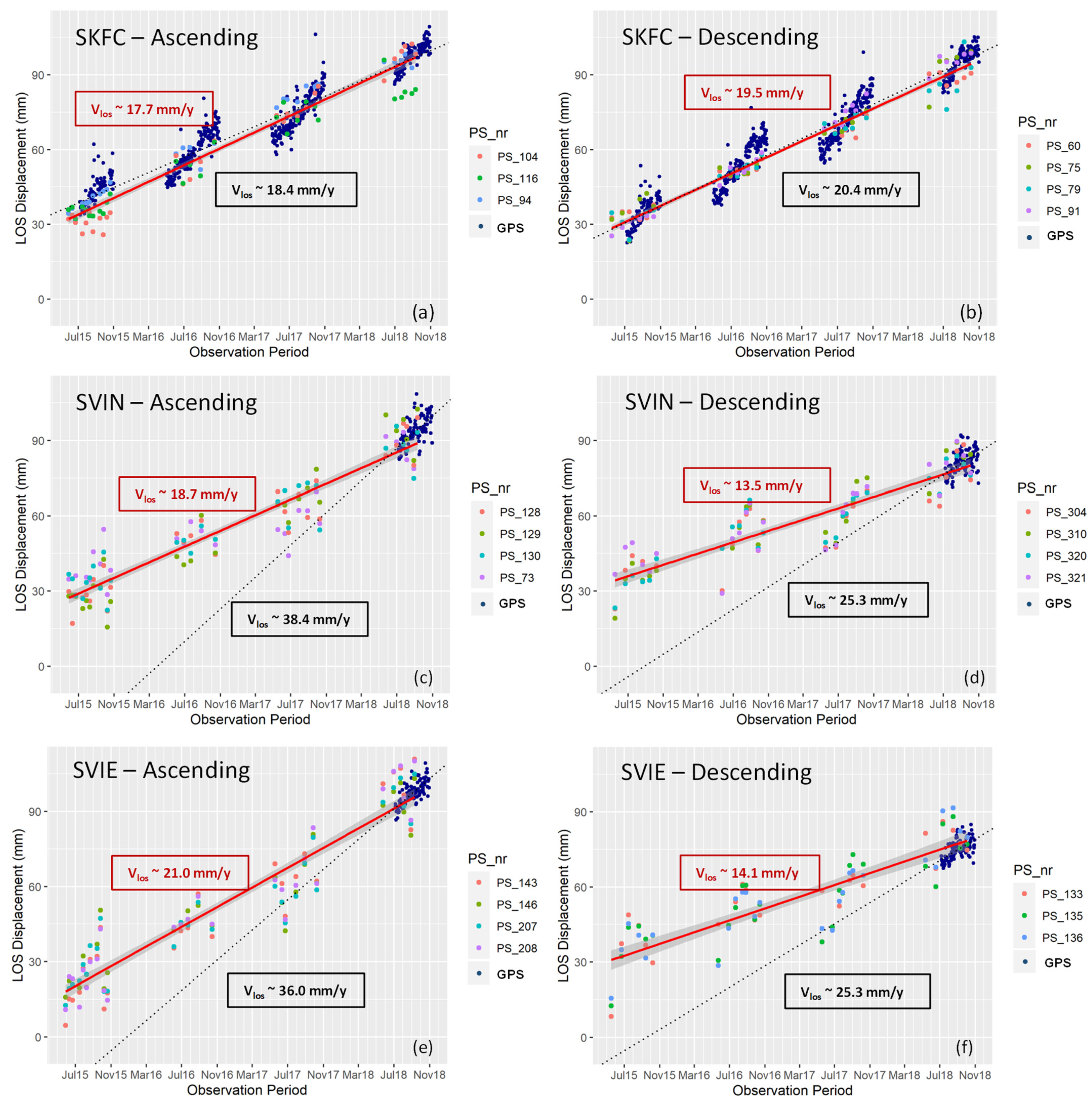
Validation of PS LOS Deformation-Rate Estimates
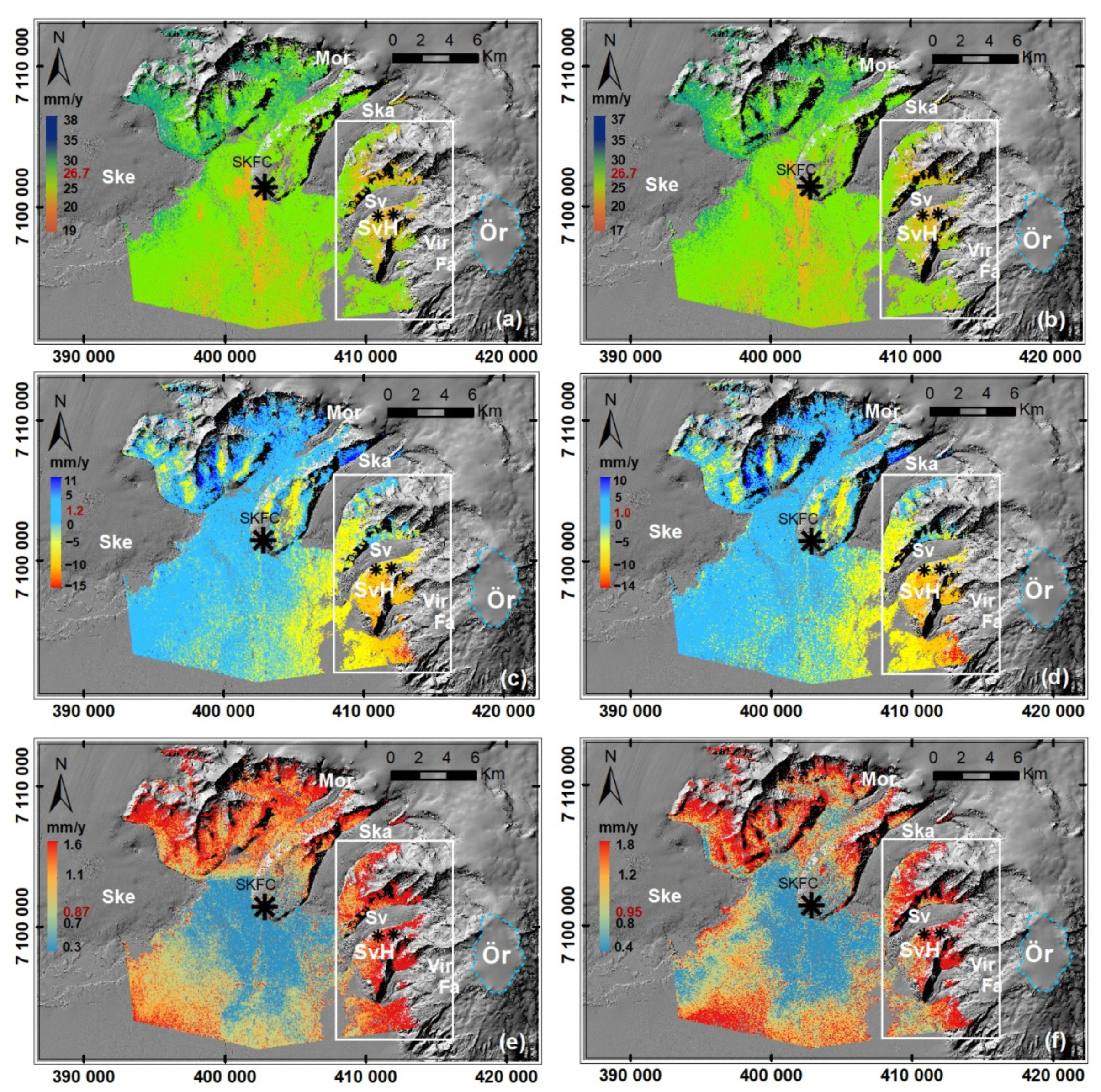
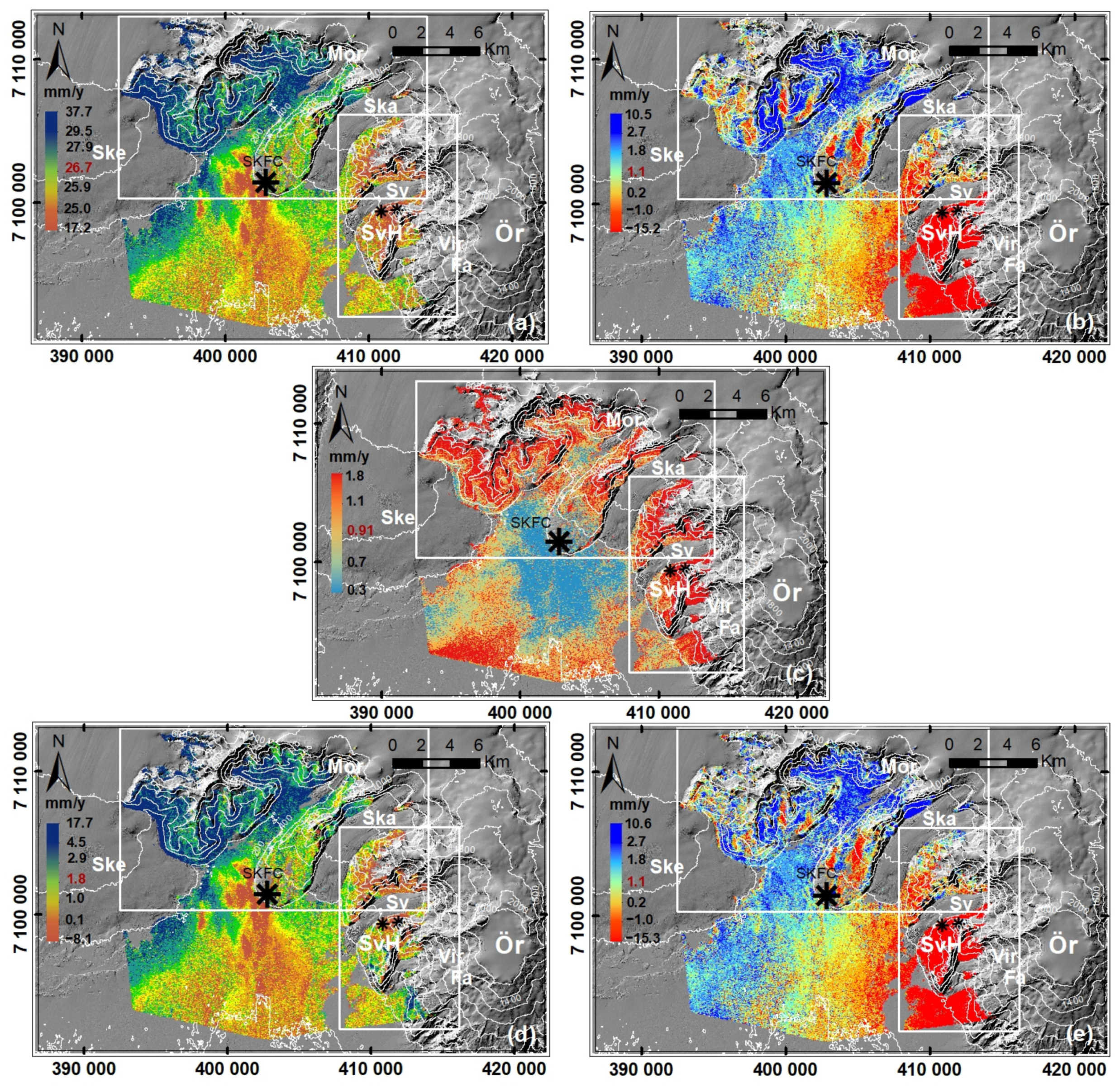
3.2. Two-Dimensional Decomposed Deformation Velocities
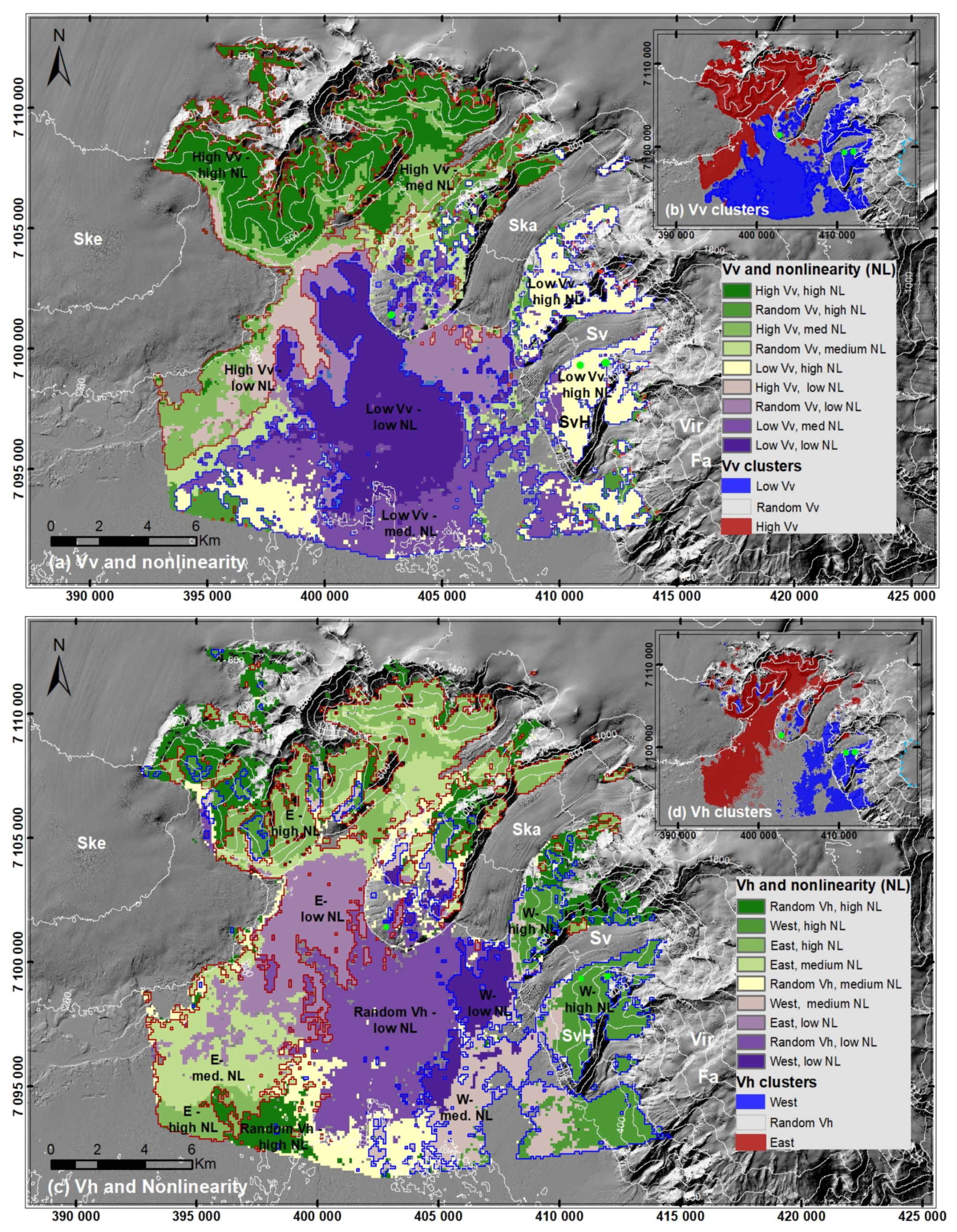
3.3. Derived Two-Dimensional Local Deformation Fields
3.3.1. Hot-Spot Analysis (HSA) Results
3.3.2. Interpretation of the Local Deformation Fields
4. Discussion
5. Conclusions
Author Contributions
Funding
Data Availability Statement
Acknowledgments
Conflicts of Interest
Appendix A. Decomposition Sensitivity

| Mission | Incidence Angle (Mid-Range) | East (E) | North (N) | Up (U) |
|---|---|---|---|---|
| Sentinel-1 (A) | 37° | −0.58 | −0.16 | 0.80 |
| Sentinel-1 (D) | 37° | 0.59 | −0.10 | 0.80 |
| Sentinel-1 (A) 1 | 43.4° | −0.68 | −0.11 | 0.73 |
| Sentinel-1 (D) 2 | 38.7° | 0.61 | −0.12 | 0.78 |
| TerraSAR-X (D) | 32° | 0.53 | −0.05 | 0.85 |
| ERS-1/2 (D) | 23° | 0.37 | −0.14 | 0.92 |
References
- Gabriel, A.K.; Goldstein, R.M.; Zebker, H.A. Mapping small elevation changes over large areas: Differential radar interferometry. J. Geophys. Res. 1989, 94, 9183–9191. [Google Scholar] [CrossRef]
- Ferretti, A.; Prati, C.; Rocca, F. Permanent scatterers in SAR interferometry. IEEE Trans. Geosci. Remote Sens. 2001, 39, 8–20. [Google Scholar] [CrossRef]
- Colesanti, C.; Wasowski, J. Investigating landslides with space-borne Synthetic Aperture Radar (SAR) interferometry. Eng. Geol. 2006, 88, 173–199. [Google Scholar] [CrossRef]
- Ferretti, A.; Prati, C.; Borghi, A.; Novali, F.; Savio, G.; Musazzi, S.; Barzaghi, R.; Rocca, F. Submillimeter Accuracy of InSAR Time Series: Experimental Validation. IEEE Trans. Geosci. Remote Sens. 2007, 45, 1142–1153. [Google Scholar] [CrossRef]
- Hooper, A.; Segall, P.; Zebker, H. Persistent scatterer interferometric synthetic aperture radar for crustal deformation analysis, with application to Volcán Alcedo, Galápagos. J. Geophys. Res. Solid Earth 2007, 112, 1–21. [Google Scholar] [CrossRef] [Green Version]
- Atzori, S.; Antonioli, A.; Tolomei, C.; de Novellis, V.; de Luca, C.; Monterroso, F. InSAR full-resolution analysis of the 2017–2018 M > 6 earthquakes in Mexico. Remote Sens. Environ. 2019, 234, 111461. [Google Scholar] [CrossRef]
- Albino, F.; Biggs, J.; Yu, C.; Li, Z. Automated Methods for Detecting Volcanic Deformation Using Sentinel-1 InSAR Time Series Illustrated by the 2017–2018 Unrest at Agung, Indonesia. J. Geophys. Res. Solid Earth 2020, 125, e2019JB017908. [Google Scholar] [CrossRef] [Green Version]
- Colesanti, C.; Ferretti, A.; Prati, C.; Rocca, F. Monitoring landslides and tectonic motions with the Permanent Scatterers Technique. Eng. Geol. 2003, 68, 3–14. [Google Scholar] [CrossRef]
- Bovenga, F.; Nitti, D.O.; Fornaro, G.; Radicioni, F.; Stoppini, A.; Brigante, R. Using C/X-band SAR interferometry and GNSS measurements for the Assisi landslide analysis. Int. J. Remote Sens. 2013, 34, 4083–4104. [Google Scholar] [CrossRef]
- Intrieri, E.; Raspini, F.; Fumagalli, A.; Lu, P.; del Conte, S.; Farina, P.; Allievi, J.; Ferretti, A.; Casagli, N. The Maoxian landslide as seen from space: Detecting precursors of failure with Sentinel-1 data. Landslides 2018, 15, 123–133. [Google Scholar] [CrossRef] [Green Version]
- Lauknes, T.R.; Piyush Shanker, A.; Dehls, J.F.; Zebker, H.A.; Henderson, I.H.C.; Larsen, Y. Detailed rockslide mapping in northern Norway with small baseline and persistent scatterer interferometric SAR time series methods. Remote Sens. Environ. 2010, 114, 2097–2109. [Google Scholar] [CrossRef]
- Worawattanamateekul, J.; Hoffmann, J.; Bamler, R.; Altermann, W.; Kampes, B.; Adam, N.; Roth, A. Derivation of Surface Subsidence Information in Bangkok (Thailand) by PS Analysis of a Limited Number of Interferograms. In Proceedings of the Fringe Workshop, Frascati, Italy, 28 November–2 December 2005. [Google Scholar]
- Yu, L.; Yang, T.; Zhao, Q.; Liu, M.; Pepe, A. The 2015–2016 ground displacements of the Shanghai coastal area inferred from a combined COSMO-SkyMed/Sentinel-1 DInSAR analysis. Remote Sens. 2017, 9, 1194. [Google Scholar] [CrossRef] [Green Version]
- Carlà, T.; Farina, P.; Intrieri, E.; Ketizmen, H.; Casagli, N. Integration of ground-based radar and satellite InSAR data for the analysis of an unexpected slope failure in an open-pit mine. Eng. Geol. 2018, 235, 39–52. [Google Scholar] [CrossRef]
- Ferretti, A.; Prati, C.; Rocca, F. Nonlinear subsidence rate estimation using permanent scatterers in differential SAR interferometry. IEEE Trans. Geosci. Remote Sens. 2000, 38, 2202–2212. [Google Scholar] [CrossRef] [Green Version]
- Bamler, R.; Eineder, M.; Adam, N.; Zhu, X.; Gernhardt, S. Interferometric potential of high resolution spaceborne SAR. Photogramm. Fernerkund. Geoinf. 2009, 2009, 407–419. [Google Scholar] [CrossRef]
- Crosetto, M.; Monserrat, O.; Cuevas-González, M.; Devanthéry, N.; Luzi, G.; Crippa, B. Measuring thermal expansion using X-band persistent scatterer interferometry. ISPRS J. Photogramm. Remote Sens. 2015, 100, 84–91. [Google Scholar] [CrossRef] [Green Version]
- Dong, J.; Zhang, L.; Tang, M.; Liao, M.; Xu, Q.; Gong, J.; Ao, M. Mapping landslide surface displacements with time series SAR interferometry by combining persistent and distributed scatterers: A case study of Jiaju landslide in Danba, China. Remote Sens. Environ. 2018, 205, 180–198. [Google Scholar] [CrossRef]
- ESA—Sentinel-1 Operations. Available online: https://www.esa.int/Enabling_Support/Operations/Sentinel-1_operations (accessed on 26 July 2021).
- Sentinel-1—Missions—Sentinel Online—Sentinel Online. Available online: https://sentinels.copernicus.eu/web/sentinel/missions/sentinel-1 (accessed on 26 July 2021).
- SNAP—STEP. Available online: https://step.esa.int/main/toolboxes/snap/ (accessed on 26 July 2021).
- Veci, L.; Prats-Iraola, P.; Scheiber, R.; Collard, F.; Fomferra, N.; Engdahl, M. The Sentinel-1 Toolbox. In Proceedings of the IEEE International Geoscience and Remote Sensing Symposium (IGARSS), Québec, QC, Canada, 13–18 July 2014; pp. 1–3. [Google Scholar]
- Wasowski, J.; Bovenga, F. Investigating landslides and unstable slopes with satellite Multi Temporal Interferometry: Current issues and future perspectives. Eng. Geol. 2014, 174, 103–138. [Google Scholar] [CrossRef]
- Bianchini, S.; Cigna, F.; Righini, G.; Proietti, C.; Casagli, N. Landslide HotSpot Mapping by means of Persistent Scatterer Interferometry. Environ. Earth Sci. 2012, 67, 1155–1172. [Google Scholar] [CrossRef]
- Solari, L.; Del Soldato, M.; Montalti, R.; Bianchini, S.; Raspini, F.; Thuegaz, P.; Bertolo, D.; Tofani, V.; Casagli, N. A Sentinel-1 based hot-spot analysis: Landslide mapping in north-western Italy. Int. J. Remote Sens. 2019, 40, 7898–7921. [Google Scholar] [CrossRef]
- Confuorto, P.; Di Martire, D.; Centolanza, G.; Iglesias, R.; Mallorqui, J.J.; Novellino, A.; Plank, S.; Ramondini, M.; Thuro, K.; Calcaterra, D. Post-failure evolution analysis of a rainfall-triggered landslide by multi-temporal interferometry SAR approaches integrated with geotechnical analysis. Remote Sens. Environ. 2017, 188, 51–72. [Google Scholar] [CrossRef]
- Lu, P.; Casagli, N.; Catani, F.; Tofani, V. Persistent scatterers interferometry hotspot and cluster analysis (PSI-HCA) for detection of extremely slow-moving landslides. Int. J. Remote Sens. 2012, 33, 466–489. [Google Scholar] [CrossRef]
- Dai, K.; Li, Z.; Tomás, R.; Liu, G.; Yu, B.; Wang, X.; Cheng, H.; Chen, J.; Stockamp, J. Monitoring activity at the Daguangbao mega-landslide (China) using Sentinel-1 TOPS time series interferometry. Remote Sens. Environ. 2016, 186, 501–513. [Google Scholar] [CrossRef] [Green Version]
- Carlà, T.; Intrieri, E.; Raspini, F.; Bardi, F.; Farina, P.; Ferretti, A.; Colombo, D.; Novali, F.; Casagli, N. Perspectives on the prediction of catastrophic slope failures from satellite InSAR. Sci. Rep. 2019, 9, 14137. [Google Scholar] [CrossRef] [Green Version]
- Adam, N.; Kampes, B.M.; Eineder, M.; Worawattanamateekul, J.; Kircher, M. The development of a scientific permanent scatterer system. In Proceedings of the Joint ISPRS/EARSeL Workshop “High Resolution Mapping from Space”, Hannover, Germany, 6–8 October 2003. [Google Scholar]
- Kampes, B.M. Radar Interferometry Persistent Scatterer Technique; Springer: Dordrecht, The Netherlands, 2006; ISBN 9781402045769. [Google Scholar]
- Hooper, A. A multi-temporal InSAR method incorporating both persistent scatterer and small baseline approaches. Geophys. Res. Lett. 2008, 35, 1–5. [Google Scholar] [CrossRef] [Green Version]
- Árnadóttir, T.; Lund, B.; Jiang, W.; Geirsson, H.; Björnsson, H.; Einarsson, P.; Sigurdsson, T. Glacial rebound and plate spreading: Results from the first countrywide GPS observations in Iceland. Geophys. J. Int. 2009, 177, 691–716. [Google Scholar] [CrossRef] [Green Version]
- Auriac, A.; Spaans, K.H.; Sigmundsson, F.; Hooper, A.; Schmidt, P.; Lund, B. Iceland rising: Solid Earth response to ice retreat inferred from satellite radar interferometry and visocelastic modeling. J. Geophys. Res. Solid Earth 2013, 118, 1331–1344. [Google Scholar] [CrossRef] [Green Version]
- Drouin, V.; Sigmundsson, F. Countrywide Observations of Plate Spreading and Glacial Isostatic Adjustment in Iceland Inferred by Sentinel-1 Radar Interferometry, 2015–2018. Geophys. Res. Lett. 2019, 46, 8046–8055. [Google Scholar] [CrossRef]
- Rocca, F. 3D motion recovery with multi-angle and/or left right interferometry. In Proceedings of the Fringe 2003 Workshop, Frascati, Italy, 1–5 December 2003. [Google Scholar]
- Wright, T.J. Toward mapping surface deformation in three dimensions using InSAR. Geophys. Res. Lett. 2004, 31, L01607. [Google Scholar] [CrossRef] [Green Version]
- Helgason, J.; Duncan, R.A. Stratigraphy, 40Ar-39Ar dating and erosional history of Svínafell, SE Iceland. Jökull 2013, 63, 33–53. [Google Scholar]
- Sæmundsson, Þ.; Sigurðsson, I.A.; Pétursson, H.G.; Jónsson, H.P.; Decaulne, A.; Roberts, M.J.; Jensen, E.H. Bergflóðið sem féll á Morsárjökul 20. mars 2007—Hverjar hafa afleiðingar þess orðið? Náttúrufræðingurinn 2011, 81, 131–141. [Google Scholar]
- Ben-Yehoshua, D.; Sæmundsson, Þ.; Helgason, J.K.; Belart, J.M.C.; Sigurðsson, J.V.; Erlingsson, S. Paraglacial exposure and collapse of glacial sediment: The 2013 landslide onto Svínafellsjökull, southeast Iceland. Earth Surf. Process. Landf. 2022. [Google Scholar] [CrossRef]
- Sigmundsson, F.; Einarsson, P.; Hjartardóttir, Á.R.; Drouin, V.; Jónsdóttir, K.; Árnadóttir, T.; Geirsson, H.; Hreinsdóttir, S.; Li, S.; Ófeigsson, B.G. Geodynamics of Iceland and the signatures of plate spreading. J. Volcanol. Geotherm. Res. 2018, 391, 106436. [Google Scholar] [CrossRef]
- ArcticDEM—Polar Geospatial Center. Available online: https://www.pgc.umn.edu/data/arcticdem/ (accessed on 27 July 2021).
- German Aerospace Center. DEM Products Specification Document (Doc: TD-GS-PS-0021); Issue 3.0; German Aerospace Center: Wessling, Germany, 2013. [Google Scholar]
- de Zan, F.; Guarnieri, A.M. TOPSAR: Terrain observation by progressive scans. IEEE Trans. Geosci. Remote Sens. 2006, 44, 2352–2360. [Google Scholar] [CrossRef]
- Foumelis, M.; Blasco, J.M.D.; Desnos, Y.L.; Engdahl, M.; Fernández, D.; Veci, L.; Lu, J.; Wong, C. ESA SNAP—Stamps integrated processing for Sentinel-1 persistent scatterer interferometry. In Proceedings of the International Geoscience and Remote Sensing Symposium (IGARSS), Valencia, Spain, 22–27 July 2018; Volume 2018. [Google Scholar]
- Hooper, A.; Bekaert, D.; Spaans, K.; Arikan, M. Recent advances in SAR interferometry time series analysis for measuring crustal deformation. Tectonophysics 2012, 514–517, 1–13. [Google Scholar] [CrossRef]
- Hooper, A.; Spaans, K.; Bekaert, D.; Cuenca, M.C.; Arıkan, M. StaMPS/MTI Manual Version 4.1b. 2018, p. 44. Available online: https://docplayer.net/94667136-Stamps-mti-manual-version-4-1b-andy-hooper-david-bekaert-ekbal-hussain-and-karsten-spaans-15th-august-2018.html (accessed on 5 April 2022).
- Foumelis, M. Vector-based approach for combining ascending and descending persistent scatterers interferometric point measurements. Geocarto Int. 2018, 33, 38–52. [Google Scholar] [CrossRef]
- Hanssen, R.F. Radar Interferometry: Data Interpretation and Error Analysis; Kluwer Academic Publishers: Dordrecht, The Netherlands, 2001; ISBN 0-7923-6945-9. [Google Scholar]
- Fuhrmann, T.; Garthwaite, M.C. Resolving three-dimensional surface motion with InSAR: Constraints from multi-geometry data fusion. Remote Sens. 2019, 11, 241. [Google Scholar] [CrossRef] [Green Version]
- Blasco, J.M.D.; Foumelis, M.; Stewart, C.; Hooper, A. Measuring urban subsidence in the Rome Metropolitan Area (Italy) with Sentinel-1 SNAP-StaMPS Persistent Scatterer Interferometry. Remote Sens. 2019, 11, 129. [Google Scholar] [CrossRef] [Green Version]
- Sigmundsson, F.; Parks, M.; Pedersen, R.; Jónsdóttir, K.; Ófeigsson, B.G.; Grapenthin, R.; Dumont, S.; Einarsson, P.; Drouin, V.; Rafn Heimisson, E.; et al. Magma movements in volcanic plumbing systems and their associated ground deformation and seismic patterns. In Volcanic and Igneous Plumbing Systems: Understanding Magma Transport, Storage, and Evolution in the Earth’s Crust; Elsevier Inc.: Amsterdam, The Netherlands, 2018; pp. 285–322. ISBN 9780128097496. [Google Scholar]
- Drouin, V.; Heki, K.; Sigmundsson, F.; Hreinsdóttir, S.; Ófeigsson, B.G. Constraints on seasonal load variations and regional rigidity from continuous GPS measurements in Iceland, 1997–2014. Geophys. J. Int. 2016, 205, 1843–1858. [Google Scholar] [CrossRef] [Green Version]
- ArcGIS Desktop 10.7.1 Quick Start Guide—ArcMap|Documentation. Available online: https://desktop.arcgis.com/en/arcmap/10.7/get-started/setup/arcgis-desktop-quick-start-guide.htm (accessed on 27 July 2021).
- Equilibrium Line|Vatnajokull National Park. Available online: https://www.vatnajokulsthjodgardur.is/en/areas/melting-glaciers/glaciology/equilibrium-line (accessed on 2 August 2021).
- Gudmundsson, S.; Sigmundsson, F.; Carstensen, J.M. Three-dimensional surface motion maps estimated from combined interferometric synthetic aperture radar and GPS data. J. Geophys. Res. Solid Earth 2002, 107, ETG 13-1–ETG 13-14. [Google Scholar] [CrossRef]
- Gernhardt, S.M. High Precision 3D Localization and Motion Analysis of Persistent Scatterers Using Meter-Resolution Radar Satellite Data. Ph.D. Thesis, Technical University of Munich, Munich, Germany, 2011. [Google Scholar]

| Data | Resolution (m) | Description |
|---|---|---|
| Sentinel-1 SAR | 2.3 × 14.1 1 | Orbit: Ascending (A118) Acquisition time: 29/05/2015–10/09/2018 No. of ifgs 3: 28 Incidence angle (EIA): 41.2°–45.6° Heading: 350.6° |
| Sentinel-1 SAR | 2.3 × 14.1 2 | Orbit: Descending (D111) Acquisition time: 17/05/2015–04/10/2018 No. of ifgs: 25 Incidence angle (EIA): 36.0°–41.5° Heading: 191.0° |
| Arctic-DEM | 2 | Derived from stereo–optical imagery acquired during 2012–2017 |
| Tandem-X DEM | 20 | Derived from radar imagery acquired during 2011–2015 |
| GPS deformation time-series 4 SKFC 5 SVIN SVIE | Observation period: July 2015–October 2018 July 2018–October 2018 July 2018–October 2018 |
| Pass/Orbit | Master Scene (# of ifg) | Nr. of PS (PS/km2) | |||
|---|---|---|---|---|---|
| A118 | 27/08/2016 (28 ifgs) | 214,061 (~460) | −8.1 to +17.9 (0.3) | 10.3 to 36.3 (18.7) | 0.3 to 2.6 (0.9) |
| D111 | 26/09/2016 (25 ifgs) | 228,335 (~480) | −13.7 to +13.6 (0.6) | 6.7 to 34.0 (21.1) | 0.3 to 2.7 (1.0) |
| Station (# GPS Obs.) | GPS dN 1/sN 2 (mm) | GPS dE/sE (mm) | GPS dU/sU (mm) | Data | ||
|---|---|---|---|---|---|---|
| SKFC (550) | −13.0/2.6 | 6.1/2.1 | 45.8/8.0 | A D | 18.4/19.7 20.4/19.5 | 0.5–1.0 0.4–1.1 |
| SVIN (109) | −2.8/2.1 | −2.4/1.8 | 9.3/6.8 | A D | 38.4/18.7 25.3/13.5 | 1.1–1.4 1.1–1.4 |
| SVIE (107) | −3.0/2.0 | −2.1/1.7 | 7.7/6.3 | A D | 36.0/21.0 25.3/14.1 | 1.4–1.6 1.6–1.8 |
| Dataset | QPS 2 Density PS/km2 | # Across-Track 3 PSs Min. to Max. (Mean) | ||
|---|---|---|---|---|
| A2D | ~396 | 1–47 (17) | −18.9 to 37.7 (26.7) | −15.2 to 10.5 (1.2) |
| D2A | ~360 | 1–39 (17) | −17.2 to 37.1 (26.7) | −14.4 to 9.5 (1.0) |
| Combined 1 1st decomposition | ~757 | −17.2 to 37.7 (26.7) | −15.2 to 10.5 (1.1) | |
| Combined (after GIA-SS removal) | ~757 | −7.8 to 12.7 (1.7) | −15.2 to 10.5 (1.1) | |
| Combined 2nd decomposition | ~757 | −8.1 to 17.7 (1.8) | −15.3 to 10.6 (1.1) |
Publisher’s Note: MDPI stays neutral with regard to jurisdictional claims in published maps and institutional affiliations. |
© 2022 by the authors. Licensee MDPI, Basel, Switzerland. This article is an open access article distributed under the terms and conditions of the Creative Commons Attribution (CC BY) license (https://creativecommons.org/licenses/by/4.0/).
Share and Cite
Dittrich, J.; Hölbling, D.; Tiede, D.; Sæmundsson, Þ. Inferring 2D Local Surface-Deformation Velocities Based on PSI Analysis of Sentinel-1 Data: A Case Study of Öræfajökull, Iceland. Remote Sens. 2022, 14, 3166. https://doi.org/10.3390/rs14133166
Dittrich J, Hölbling D, Tiede D, Sæmundsson Þ. Inferring 2D Local Surface-Deformation Velocities Based on PSI Analysis of Sentinel-1 Data: A Case Study of Öræfajökull, Iceland. Remote Sensing. 2022; 14(13):3166. https://doi.org/10.3390/rs14133166
Chicago/Turabian StyleDittrich, Jirathana, Daniel Hölbling, Dirk Tiede, and Þorsteinn Sæmundsson. 2022. "Inferring 2D Local Surface-Deformation Velocities Based on PSI Analysis of Sentinel-1 Data: A Case Study of Öræfajökull, Iceland" Remote Sensing 14, no. 13: 3166. https://doi.org/10.3390/rs14133166
APA StyleDittrich, J., Hölbling, D., Tiede, D., & Sæmundsson, Þ. (2022). Inferring 2D Local Surface-Deformation Velocities Based on PSI Analysis of Sentinel-1 Data: A Case Study of Öræfajökull, Iceland. Remote Sensing, 14(13), 3166. https://doi.org/10.3390/rs14133166