Abstract
Remotely sensed vegetation indices have been widely used to estimate live fuel moisture content (LFMC). However, marked differences in vegetation structure affect the relationship between field-measured LFMC and reflectance, which limits spatial extrapolation of these indices. To overcome this limitation, we explored the potential of random forests (RF) to estimate LFMC at the subcontinental scale in the Mediterranean basin wildland. We built RF models (LFMCRF) using a combination of MODIS spectral bands, vegetation indices, surface temperature, and the day of year as predictors. We used the Globe-LFMC and the Catalan LFMC monitoring program databases as ground-truth samples (10,374 samples). LFMCRF was calibrated with samples collected between 2000 and 2014 and validated with samples from 2015 to 2019, with overall root mean square errors (RMSE) of 19.9% and 16.4%, respectively, which were lower than current approaches based on radiative transfer models (RMSE ~74–78%). We used our approach to generate a public database with weekly LFMC maps across the Mediterranean basin.
1. Introduction
Live fuel moisture content (LFMC), the mass of water in the foliage and small twigs relative to its total dry mass, is a key factor affecting fire potential and determining wildfire danger and activity [1,2]. Fuel moisture is directly related to the amount of energy needed to evaporate water before ignition [2,3]. Consequently, high moisture values reduce, or even inhibit, ignitability and subsequent fire spread [4].
Different studies conducted in a wide range of ecosystems have found a significant correlation between burned area and LFMC [5,6,7]. More specifically, these studies report that large fires only occur once fuel moisture crosses critical dryness levels. In Mediterranean regions, longer summer drought periods along with increases in temperature have been projected under climate change [8]. Such climatic changes could significantly decline LFMC and consequently enhance the length of the fire season and the rate of high intensity fires [9]. This situation could be exacerbated with intensifying fuel load accumulation and fuel connectivity as a result of rural exodus and widespread lack of land management. As a consequence, the probability and the frequency of extreme fire events is expected to increase [9]. Accurate and comprehensive spatial and temporal estimations of LFMC are thus needed to assess wildfire danger [10] and to develop early warning systems for the evolution of critical conditions [11].
Regional-scale assessment of LFMC is commonly obtained through expensive and time-consuming field inventories [12,13] or through meteorological drought indices (e.g., [14]). The latter allow spatially continuous measurements, but their validity for the Mediterranean areas has been questioned in various studies [15,16,17], as they do not take into account plant-specific differences and the influence of site conditions (e.g., soil water dynamics), often leading to poor predictions [3].
Remote sensing of LFMC using satellite information provides a valuable alternative to overcome the limitations of drought indices. Current approaches are mainly grouped into either physically-based simulation [18,19,20] or empirical methods [15,21,22,23]. Generally, these methods measure how water absorption and leaf properties affect reflectance in the optical spectrum [24]. Physical approaches, such as radiative transfer models (RTM), are expected to be more robust than empirical methods [10]. This is because they are based on the physical associations between leaf-canopy properties and spectral reflectance, which are independent of sensor and site conditions [19,25]. However, they are also more complex to parameterize and require additional ecological information and prior knowledge over large geographical gradients to prevent unrealistic spectra simulations [25]. In contrast, empirical approaches, which are commonly based on spectral indices (SI), are simpler and have shown similar or even better accuracies than physical models when applied locally [19,26] or across specific vegetation types [20].
Combinations of SI have been successfully employed to estimate LFMC [6,15,21,26]. In addition, some authors found stronger predictive power by including land surface temperature (LST) along with optical data to the empirical relationships [22,27,28,29]. The connection between LFMC and LST lies on the interaction between the plant energy balance mechanisms and its response to water stress [24]. Other recent studies implement microwave remote sensing to retrieve LFMC [30,31,32], but their use still has some limitations, such as data availability.
The application of empirical approaches at continental or global scales is precisely constrained by the availability of data for calibration during model development [18,21]. The biophysical and structural differences among species impact the functional relationships between LFMC and remotely sensed reflectance spectra [33,34]. Consequently, a large number of diverse sampling observations is required to reduce the effect of site dependence. Furthermore, the use of many predictive variables potentially related to LFMC may significantly improve the empirical estimations of the model [20], but also increase its complexity.
Machine learning (ML) algorithms, such as random forests (RF), are a solid alternative to physically based RTM methods or the classical regression models on which the empirical approaches are commonly based. ML algorithms are highly efficient with high dimensional data and solve the problem of model complexity by applying different functional forms in the relation between predictors and LFMC, without make explicit a priori assumptions [35]. However, using ML to estimate LFMC from remote sensing is still very recent [28,31,34,36] and has not been used in the Mediterranean basin.
Despite the importance of wildfires in the Mediterranean basin, we are currently lacking a specific method to reliably estimate LFMC at the subcontinental scale. For example, the European Forest Fires Information System (EFFIS) is using the Australian operational system [20] to estimate LFMC in the European extent, but this method has not been broadly assessed yet. Other studies have addressed LFMC modelling at local [26,37] or regional [18,25] scales and they are usually focused on specific vegetation types (e.g., grasslands or shrublands). Thus, we are still lacking a product that provides LFMC estimates for the Mediterranean basin. The only exception is the global LFMC product developed by Quan et al. [38], which is based on an RTM, and it is not yet known whether LFMC estimates could be improved through ML approaches.
The present study aims to fill this knowledge gap by developing an RF algorithm to predict LFMC within the Western Mediterranean basin using the information of the widely used Moderate Resolution Imaging Spectroradiometer (MODIS), and comparing the results with the only other method available for this area, the physically-based estimations of Quan et al. [38]. We also aim to generalize the model over a wide range of fuel types with a unique formulation by combining a forward feature selection with a spatial cross-validation and ML techniques. Finally, our ultimate goal is to develop a database of LFMC for the Mediterranean basin using available data that improves beyond currently existing products.
2. Materials and Methods
2.1. Data
2.1.1. LFMC Field Measurements
We used all the LFMC data publicly accessible within the Mediterranean basin. Most of the data available so far have been compiled in the Globe-LFMC database [39] (last accessed June 2021). The Globe-LFMC is a global compilation of 161,717 LFMC destructive field measurements of leaves and small twigs (<6 mm) from 1977 to 2018 at 1383 sampling sites with different species and characteristics in 11 fire-prone countries [39]. Most of the records in the study area come from The French Réseau hydrique database [13], but we also found a more recent LFMC time series from Catalonia (Cat-LFMC) [12]. This is a collection of 21 years (1998–2019) of biweekly field-sampled data compiled by the Catalan Forest Fire Prevention Service across nine sampling areas within this Spanish region, and focused on five species representatives of Mediterranean shrublands [12]. Cat-LFMC was added to the Globe-LFMC to extend the total number of sites and the time interval within the Mediterranean area. Both datasets have already been technically validated by correcting inconsistencies and anomalies in LFMC, as described in the relevant publications [12,13,39]. All records are properly georeferenced and inform about the species collected, the sampling protocol, land cover type, and further eco-physiological and environmental properties not used in this study. Cat-LFMC additionally includes a quality control flag, indicating possible outliers related to abrupt changes in LFMC values. These outliers were removed from the database prior to analyses.
2.1.2. MODIS Data
The MODIS MCD43A4 Collection 6 product [40] was selected as a source of aboveground spectral information, as it has shown good performance in previous studies [21,26,34]. MCD43A4 provides daily maps at 500 m spatial resolution from a 16-day composite of Nadir Bidirectional Distribution Function (NBDF)-Adjusted Reflectance for each of the 7 MODIS bands (channels 1–7, Table 1). Using a composite product may reduce the probability of cloud cover and shadows. The ‘Good quality’ flag from the simplified band specific quality layers (BRDF_Albedo_Band_Quality) associated with MCD43A4 was used to keep the full quality pixels of the composite.

Table 1.
List of potential predictors of LFMC.
The Terra MODIS Land Surface Temperature (LST) MOD11A2 Collection 6 product was included as a predictor of LFMC due to the impact of water availability in plant evapotranspiration and, consequently, on canopy temperature [24]. MOD11A2 is an 8-day pixel average from the MOD11A1, a daily product of LST measurements from the Terra satellite [41]. We used the daytime composite values, instead of single day measurements, because MOD11A2 had fewer data gaps (8% vs. 35%), and their effect on LFMC predictions, in terms of model RMSE, was the same (~20%, see Section S1). Daytime images cover the same period as MCD43A4, and they coincide better with the typical sample collection time, but at a 1000 m spatial resolution. They were resampled to the 500 m spatial resolution of MCD43A4 using a bilinear interpolation.
Additionally, the annual MODIS Land Cover Type (MCD12Q1) Collection 6 product [42] with the International Geosphere-Biosphere Programme (IGBP) classification scheme was used to distinguish between vegetation types in the analyses. This product replaced the land cover field included in the Globe-LFMC database, which is based on the ESA Climate Change Initiative Land Cover for the year 2015. This is because MCD12Q1 accommodates to the spatial resolution of the reflectance data and the temporal resolution of the field samples. It also was used for map production (e.g., masking water bodies and non-vegetation covers).
All MODIS images were downloaded from the NASA Land Processes Distributed Active Archive Center (LPDAAC) in the U.S. Geological Survey (USGS) Earth Resources Observation and Science Center (EROS) (https://lpdaac.usgs.gov; accessed on June 2020).
2.1.3. Landsat Data
The Landsat Collection 1 surface reflectance data included in Google Earth Engine (GEE) [43] was used to assess the MODIS subpixel spatial heterogeneity corresponding to each sampling site in the LFMC dataset. The revisit time of these satellites is 16 days, and the resolution is 30 m for the reflective bands. Similarly to Quan et al. [38], we employed Landsat 5 TM from Feb 2000 to Oct 2011 for high quality pixels, Landsat 7 ETM+ from Feb 2000 to Oct 2011 when Landsat 5 TM had poor quality pixels and also from Nov 2011 to Apr 2013, and Landsat 8 OLI from May 2013 until 2019. The use of Landsat 5 TM instead of Landsat 7 ETM+ was due to data gaps produced in the latter by failure in a sensor component [38]. Snow, cloud, and shadow pixels were removed using the Landsat internal quality band.
2.1.4. Radiative Transfer Model (RTM) Database
The global RTM-based product developed by Quan et al. [38] was used to compare the results of the ML-based approach proposed here. We chose this product because it is the only currently available database that has produced LFMC maps over the whole Mediterranean basin. It consists of a weekly collection of maps (2001–2019) generated by a physically based remote sensing model.
2.2. Methods
The following sections describe all the steps we used to estimate LFMC (Figure 1). The first section explains how we prepared the data for analyses. The second section briefly introduces the modelling approach. The last sections describe the variable selection process, the calibration and validation methods, and the software used in all steps.
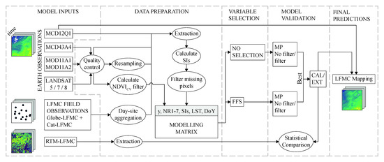
Figure 1.
Overview of the pre-processing, modelling, and analysis steps.
2.2.1. Data Preparation
First, we cropped the Globe-LFMC dataset to the Mediterranean region (Figure 2) and used it, along with the Cat-LFMC, only for the dates with available MODIS data. Then, LFMC samples collected within the same day and site, but corresponding to different species or vegetation layers (e.g., understory and canopy), were aggregated by arithmetic means to obtain a single value per site. Nolan et al. [6] observed that average LFMC per site has a stronger correlation with spectral data than any individual vegetation layer alone. However, some studies have observed that spectral information may more closely reflect signals from the upper part of the canopy, particularly for closed forests [24]. We were interested in developing an indicator of LFMC representative of the entire canopy (upper canopy but also of the understory) because the understory often burns during a fire, which explains why we used the average LFMC value.
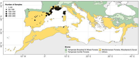
Figure 2.
Distribution of sampling sites and extension of the mapping area for the database and future map productions. The background layer represents terrestrial biomes based on [44]. Gray areas were discarded from map production.
For each resultant LFMC sample, pixel values from remote sensing data were obtained by a simple pixel extraction (that is, the nearest grid cell centroid) matching their sampling date. We performed some preliminary tests observing that the simple pixel extraction method showed no significant differences (p-value = 0.9; see Section S2, Table S1) relative to conducting a focal mean (e.g., from a 3 × 3 window). Afterwards, various vegetation spectral indices (SI; Table S2) potentially related to LFMC were calculated by combining information from different MODIS spectral bands and used as predictors of LFMC in addition to atmospherically corrected reflectance. SI tend to reduce directional anisotropic and soil background effects and highlight specific properties of the vegetation canopy [24]. We also used land surface temperature (LST) from the LST 8-day average composite, as previously discussed (see Section S1). Finally, we added the day of year (DOY) of the ground LFMC samples as auxiliary variables to take into account the seasonal trends in LFMC [22,27]. To do so, DOY was normalized to [0, 1] and reconverted to [−π, π], such that DOY 1 and DOY 366 corresponded to −π and π, respectively. With the resulting values, we calculated the sine (DOY_SIN) and cosine (DOY_COS) to maintain the information on the periodicity as performed in Zhu et al. [34]. Consequently, DOY_SIN varied from −1 to 1 between the wettest and driest season, while DOY_COS varied from winter (coldest; −1) and summer (hottest; 1).
After defining the potential predictors described above (Table 1), we removed LFMC samples with missing data from any variable, and we discarded values outside the threshold 20–250%, which is considered the biological range of LFMC [13]. We then averaged multiple observations in the same day and MODIS-grid cell and randomly assigned the values to one of their locations to have a single daily LFMC value for a given pixel value. The resulting dataset contained a total of 10,374 LFMC field measurements between 2000 and 2019 from 118 sites located in Spain, France, Italy, and Tunisia (Figure 2, Figures S1 and S2). These sites are mostly concentrated in the ecoregions ‘Northeast Spain and Southern France Mediterranean forests’ and ‘Italian sclerophyllous and semi-deciduous forests’ (~80%). Ecoregions with Mediterranean woodlands and coniferous, broadleaf, and mixed forest formations are also represented to a minor degree. In conjunction, mean annual temperature ranges from 6 to 20 °C and mean annual rainfall ranges from 250 to 1100 mm [44]. Site altitude ranges from 11 to 1660 m.
For model validation, Quan et al. [38] RTM data were only acquired for the sample records that coincided with the available dates of such products. We also assigned land cover information from the MCD12Q1 layers to each ground sample by matching the year of sampling with the year of the layer. Misclassified sites (e.g., croplands, permanent wetlands, and urban covers) were discarded or manually corrected based on the species collected, location, and the land cover type field included in the Globe-LFMC database. To simplify the analyses, the IGBP land cover classes present in the study were re-classified into four vegetation (or fuel) types accounting for different structural characteristics (Table S3). These new land cover classes were defined as grasslands, shrublands (closed and open shrublands), savannas (tree cover 10–60%; savannas and woody savannas), and forests (tree cover > 60%; evergreen broadleaf, evergreen needleleaf, and mixed forests).
Additionally, the NDVI coefficient of variation (NDVICV) derived from Landsat data were used to assess the homogeneity of vegetation ‘greenness’ surrounding each site coordinates, as performed in Quan et al. [38]. The authors suggest using these metrics to filter highly heterogeneous areas within a specific satellite footprint since they may not be suitable for predictive attributions [39]. Lower values correspond to more homogeneous sites. NDVICV was calculated with the Landsat surface reflectance values from a 500 × 500 m2 buffer that matched the MODIS cell where site coordinates were located. To do so, we adapted the GEE script publicly shared by Yebra et al. [39], such that the NDVICV value was the monthly average that corresponded to the sampling date. Monthly average maximizes the quality (unmasked pixels) and the stability of the NDVICV statistic. Only values with more than 80% good quality pixels (without no snow, clouds, or shadows) were retained.
2.2.2. Machine Learning Approach
Random forests (RF) was the ML algorithm chosen to empirically estimate LFMC at the Mediterranean basin because of its simplicity, its ability to deal with a large number of covariates, and because it is not necessary to have prior knowledge of the functional form of the relationships between these covariates and the response. Furthermore, the presence of outliers does not have a great influence on its performance [35].
RF is a non-parametric data-driven statistical method proposed by Breiman [45], which is based on Classification and Regression Trees (CART, also called decision trees) and bagging. Several decision trees are constructed in different bootstrap samples of the data, on which every data split (node) is forced to consider an arbitrary subset of available predictors. All individual-tree responses are then aggregated to obtain the final output predictions. The hyperparameters needed for model calibration and used in the subsequent analyses are explained in the associated Supplementary Materials (Table S4). Full details on CART, bagging, and RF can be found in Kuhn and Johnson [35].
2.2.3. Variable Selection: Forward Feature Selection
Variable selection was needed because many of the variables (or features) used as candidates to estimate LFMC were highly correlated with each other, as expected (Figure S3). This is because the SI were formed by close combinations of different spectral bands. On the other hand, predictor variables that are highly autocorrelated in space can be misinterpreted by the RF algorithm, leading to poor predictions outside the locations of the training data [46].
Here, we used the Forward Feature Selection (FFS) method proposed by Meyer et al. [46] to eliminate uninformative predictors and reduce the spatial over-fitting. First, the algorithm trains models using all possible combinations of two predictor variables and keeps those with the lowest prediction error based on a spatial cross-validation that discards entire sampling sites, as described later. Then, FFS iteratively increases the number of variables and evaluates the new model until none of the remaining variables improves the performance of the current best model. Additionally, we introduced a modification of the original method that consisted of calculating the average error over 25 different data splits. This avoided the dependence of cross-validation data splitting and aimed at stabilizing the error estimation [47].
FFS is complex and computationally intensive to execute parallel with RF parameter selection [47], and this step was performed before model calibration using a fixed set of hyperparameters (Table S4).
2.2.4. Model Selection and Performance Evaluation
In order to select the final model, we first assessed the general performance of different forms of the RF (depending on the selected predictors and whether or not the NDVICV filter for heterogeneous pixels was applied) independently from a specific model calibration. We then adjusted the best performing model and evaluated its predictions.
Initial model performance assessment (MP) consisted of a bias-reduced predictive performance evaluation done using a nested 5-fold leave-location-out cross-validation (LLOCV) [47]. Nested cross-validation divides the data two times, first to develop the model and then for independently testing its performance. LLOCV means that the cross-validation folds are made of the observations left out of complete locations, assuring spatial independence [46]. More specifically, the data were divided into 5 outer folds, where one was kept for testing and the remaining were split again into 5 nested folds to iteratively train and select the optimal tuning using a standard LLOCV. Five optimal models were obtained for each outer partition, and the accuracy metrics (described in the section below) were then calculated based on the collection of predictions from all the outer folds. The same procedure was repeated 100 times with different data splits (that is, 500 independent validations), and the overall predictive power metrics were the mean of all repetitions.
Using this method, we assessed MP over 5 different model combinations with the entire set of variables, with the variables selected during the FFS, and with/without applying the NDVICV filter. NDVICV was treated as an additional hyperparameter and implemented in both the whole dataset (training and test) and only to the training partition. The five models consisted of: (1) all variables without filters; (2) all variables with NDVICV filters on the whole dataset; (3) FFS-selected variables without filters; (4) FFS-selected variables with NDVICV filters on the whole dataset; and (5) the best of all/selected variables with the NDVICV filter only applied to the training partition. This method of evaluation provides an appropriate estimate of model reliability since the reported metrics are not a function of a specific model calibration, and many alternative independent datasets (outer folds) are used for testing [47]. Thus, models 1–4 allowed us to examine the effectiveness of the NDVICV filter on the model performance, and the predictive improvement achieved by using only the selected features along with different parameter combinations than the fixed ones in the FFS process. With model 5 we tested how well a model optimized for homogeneous sites (defined by the selected NDVICV value threshold) predicted independent sites that represent both homogeneous and heterogeneous pixels. The best alternative was employed in the subsequent calibration and validation strategies.
After selecting the best approach, we evaluated the predictions by first calibrating the model with LFMC samples from 2000 to 2014 (~80% of the total dataset) and then validated it using the samples collected in 2015–2019 (~20% of the total dataset). That is, we first determined the optimal hyperparameter values for a single model using the samples collected during 2000–2014 by training the algorithm iteratively on one-fifth of the sampling sites and tested on the remaining ones using a standard LLOCV. This process was repeated over 25 random site-resamples for each of the model candidates to stabilize the error rate and eliminate the effect of a particular data partition [47]. The model with the lowest average predictive error was selected and calibrated again to obtain predictions on the whole 5 cross-validation folds. The respective accuracy metrics (called CAL) referred to estimates within the sample period but are not independent from model calibration, as they are the outer-fold metrics in MP. We then evaluated how well the model extrapolates outside the sample period using the samples collected in 2015–2019. This validation phase (named EXT) included some new locations (3 sites) not used in CAL, which means validating future predictions also at unknown points in space.
The final model was used to compare the RF predictions against the RTM estimations produced by Quan et al. [38]. To be a fair comparison, both estimates were contrasted over the same ground-truth samples separately for the LFMCRF predictions inside (CAL) and outside (EXT) the training period.
The optimal hyperparameters for model calibration were chosen from an initial set of possible inputs performing a grid-search scheme [47]. We considered a wider range of possible values (Table S4) of the grid-search scheme for the MP, and then we limited the range according to the results obtained from all fitted models. For CAL, each parameter combination in the grid was iteratively assessed. In the MP, a random subset of combinations (e.g., 50) was implemented at each training process to be more computationally effective. In this case, the choice of hyperparameters was not so important since the cross-validation estimates were a generalization of the model performance.
In all cases, models were optimized to predict new locations, which is the interest of remote sensing(that is, to estimate LFMC over areas without available ground data), and it prevents spatial over-fitting [46]. For MP and CAL grid-search steps, these locations were selected using the method of Meyer et al. [46] to benefit splitting diversity. In the final model adjustment, prior to predictions, sample-site splitting was conducted by means of their coordinates and the K-means algorithm to ensure equal spatial distribution [48].
2.2.5. Validation Methods and Map Production
The predictive capabilities of the model were characterized by means of the root mean square error (RMSE), the mean absolute error (MAE), the mean bias error (MBE), and the unbiased RMSE (ubRMSE), as well as the variance explained by predictive models based on cross-validation (VEcv) [49] and the Lin’s concordance correlation coefficient (CCC) [50]. RMSE, MAE, and MBE measure, respectively, squared, absolute, and mean departures between the estimated and observed test values of LFMC in the same units of the outcomes. RMSE was the statistic used as a criterion for parameter tuning and variable selection processes. We included the ubRMSE following Zhu et al. [34], which shows the error after removing the tendency to over- or under-predict in the model:
Here, n is the number of observations in a validation dataset. VECV is similar to the coefficient of determination R2, but it measures the predictive accuracy of a model by comparing observations and predictions derived from cross-validation and not the square correlation between observed and fitted values. It is defined as:
where is the mean of the observed values. Otherwise, CCC provides a measure of correlation relative to the line of agreement, which is expected to be unbiased with a slope of 1 and apply a penalty (Cb) if the relationship is far from this line. From CAL, EXT, and the RTM, we also obtained the slope and intercept from the linear regression between observed against predicted to assess general deviation trends.
Spatiotemporal analyses were additionally made through land cover types [31]. More specifically, we calculated general performance metrics from the CAL and EXT estimates for each land cover class, and we decomposed the mean RMSE by land cover and the month of the year to determine the temporal variability of the predictions over each vegetation functional type.
After the validations, we recalibrated the model using the whole dataset in order to consider all the available information to train the algorithm. The readjusted LFMCRF was then used to produce the collection of maps of the reported LFMC database.
2.2.6. Marginal Effects of the Predictors
We used partial dependence plots derived from the fitted model to evaluate the contribution of each variable to the LFMC estimations. The partial dependence function represents the average effect of a given variable on the predicted response marginalized over the effects of the rest of model inputs [51]. Mainly, we divided the distribution of values of the variable of interest into equal steps (e.g., 50). At each step, we calculated the average of all possible predictions made on the data holding the value of the step constant. Finally, we drew a line joining all average points. Resulting plots allowed for the examination of the functional relationships between the most relevant features and the LFMC estimates.
2.2.7. Software
Model building and statistical analysis were made with the statistical software R version 4.2.0 [52] and their base package for generic operations. RF was principally implemented with the R package ‘ranger’ [53] but also with the ‘randomForest’ library [54] to extract the partial dependence plots. The R packages ‘raster’ [55] and ‘sf’ [56] were used for remote sensing and spatial data manipulation, and ‘doParallel’ [57] for parallel computing. An adaptation of the stratfold3d function of the ‘sparsereg3D’ package [48] was used to make the equally spatially distributed LLOCV folds, while the spatially random splits were created with the CreateSpacetimeFolds function from the ‘CAST’ package [58].
3. Results
3.1. Selected Variables
Results of the FFS indicated that the most important predictors of LFMC, in terms of error reduction, were the combination of LST and DOY_SIN followed by VARI, NDTI, and DOY_COS (Figure 3). These five variables alone led to an RMSE of 20.1%. We also considered NR3 and NR5 because each one represented on average an additional improvement of ~0.1% in RMSE from the previous stepwise selection, which was greater than the corresponding RMSE standard error (~0.05%) calculated from the 25 FFS realizations. Selected variables for the subsequent developments reached an overall RMSE of 19.9%.
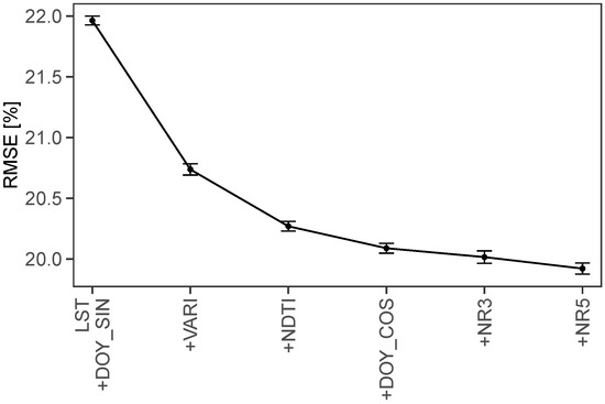
Figure 3.
Selected variables derived from the combination of the Forward Feature Selection (FFS) process and the leave-location-out cross-validation (LLOCV). Black dots and vertical segments represent, respectively, the average LLOCV error and the standard error calculated from the 25 random forests computed at each FFS step.
3.2. Statistical Performance of the LFMCRF
Calibrated and evaluated models within the general model performance assessment (MP) achieved similar results among them, with overall RMSEs (that is, from all separate iterations of each MP alternative in conjunction) ranging from 19.1% to 21.4% and VECV ranging from 0.28 to 0.43. Average performance statistics (Table 2) showed that all MP alternatives tended towards a slight overprediction (MBE: 0.9–1.5%). Nonetheless, the ubRMSE values were close to the RMSE (max. difference ~0.07%), further indicating a relatively low bias of the LFMCRF estimates. In general, models with all the initial predictors (Allp) showed worse performance than those with only the selected ones (Selp) (Table 2). The latter benefited from the elimination of the spatially dependent variables and were used in the successive validation strategies.
Table 2.
Evaluation metrics from predicted and observed values of the model performance (MP), spatial cross-validation (CAL), and the time extrapolation (EXT) assessment. Different methods based on the NDVICV filter application and the complete (Allp) or selected (Selp) predictive variables. Predictions from CAL and EXT broken down by fuel type. RTM extractions and LFMCRF were validated on the same ground-truth observations separately if they were used in CAL or EXT.
Application of the NDVICV filter did not show significant effects on the general model performance (Table 2; Figures S4 and S5). For example, applying the optimal filter in Selp to the entire dataset (F1) led to a small improvement in RMSE (<2%) and VECV (~0.01), but also to an increase of MBE (~0.15%) with respect to no filter application. Moreover, comparing MP with no filter and with the filter only applied to the training data (F2) resulted in increases in RMSE and MBE by 0.02% and 0.2%, respectively. In addition, the application of the filter led to the elimination of 26–28% of the dataset. It is worth noting that only a very small percentage of the data (2–4%) was deleted with NDVICV application because they were above the optimal filter threshold (0.3–0.35). The rest of the data was removed because of missing rows in NDVICV, which were derived from poor-quality pixels in Landsat products. The model with no filter was thus used in subsequent analyses.
3.3. Prediction Assessment and Intercomparison
Accuracy metrics from the calibrated model (CAL) were consistent with the general performance (MP) of the LFMCRF (Table 2). These results were expected because CAL was developed with 80% of the data employed in MP, but they proved that the adjusted model was not overfitted to the particular data or by the current hyperparameter optimization (Table S4). In contrast, the EXT validation showed smaller RMSE (~3.5%) and higher VECV (~0.15) than CAL, probably due to differences in the validation samples.
We did not observe any significant bias in the LFMCRF estimations, as the y-intercepts and slopes were close to 0 and 1 in the fitted line between measured and predicted values of LFMC, respectively (Figure 4a,d). However, the residuals between predictions and observations revealed a linear pattern along the range of LFMC in both CAL and EXT (Figure S6). For example, the model highly underestimated values above 120% (MBE CAL = −33.97% and MBE EXT = −22.58%) and overestimated values below 30% (MBE CAL = 45.7%; no data in EXT). This explained the aforementioned better outcomes from EXT, because the range of the actual LFMC for testing (31–209%) excluded values where the model performed worst. Within the LFMC values (30–120%) where live fuels transition from flammable to non-flammable, the model attained a smaller RMSE (MAE) of 16.75% (13.35%) for CAL and 15.10% (12.19%) for EXT relative to the overall performance of the corresponding estimates, with a small propensity to overestimate (MBE of 3.30% and 5.24% for CAL and EXT, respectively). It is worth noting that 92% of the data was within the range of 30–120%, and data below 30% may have represented curing.
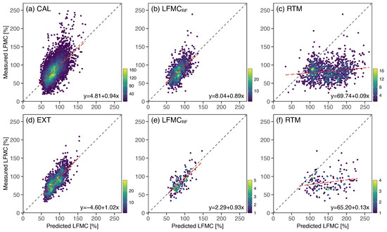
Figure 4.
LFMC field measurements versus predictions from CAL (upper plots) and EXT (lower plots): all predictions (a,d), LFMCRF predictions made on the same data points available in RTM (b,e), and the corresponding RTM (c,f). Dashed black line and red line indicates the expected 1:1 relationship and the fitted linear model, respectively. Color scale indicates point density.
LFMCRF had better performance than RTM-based estimates when comparing against the same validation samples. In fact, poor correlation and large errors between observed and predicted values occurred in RTM simulations (Table 2). RTM systematically overpredicted LFMC when LFMC exceeded ~76% (Figure 4c,f). Negative values of VECV (−10.15 and −8.98) indicated that these LFMC estimates were less accurate than using the mean of observations as predictions. Otherwise, the LFMCRF estimations used for this comparison showed the same level of accuracy as in the previous sections (Figure 4b,e), given that they were subsets of predictions from CAL and EXT.
3.4. Evaluation across Vegetation Types
Assessing the performance across vegetation types, LFMCRF reached better results in EXT (RMSE: 12–17%; CCC: 0.6–0.7) than in CAL (RMSE: 18–23%; CCC: 0.5–0.6) for all fuel types (Table 2). This coincides with previous results and may be because of the greater range in LFMC variation observed in the CAL dataset (Figure S2). Forests showed the smallest errors in CAL (MBE = 0.87%; RMSE = 18.32%), but the largest in EXT (MBE = 7.40%; RMSE = 16.87%). Grasslands obtained the best performance within the EXT validation (Table 2). However, they represented < 3% of the validation records and were mainly concentrated (~80% of the total) in Jul–Aug, where the model performed better (Figure 5c,d). In both cases, LFMCRF significantly underpredicted LFMC in shrublands (MBE −7.76 to −4.62). Temporally, the smallest errors (RMSE: 16–19%) were obtained during the hottest months (Jul–Aug), where field samples were primarily collected (Figure 5a,b), and also in winter months (Jan–Feb), matching with the lowest LFMC variability (Figure S2d). Forests showed larger stability during the entire year in both RMSE (Figure 5c) and LFMC measurements (Figure S2c). Contrarily, the performance of the model greatly fluctuated in grasslands. Grasslands reported the largest RMSE (36.7%) in May, one of the wettest months of the Mediterranean region, when fires are scarce, declining to an RMSE of 14.9% (Figure 5c) during the driest month.
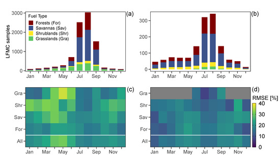
Figure 5.
Number of testing samples and RMSE from CAL (a,c) and EXT (b,d) by vegetation type and month of the year. Gray cells in c and d indicate no data available. The IGBP classes from MCD12Q1 were aggregated by the vegetation functional type to which they belong.
3.5. Marginal Effects of the Predictors
Partial dependence plots exposed different patterns on the variation of LFMC estimates (Figure 6). VARI and DOY_SIN exerted the strongest effects on predictions. LFMCRF estimates monotonically increased as the VARI values increased. Conversely, LFMC generally monotonically decreased with increases of DOY_SIN, indicating that the highest LFMC values occurred in spring (−1) and the lowest in late summer (1). LST had non-significant effects on the LFMC estimations up to 20 °C but then presented a clear negative relationship. NR5 showed a concave shape, with marked increases at higher values of NR5 (>0.3; last decile). NDTI, NR3, and DOY_COS showed little effects on the predictions of LFMC, but they were still considered informative. The partial dependence of DOY_COS on the LFMC prediction may have been masked by the marginal effects of LST, as they were highly correlated (Figure S3).
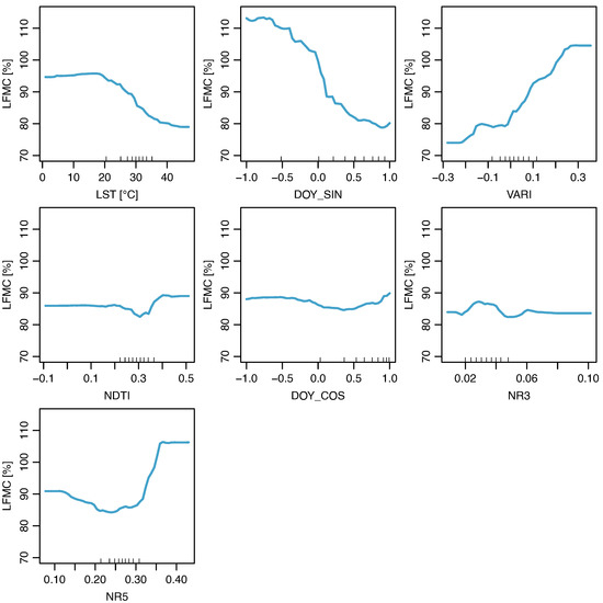
Figure 6.
Partial dependence plots from the fitted model. Blue lines describe the average effect of a given predictor in the LFMC estimates. Small lines in the x axis indicate the deciles of the predictor values.
4. Discussion
We propose a novel method to estimate LFMC from remote sensing at the subcontinental scale by means of a selected set of remote sensing predictors and the RF algorithm. LFMCRF outperforms current approaches used in the Western Mediterranean basin in terms of validation errors and provides a solid alternative to predict LFMC over a wide range of environmental conditions using a simple but robust model with a unique formulation. In the next sections, we discuss the contribution of each selected predictor, the general and the spatiotemporal performance of the model, as well as their potential applicability and future improvements.
4.1. Selected Predictors
The key explanatory features derived from the FFS process were the variables derived from the day of the year (DOY_COS, DOY_SIN), LST, VARI, and NDTI, along with nadir reflectance bands 3 (blue) and 5 (NIR) to a minor degree.
DOY_SIN and DOY_COS had a significant influence on the LFMC estimates due to the seasonal variation in LFMC. In general, LFMC dynamics follow the distribution of the balance between evapotranspiration and rainfall in the Mediterranean region [21,26,34]. DOY_SIN partly reflects the average annual pattern in soil water availability and acts as a complement of the SI, maintaining the periodicity of LFMC within the year. Similarly, DOY_COS reflects changes in the temperature and is more related to vegetation surface temperature, which is measured by the LST [22,27].
As we expected, LST was a key factor explaining LFMC, and it showed a negative relationship with LFMC when temperatures were above ~20 °C [22,27,28]. LST is a key determinant of the energy balance of the vegetation, and its difference with air temperature is related to evapotranspiration and water losses [59]. Such differences between air temperature and LST depend on the density of vegetation cover, and previous works have shown strong relationships when combining LST and a vegetation index (e.g., [27]), as was done here. DOY_COS and LST are complementary because the former keeps the inter-annual variation of LFMC trends, while the latter provides better spatial information (that is, local deviations from the average trends) [27]. The partial dependence of LFMC on LST was similar to that reported in previous studies in that LST only affected LFMC after a certain temperature threshold [28]. LST is related to VPD [60], which is a variable that can also affect plant water content as a primary driver of evapotranspiration [61]. The importance of LST may thus be related to the fact that VPD significantly acts on leaf moisture content after a certain threshold is reached. Therefore, it is also possible that LST could be reflecting local differences in surface temperature and VPD. Further work is needed to fully understand the mechanisms by which LST affects LFMC.
VARI combines different visible wavelength bands (blue–green–red), and it has the ability to detect chlorophyll content and leaf structure variations, which are indirectly associated with changes in canopy moisture [19]. Several authors [15,19,23,26,30] have shown that VARI is one of the best indices for predicting LFMC on different vegetation types, and we also demonstrated a notable dependency of the LFMCRF estimations (Figure 6). Other authors found stronger correlations with indices that include SWIR [37] and NIR [21,62] bands predicting LFMC at local scales.
Reductions in chlorophyll content can result from water shortage but also from changes in leaf age, nutrient deficiency, health, and phenological stages [33,63]. Introducing NDTI from SWIR bands in the spectral region greatly sensitive to plant water content [33,64], was necessary to correct for VARI changes not driven by the moisture status of plants. Moreover, Wang et al. [63] described a connection (r = 0.45) between NDTI and dry matter content of vegetation. Dry matter weight is the denominator of the LFMC equation and could lead to variations in the spectral response and LFMC due to plant seasonal growth, independently of drought changes [30,65].
On the other hand, NIR (NR5, centered at 1240 nm) is partly influenced by water content but also by leaf internal structure and dry biomass [33,65]. This particularity may explain the concave effect that this variable had on predictions. Water loss produces an increment of NR5 as a result of lower water absorption [64]. However, at certain species and LFMC levels, water stress leads to leaf cell structure changes (reducing reflective areas by wilting) and leaf curling, which cause a decrease in NR5 [24,64].
We acknowledge that topography could have affected our results as it alters microclimatic variables influencing LFMC, such as solar radiation. However, a previous study that used reflectance bands as main explanatory variables [34] indicated a rather small effect on LFMC estimations with an RMSE improvement of ~1%.
4.2. Model Performance Assessment
Generalization errors of the LFMCRF (RMSE: 16–20%; MAE: 13–15%) were lower than in other studies attempting to model LFMC at large spatial scales. For instance, Zhu et al. [34] reported an overall RMSE of 27.9% using a similar spatial validation strategy but for the contiguous US. They also achieved an RMSE of 22.7% performing a standard cross-validation, which normally results in higher accuracy because the training and testing sets are not spatially independent. LFMCRF also showed smaller RMSE than did Rao et al. [31] (25%), who used the same spatial approach as Zhu et al. [34] but ignored multi-species sites with high LFMC seasonal variation, where predictions tend to be more uncertain.
The proposed model tended to underestimate large values and overestimate small values of LFMC (Figure S6). Poor performance of an RF-based model towards the extremes is a well-known problem within RF models [35]. Nonetheless, similar problems were also reported in previous works based on machine learning [34,36], classical regression [23,26] and RTM simulation [20] methods. One reason for the systematic bias at high moisture levels can be the lower sensitivity of optical spectra to capture changes in water content while the vegetation gets wet [25,38]. Our strategy to address this problem was to assess LFMC over a very wide range, such that extreme values, those where LFMC estimation is problematic, are largely out of range. The lower level of LFMC in this study was 20%, but fuel moisture below 30% often corresponds to dead fuel (e.g., cured grass) and is thus beyond our scope, since we were interested in LFMC [24]. Similarly, the higher LFMC values (above 200%) may be related to harvested samples with the presence of primary tissues from a new vegetative period [21], plant parts other than leaves (e.g., fruits, flowers), or the inadequately inclusion of samples collected after rain or dew events [20].
The LFMCRF showed a better performance that RTM predictions from Quan et al. [38]. The RTM-based estimates were highly biased with a strong tendency to overpredict beyond 76% LFMC. This coincided with the results reported by Marino et al. [26], who found an identical pattern starting at the threshold of 65% using the RTM developed by Yebra et al. [20]. This demonstrates a better predictive power for our data-driven approach, even though physically-based approaches are expected to be more precise when applied to sites not used for calibration [24]. At any rate, we acknowledge that comparing a regional dataset like this one against a global dataset is not entirely fair, given the scale gap, but our results highlight that the RMSE of the global RTM hinders any local application for operational purposes.
The critical LFMC level associated with fire occurrence in the Mediterranean forests, and other parts of the world occurs around 100% [5,6,7]. Our model improves current products, but MAE around the critical threshold of 100% LFMC is still ~13%. Differences of 10% in LFMC estimation from field measurements are generally acceptable for fire management [26]. However, these results indicate that there is still room for further improvements, particularly towards the critical threshold, so as to avoid reporting of false fire alerts or omission of danger situations [19].
4.3. Evaluation across Vegetation Types
The predictive errors obtained by the LFMCRF within the training period for forests/savannas (RMSE 18–20%), shrublands (RMSE ~21%), and grasslands (RMSE ~23%) were similar between them and comparable to those reported by other studies for the same vegetation types (forests/savannas 22–32%, shrublands 14–29%, grasslands 29–49%) [18,20,31,34,38]. Despite the methodological differences, this comparison demonstrates that a single model can be as accurate or even better than formalizing a model for each fuel class separately. This could be due to the RF architecture that allows using the spectral and thermal information itself to discriminate between vegetation functional types. Furthermore, misclassification problems of the land cover products used to differentiate between fuel classes can further increase the uncertainty of the LFMC estimates [20,34].
In general, we observed that the uncertainty of the LFMC predictions (Figure 5) depended on the range of LFMC values for testing and their local and temporal variability (Figure S2). For example, forests showed more stable behavior in both LFMC dynamics and prediction agreement. Deep root systems in trees reduce the seasonal LFMC variation [2]. On the contrary, grasslands reported the highest errors in spring (the wettest part of the year) and the lowest in the driest periods (summer, when fires are more likely). These patterns overlapped with the monthly maximum and minimum values of LFMC, that is, larger LFMC errors under higher LFMC values and smaller LFMC errors under lower values. Shrublands instead had a low temporal variability but presented a significant bias (MBE from −5 to −8%), likely because of the high proportion of large LFMC values (>120%) in their ground-truth sample distributions (16.4% of the total ground-truth samples). The error associated with predictions outside the training period (EXT) was similar to that from the CAL dataset (Figure 5). However, RMSE was slightly lower with the EXT dataset because of the lower LFMC variability in the EXT dataset relative to CAL. We thus conclude that the fitted model with historical data can be safely applied in future situations without the need for frequent readjustment, but with careful interpretation in the wettest months and for LFMC values below 30%.
4.4. Applicability and Potential Improvements
The relatively coarse resolution (~500 m) of the final product is appropriate for landscape-scale use and does not guarantee smaller-scale applications. Each individual pixel normally contains information from a mixture of vegetation canopy layers, species, surface litter, and soil elements with different properties that cannot be unambiguously separated [10,20]. We acknowledge that a limitation to this study is that we did not explicitly assess the representativeness of the samples within the site. We therefore took into account small-scale heterogeneity by implementing an NDVICV filter, as in Quan et al. [38]. However, we did not observe any significant improvement after applying this filter, likely indicating that sample areas were relatively homogenous. In any case, sub-pixel variation and the scale mismatch between sample-plot size and pixel resolution hinder establishing relationships between field observations and satellite-derived variables, introducing uncertainties into the predictions. The latter could be solved using higher spatial resolution data (e.g., Sentinel-2 or Landsat) [26,36,37,62], but these satellites usually have lower revisit frequency disabling near-real-time usage and introducing a time lag between the images and the sampling date [26]. Future work should extend the use of our methods to these newer satellites because historical LFMC field data currently available is not yet sufficient to achieve this goal.
Further progress will come from joining our approach with microwave remote sensing data. Microwave observations (active and passive) can also detect changes in vegetation water content but are less sensitive to atmospheric conditions (e.g., clouds) than optical wavelengths [30] and have the ability to penetrate deeper into the canopies [31]. The recently available non-commercial radar data supplied by the Sentinel-1 A/B Synthetic Aperture Radar (SAR) may represent a great opportunity to infer the improvement of LFMC models at the operational level [31,32].
Sample representativeness is a general constrain in the empirical models [24]. In this study, field samples were not evenly distributed across the whole Mediterranean basin. They could be considered representative of the Western Mediterranean conditions since they were abundant in number (space and time) within their specific biome, as well as in species and environmental conditions. Thus, application of the LFMCRF should be limited to areas with similar characteristics, and LFMC estimates must be interpreted with caution in underrepresented areas (e.g., temperate zones). Despite that, the generated maps extend to the entire Mediterranean biome included in the Mediterranean basin, as well as some meridional areas of the temperate biomes of Europe (e.g., northern Spain) (Figure 2).
5. Conclusions
We successfully tested an RF algorithm as an approach to predict large-scale LFMC using the spectral and thermal information of MODIS and two static variables representing seasonal patterns. The LFMCRF is applicable to a wide variety of vegetation types, and the performance of the fitted model (MBE = 0.47%, RMSE = 19.9%, VECV = 0.37, CCC = 0.56) was comparable to that of other studies with similar purposes but with a higher degree of complexity than LFMCRF, including the RTM-based methods with applications in the Mediterranean basin. The architecture of RF allows the introduction of new explanatory variables that would help to reduce the uncertainty in the predictions. LFMC maps were produced at 8-day intervals from 2001 to 2021. The final product provides a complete asset for studying the relationships between LFMC and the influencing factors that promote wildfire activity and fire regimes in the Mediterranean basin. Furthermore, after the imminent MODIS decommission, the new Visible Infrared Imaging Radiometer Suite (VIIRS) is expected to provide long-term continuity with better spatial resolution [24]. Continuous retrievals, either with MODIS or VIIRS, might be a valuable tool for quasi near-real-time fire risk assessment and for operational applications such as the mobilization of resources and people or the planning of preventive actions for fire mitigation (e.g., fuel reduction or prescribed burns).
Supplementary Materials
The following supporting information can be downloaded at: https://www.mdpi.com/article/10.3390/rs14133162/s1, Table S1. Performance metrics from the focal mean and simple pixel extraction comparison; Table S2. Spectral vegetation indices used to estimate LFMC; Table S3. Land cover classes from samples used in the study; Table S4. Boundaries of the RF hyperparameters grid-search space, adjusted parameters for the Forward Feature Selection (FFS) process and optimized hyperparameters for the final model; Figure S1. LFMC ground samples overall and by country distributions; Figure S2. Mean and standard deviation (SD) matrices from CAL and EXT of the LFMC field measurements shown by fuel type and month of the year, and the overall of each one; Figure S3. Correlation matrix between LFMC and predictive variables; Figure S4. Performance metrics profiles from the general model performance assessment (MP) alternative with the selected variables and the NDVICV filter applied to the entire dataset and only to the training partition; Figure S5. LFMC field observations versus predictions from the CAL validation theoretically rejected by the 0.3 NDVICV threshold; Figure S6. Residuals between predictions and observations against the LFMC observations and their marginal density distributions for CAL and EXT. This SM are distributed in 8 sections of additional methods and analyses: S1, Land surface temperature; S2, Data extraction method [66]; S3, Spectral vegetation indices; S4, Land cover definitions; S5, Model parametrization [67]; S6, Data description; S7, NDVICV filter; S8, Additional prediction analysis.
Author Contributions
Conceptualization, À.C.C., P.G.-M. and V.R.d.D.; investigation, À.C.C.; formal analysis, À.C.C.; writing—original draft preparation, À.C.C.; writing—review and editing, P.G.-M. and V.R.d.D. All authors have read and agreed to the published version of the manuscript.
Funding
This study was funded by the MICINN (RTI2018-094691-B-C31), European Union’s Horizon 2020-Research and Innovation Framework Programme under grant agreement no. 101003890 project FirEUrisk, the National Natural Science Foundation of China (U20A20179, 31850410483), and the talent proposals in Sichuan Province (2020JDRC0065) from Southwest University of Science and Technology (18ZX7131).
Data Availability Statement
All the scripts and data generated and analyzed during the current study are publicly available in the Github repository, https://github.com/fuegologos/lfmc_rf. The final product of the weekly LFMC maps is fully available at 10.5281/zenodo.6784663.
Acknowledgments
We remain indebted to Xingwen Quan for providing us the RTM-based LFMC data.
Conflicts of Interest
The authors declare no of interest.
References
- Bradstock, R.A. A Biogeographic Model of Fire Regimes in Australia: Current and Future Implications. Glob. Ecol. Biogeogr. 2010, 19, 145–158. [Google Scholar] [CrossRef]
- Resco de Dios, V. Plant-Fire Interactions: Applying Ecophysiology to Wildfire Management, Managing Forest Ecosystems; Managing Forest Ecosystems; Springer International Publishing: Cham, Switzerland, 2020; Volume 36, ISBN 978-3-030-41191-6. [Google Scholar]
- Jolly, W.; Johnson, D. Pyro-Ecophysiology: Shifting the Paradigm of Live Wildland Fuel Research. Fire 2018, 1, 8. [Google Scholar] [CrossRef] [Green Version]
- Nelson, R.M. Water Relations of Forest Fuels. In Forest Fires: Behavior and Ecological Effects; Johnson, E.A., Miyanishi, K., Eds.; Academic Press: San Diego, CA, USA, 2001; pp. 79–149. [Google Scholar]
- Dennison, P.E.; Moritz, M.A. Critical Live Fuel Moisture in Chaparral Ecosystems: A Threshold for Fire Activity and Its Relationship to Antecedent Precipitation. Int. J. Wildland Fire 2009, 18, 1021. [Google Scholar] [CrossRef]
- Nolan, R.H.; Boer, M.M.; de Dios, V.R.; Caccamo, G.; Bradstock, R.A. Large-Scale, Dynamic Transformations in Fuel Moisture Drive Wildfire Activity across Southeastern Australia. Geophys. Res. Lett. 2016, 43, 4229–4238. [Google Scholar] [CrossRef] [Green Version]
- Luo, K.; Quan, X.; He, B.; Yebra, M. Effects of Live Fuel Moisture Content on Wildfire Occurrence in Fire-Prone Regions over Southwest China. Forests 2019, 10, 887. [Google Scholar] [CrossRef] [Green Version]
- IPCC. Climate Change 2022: Impacts, Adaptation, and Vulnerability. Contribution of Working Group II to the Sixth Assessment Report of the Intergovernmental Panel on Climate Change; Pörtner, H.-O., Roberts, D.C., Tignor, M., Poloczanska, E.S., Mintenbeck, K., Alegría, A., Craig, M., Langsdorf, S., Löschke, S., Möller, V., et al., Eds.; IPCC: Geneva, Switzerland, 2022. [Google Scholar]
- Dupuy, J.; Fargeon, H.; Martin-StPaul, N.; Pimont, F.; Ruffault, J.; Guijarro, M.; Hernando, C.; Madrigal, J.; Fernandes, P. Climate Change Impact on Future Wildfire Danger and Activity in Southern Europe: A Review. Ann. For. Sci. 2020, 77, 35. [Google Scholar] [CrossRef]
- Chuvieco, E.; Aguado, I.; Salas, J.; García, M.; Yebra, M.; Oliva, P. Satellite Remote Sensing Contributions to Wildland Fire Science and Management. Curr. For. Rep. 2020, 6, 81–96. [Google Scholar] [CrossRef]
- Boer, M.M.; Nolan, R.H.; De Dios, V.R.; Clarke, H.; Price, O.F.; Bradstock, R.A. Changing Weather Extremes Call for Early Warning of Potential for Catastrophic Fire. Earth’s Future 2017, 5, 1196–1202. [Google Scholar] [CrossRef]
- Gabriel, E.; Delgado-Dávila, R.; De Cáceres, M.; Casals, P.; Tudela, A.; Castro, X. Live Fuel Moisture Content Time Series in Catalonia since 1998. Ann. For. Sci. 2021, 78, 44. [Google Scholar] [CrossRef]
- Martin-StPaul, N.; Pimont, F.; Dupuy, J.L.; Rigolot, E.; Ruffault, J.; Fargeon, H.; Cabane, E.; Duché, Y.; Savazzi, R.; Toutchkov, M. Live Fuel Moisture Content (LFMC) Time Series for Multiple Sites and Species in the French Mediterranean Area since 1996. Ann. For. Sci. 2018, 75, 70. [Google Scholar] [CrossRef] [Green Version]
- Van Wagner, C.E. Development and Structure of the Canadian Forest Fire Weather Index System. Canadian Forestry Service. For. Technol. Rep. 1987, 35, 37. [Google Scholar]
- Caccamo, G.; Chisholm, L.A.; Bradstock, R.A.; Puotinen, M.L.; Pippen, B.G. Monitoring Live Fuel Moisture Content of Heathland, Shrubland and Sclerophyll Forest in South-Eastern Australia Using MODIS Data. Int. J. Wildland Fire 2012, 21, 257. [Google Scholar] [CrossRef]
- Ruffault, J.; Martin-StPaul, N.; Pimont, F.; Dupuy, J.-L.L. How Well Do Meteorological Drought Indices Predict Live Fuel Moisture Content (LFMC)? An Assessment for Wildfire Research and Operations in Mediterranean Ecosystems. Agric. For. Meteorol. 2018, 262, 391–401. [Google Scholar] [CrossRef]
- Martin, M.S.; Bonet, J.A.; De Aragón, J.M.; Voltas, J.; Coll, L.; De Dios, V.R. Crown Bulk Density and Fuel Moisture Dynamics in Pinus Pinaster Stands Are Neither Modified by Thinning nor Captured by the Forest Fire Weather Index. Ann. For. Sci. 2017, 74, 51. [Google Scholar] [CrossRef]
- Jurdao, S.; Yebra, M.; Guerschman, J.P.; Chuvieco, E. Regional Estimation of Woodland Moisture Content by Inverting Radiative Transfer Models. Remote Sens. Environ. 2013, 132, 59–70. [Google Scholar] [CrossRef]
- Yebra, M.; Chuvieco, E.; Riaño, D. Estimation of Live Fuel Moisture Content from MODIS Images for Fire Risk Assessment. Agric. For. Meteorol. 2008, 148, 523–536. [Google Scholar] [CrossRef]
- Yebra, M.; Quan, X.; Riaño, D.; Larraondo, P.R.; van Dijk, A.I.J.M.; Cary, G.J. A Fuel Moisture Content and Flammability Monitoring Methodology for Continental Australia Based on Optical Remote Sensing. Remote Sens. Environ. 2018, 212, 260–272. [Google Scholar] [CrossRef]
- Argañaraz, J.P.; Landi, M.A.; Bravo, S.J.; Gavier-Pizarro, G.I.; Scavuzzo, C.M.; Bellis, L.M. Estimation of Live Fuel Moisture Content From MODIS Images for Fire Danger Assessment in Southern Gran Chaco. IEEE J. Sel. Top. Appl. Earth Obs. Remote Sens. 2016, 9, 5339–5349. [Google Scholar] [CrossRef]
- Chuvieco, E.; Cocero, D.; Riaño, D.; Martin, P.; Martínez-Vega, J.; de la Riva, J.; Pérez, F. Combining NDVI and Surface Temperature for the Estimation of Live Fuel Moisture Content in Forest Fire Danger Rating. Remote Sens. Environ. 2004, 92, 322–331. [Google Scholar] [CrossRef]
- Peterson, S.H.; Roberts, D.A.; Dennison, P.E. Mapping Live Fuel Moisture with MODIS Data: A Multiple Regression Approach. Remote Sens. Environ. 2008, 112, 4272–4284. [Google Scholar] [CrossRef]
- Yebra, M.; Dennison, P.E.; Chuvieco, E.; Riaño, D.; Zylstra, P.; Hunt, E.R.; Danson, F.M.; Qi, Y.; Jurdao, S. A Global Review of Remote Sensing of Live Fuel Moisture Content for Fire Danger Assessment: Moving towards Operational Products. Remote Sens. Environ. 2013, 136, 455–468. [Google Scholar] [CrossRef]
- Yebra, M.; Chuvieco, E. Linking Ecological Information and Radiative Transfer Models to Estimate Fuel Moisture Content in the Mediterranean Region of Spain: Solving the Ill-Posed Inverse Problem. Remote Sens. Environ. 2009, 113, 2403–2411. [Google Scholar] [CrossRef]
- Marino, E.; Yebra, M.; Guillén-Climent, M.; Algeet, N.; Tomé, J.L.; Madrigal, J.; Guijarro, M.; Hernando, C. Investigating Live Fuel Moisture Content Estimation in Fire-Prone Shrubland from Remote Sensing Using Empirical Modelling and RTM Simulations. Remote Sens. 2020, 12, 2251. [Google Scholar] [CrossRef]
- García, M.; Chuvieco, E.; Nieto, H.; Aguado, I. Combining AVHRR and Meteorological Data for Estimating Live Fuel Moisture Content. Remote Sens. Environ. 2008, 112, 3618–3627. [Google Scholar] [CrossRef]
- McCandless, T.C.; Kosovic, B.; Petzke, W. Enhancing Wildfire Spread Modelling by Building a Gridded Fuel Moisture Content Product with Machine Learning. Mach. Learn. Sci. Technol. 2020, 1, 035010. [Google Scholar] [CrossRef]
- Sow, M.; Mbow, C.; Hély, C.; Fensholt, R.; Sambou, B. Estimation of Herbaceous Fuel Moisture Content Using Vegetation Indices and Land Surface Temperature from MODIS Data. Remote Sens. 2013, 5, 2617–2638. [Google Scholar] [CrossRef] [Green Version]
- Fan, L.; Wigneron, J.-P.; Xiao, Q.; Al-Yaari, A.; Wen, J.; Martin-StPaul, N.; Dupuy, J.-L.; Pimont, F.; Al Bitar, A.; Fernandez-Moran, R.; et al. Evaluation of Microwave Remote Sensing for Monitoring Live Fuel Moisture Content in the Mediterranean Region. Remote Sens. Environ. 2018, 205, 210–223. [Google Scholar] [CrossRef]
- Rao, K.; Williams, A.P.; Flefil, J.F.; Konings, A.G. SAR-Enhanced Mapping of Live Fuel Moisture Content. Remote Sens. Environ. 2020, 245, 111797. [Google Scholar] [CrossRef]
- Wang, L.; Quan, X.; He, B.; Yebra, M.; Xing, M.; Liu, X. Assessment of the Dual Polarimetric Sentinel-1A Data for Forest Fuel Moisture Content Estimation. Remote Sens. 2019, 11, 1568. [Google Scholar] [CrossRef] [Green Version]
- Ceccato, P.; Flasse, S.; Tarantola, S.; Jacquemoud, S.; Grégoire, J.-M. Detecting Vegetation Leaf Water Content Using Reflectance in the Optical Domain. Remote Sens. Environ. 2001, 77, 22–33. [Google Scholar] [CrossRef]
- Zhu, L.; Webb, G.I.; Yebra, M.; Scortechini, G.; Miller, L.; Petitjean, F. Live Fuel Moisture Content Estimation from MODIS: A Deep Learning Approach. ISPRS J. Photogramm. Remote Sens. 2021, 179, 81–91. [Google Scholar] [CrossRef]
- Kuhn, M.; Johnson, K. Applied Predictive Modeling; Springer: New York, NY, USA, 2013; ISBN 978-1-4614-6848-6. [Google Scholar]
- Adab, H.; Kanniah, K.D.; Beringer, J. Estimating and Up-Scaling Fuel Moisture and Leaf Dry Matter Content of a Temperate Humid Forest Using Multi Resolution Remote Sensing Data. Remote Sens. 2016, 8, 961. [Google Scholar] [CrossRef] [Green Version]
- Costa-Saura, J.M.; Balaguer-Beser, Á.; Ruiz, L.A.; Pardo-Pascual, J.E.; Soriano-Sancho, J.L. Empirical Models for Spatio-Temporal Live Fuel Moisture Content Estimation in Mixed Mediterranean Vegetation Areas Using Sentinel-2 Indices and Meteorological Data. Remote Sens. 2021, 13, 3726. [Google Scholar] [CrossRef]
- Quan, X.; Yebra, M.; Riaño, D.; He, B.; Lai, G.; Liu, X. Global Fuel Moisture Content Mapping from MODIS. Int. J. Appl. Earth Obs. Geoinf. 2021, 101, 102354. [Google Scholar] [CrossRef]
- Yebra, M.; Scortechini, G.; Badi, A.; Beget, M.E.; Boer, M.M.; Bradstock, R.; Chuvieco, E.; Danson, F.M.; Dennison, P.; de Dios, V.R.; et al. Globe-LFMC, a Global Plant Water Status Database for Vegetation Ecophysiology and Wildfire Applications. Sci. Data 2019, 6, 155. [Google Scholar] [CrossRef] [Green Version]
- Schaaf, C.B.; Wang, Z. MCD43A4 MODIS/Terra+Aqua BRDF/Albedo Nadir BRDF Adjusted Ref Daily L3 Global–500m V006 [Data Set]; NASA EOSDIS Land Processes DAAC: Sioux Falls, SD, USA, 2015. [Google Scholar] [CrossRef]
- Wan, Z. New Refinements and Validation of the Collection-6 MODIS Land-Surface Temperature/Emissivity Product. Remote Sens. Environ. 2014, 140, 36–45. [Google Scholar] [CrossRef]
- Sulla-Menashe, D.; Gray, J.M.; Abercrombie, S.P.; Friedl, M.A. Hierarchical Mapping of Annual Global Land Cover 2001 to Present: The MODIS Collection 6 Land Cover Product. Remote Sens. Environ. 2019, 222, 183–194. [Google Scholar] [CrossRef]
- Gorelick, N.; Hancher, M.; Dixon, M.; Ilyushchenko, S.; Thau, D.; Moore, R. Google Earth Engine: Planetary-Scale Geospatial Analysis for Everyone. Remote Sens. Environ. 2017, 202, 18–27. [Google Scholar] [CrossRef]
- Dinerstein, E.; Olson, D.; Joshi, A.; Vynne, C.; Burgess, N.D.; Wikramanayake, E.; Hahn, N.; Palminteri, S.; Hedao, P.; Noss, R.; et al. An Ecoregion-Based Approach to Protecting Half the Terrestrial Realm. Bioscience 2017, 67, 534–545. [Google Scholar] [CrossRef]
- Breiman, L. Random Forests. Mach. Learn. 2001, 45, 5–32. [Google Scholar] [CrossRef] [Green Version]
- Meyer, H.; Reudenbach, C.; Hengl, T.; Katurji, M.; Nauss, T. Improving Performance of Spatio-Temporal Machine Learning Models Using Forward Feature Selection and Target-Oriented Validation. Environ. Model. Softw. 2018, 101, 1–9. [Google Scholar] [CrossRef]
- Krstajic, D.; Buturovic, L.J.; Leahy, D.E.; Thomas, S. Cross-Validation Pitfalls When Selecting and Assessing Regression and Classification Models. J. Cheminform. 2014, 6, 10. [Google Scholar] [CrossRef] [PubMed] [Green Version]
- Pejović, M.; Nikolić, M.; Heuvelink, G.B.M.; Hengl, T.; Kilibarda, M.; Bajat, B. Sparse Regression Interaction Models for Spatial Prediction of Soil Properties in 3D. Comput. Geosci. 2018, 118, 1–13. [Google Scholar] [CrossRef]
- Li, J. Assessing Spatial Predictive Models in the Environmental Sciences: Accuracy Measures, Data Variation and Variance Explained. Environ. Model. Softw. 2016, 80, 1–8. [Google Scholar] [CrossRef]
- Lin, L.I.-K. A Concordance Correlation Coefficient to Evaluate Reproducibility. Biometrics 1989, 45, 255. [Google Scholar] [CrossRef] [PubMed]
- Friedman, J.H. Greedy Function Approximation: A Gradient Boosting Machine. Ann. Stat. 2001, 29, 1189–1232. [Google Scholar] [CrossRef]
- R Core Team. R: A Language and Environment for Statistical Computing; R Foundation for Statistical Computing: Vienna, Austria, 2022; Available online: https://www.R-project.org/ (accessed on 28 June 2022).
- Wright, M.N.; Ziegler, A. Ranger: A Fast Implementation of Random Forests for High Dimensional Data in C++ and R. J. Stat. Softw. 2017, 77, 1–17. [Google Scholar] [CrossRef] [Green Version]
- Liaw, A.; Wiener, M. Classification and Regression by RandomForest. R News. 2002, 2, 18–22. [Google Scholar]
- Hijmans, R.J. Raster: Geographic Data Analysis and Modeling, R Package Version 3.5-15; 2022. Available online: https://CRAN.R-project.org/package=raster (accessed on 28 June 2022).
- Pebesma, E. Simple Features for R: Standardized Support for Spatial Vector Data. R J. 2018, 10, 439–446. [Google Scholar] [CrossRef] [Green Version]
- Microsoft-Corp; Weston, S. DoParallel: Foreach Parallel Adaptor for the “Parallel” Package, R package version 1.0.17; 2022. Available online: https://CRAN.R-project.org/package=doParallel (accessed on 28 June 2022).
- Meyer, H. CAST: “caret” Applications for Spatial-Temporal Models, R Package Version 6.0-92; 2022. Available online: https://CRAN.R-project.org/package=caret (accessed on 28 June 2022).
- Vidal, A.; Pinglo, F.; Durand, H.; Devaux-Ros, C.; Maillet, A. Evaluation of a Temporal Fire Risk Index in Mediterranean Forests from NOAA Thermal IR. Remote Sens. Environ. 1994, 49, 296–303. [Google Scholar] [CrossRef]
- Hashimoto, H.; Dungan, J.; White, M.A.; Yang, F.; Michaelis, A.; Running, S.W.; Nemani, R. Satellite-Based Estimation of Surface Vapor Pressure Deficits Using MODIS Land Surface Temperature Data. Remote Sens. Environ. 2008, 112, 142–155. [Google Scholar] [CrossRef]
- Balaguer-Romano, R.; Díaz-Sierra, R.; De Cáceres, M.; Cunill-Camprubí, À.; Nolan, R.H.; Boer, M.M.; Voltas, J.; de Dios, V.R. A Semi-Mechanistic Model for Predicting Daily Variations in Species-Level Live Fuel Moisture Content. Agric. For. Meteorol. 2022, 323, 109022. [Google Scholar] [CrossRef]
- García, M.; Riaño, D.; Yebra, M.; Salas, J.; Cardil, A.; Monedero, S.; Ramirez, J.; Martín, M.P.; Vilar, L.; Gajardo, J.; et al. A Live Fuel Moisture Content Product from Landsat TM Satellite Time Series for Implementation in Fire Behavior Models. Remote Sens. 2020, 12, 1714. [Google Scholar] [CrossRef]
- Wang, L.; Hunt, E.R.; Qu, J.J.; Hao, X.; Daughtry, C.S.T. Remote Sensing of Fuel Moisture Content from Ratios of Narrow-Band Vegetation Water and Dry-Matter Indices. Remote Sens. Environ. 2013, 129, 103–110. [Google Scholar] [CrossRef] [Green Version]
- Chuvieco, E.; Riaño, D.; Aguado, I.; Cocero, D. Estimation of Fuel Moisture Content from Multitemporal Analysis of Landsat Thematic Mapper Reflectance Data: Applications in Fire Danger Assessment. Int. J. Remote Sens. 2002, 23, 2145–2162. [Google Scholar] [CrossRef]
- Bowyer, P.; Danson, F.M. Sensitivity of Spectral Reflectance to Variation in Live Fuel Moisture Content at Leaf and Canopy Level. Remote Sens. Environ. 2004, 92, 297–308. [Google Scholar] [CrossRef]
- Congalton, R.G.; Green, K. Assessing the Accuracy of Remotely Sensed Data; CRC Press: Boca Raton, FL, USA, 2019. [Google Scholar] [CrossRef]
- Meyer, H.; Reudenbach, C.; Wöllauer, S.; Nauss, T. Importance of spatial 100 predictor variable selection in machine learning applications—Moving from data 101 reproduction to spatial prediction. Ecol. Model. 2019, 411, 108815. [Google Scholar] [CrossRef] [Green Version]
Publisher’s Note: MDPI stays neutral with regard to jurisdictional claims in published maps and institutional affiliations. |
© 2022 by the authors. Licensee MDPI, Basel, Switzerland. This article is an open access article distributed under the terms and conditions of the Creative Commons Attribution (CC BY) license (https://creativecommons.org/licenses/by/4.0/).