Improving the SSH Retrieval Precision of Spaceborne GNSS-R Based on a New Grid Search Multihidden Layer Neural Network Feature Optimization Method

Abstract

The altimetry precision of conventional spaceborne Global Navigation Satellite Systems Reflectometry (GNSS-R) is limited, and the error models are complicated. To compensate for the shortcomings of conventional methods, we present a new grid search multihidden layer neural network feature optimization method (GSMHLFO) for sea surface height (SSH) retrieval. Firstly, the GSMHLFO is constructed by combining the multihidden layer neural network, feature engineering, and a grid search algorithm. Moreover, the retrieval performance of the GSMHLFO and its sensitivity to various features are analyzed. By analyzing 14 feature sets with different information details, we concluded that the elevation, signal-to-noise ratio (SNR), atmospheric delay, and ocean wind speed can provide essential contributions to the SSH retrieval based on GSMHLFO. Secondly, the Technical University of Denmark 18 mean sea surface (DTU18 MSS), which is corrected by the TPXO8 global tide model, was used to verify the GSMHLFO. The number of hidden layers and neurons was optimized using the grid search algorithm. The experimental results show that the proposed GSMHLFO with four hidden layers and 200 neurons per layer has a better retrieval performance. Compared with DTU18, the mean absolute difference (MAD), the root mean square error (RMSE), and the Pearson correlation coefficient (PCC) equal 4.23 m, 5.94 m, and 0.98, respectively. The retrieval precision obtained is significantly improved compared to that reported in the literature for the TDS-1 SSH retrieval. Finally, the retrieval performance of the GSMHLFO and the traditional HALF single-point retracking method were compared. The precision of GSMHLFO is higher than that of traditional retracking method according to MAD, RMSE, and PCC, which are increased by 32.86, 25.00, and 8.99%. The GSMHLFO will provide innovative theoretical and methodological support for the high-precision SSH retrieval of GNSS-R altimetry satellites in the future.

1. Introduction

Sea surface height (SSH) is an essential parameter in marine scientific research. It plays a crucial role in establishing global tidal models, observing large-scale ocean circulation, and monitoring global climate change [1]. Global Navigation Satellite Systems Reflectometry (GNSS-R) is a new bistatic satellite remote sensing technology [2,3]. It takes the navigation satellite signal as the signal source [4,5]. The information on the observed surface can be obtained by measuring the difference between the direct signal and the reflected signal [6,7]. In 1993, Martin-Neira initially introduced GNSS-R technology to ocean altimetry [8]. This technology has been successfully verified on various platforms, including ground [9], airborne [10,11,12], and spaceborne [13,14,15]. Compared with the traditional radar altimeters, the GNSS-R altimeter has the advantages of being low-cost and having multiple signal sources and high temporal–spatial resolution [16,17]. For ocean altimetry, the GNSS-R measurement density, coverage, and resampling frequency are favorable for filling in gaps between traditional monostatic radar altimetry observations [15,18,19,20].

In recent years, the UK TechDemoSat-1 (TDS-1), the US CYGNSS, and the Chinese BuFeng-1 (BF-1) A/B twin satellites have been launched successfully [15,20,21]. These signify that GNSS-R technology has entered a new phase of detecting global surface characteristics. Clarizia et al. conducted a preliminary investigation on retrieving spaceborne GNSS-R SSH using TDS-1 data for the first time. The results show that GNSS-R data can successfully capture large-scale changes in SSH [20]. Xu et al. used TDS-1 satellite data to retrieve the water level of 351 lakes throughout the world (with an area of more than 500 km² and an altitude of less than 3000 m). The results demonstrate that the lake surface retrieval results of the TDS-1 have an excellent correlation with those of CryoSat-2, Jason, and Envisat, but there are significant inaccuracies [22]. Mashburn et al. further used TDS-1 data for ocean altimetry and modeled the various spaceborne GNSS-R SSH retrieval errors. According to the findings, spaceborne GNSS-R can achieve global ocean altimetry, with a residual error of 6.4 m [13]. Li et al. used CYGNSS data to compare and analyze the precision of SSH retrieval of three retracking methods, HALF, DER, and Z-V models. Results reveal that the Z-V model retracking method has higher retrieve precision [14]. Mashburn et al. used the VZ18 model retracking method to retrieve the SSH based on CYGNSS spaceborne data in Indonesia and obtained a retrieval bias of about 6 m [15]. In previous studies, the retracking techniques and model fitting were usually used for GNSS-R SSH retrieval. The corresponding error models are established to improve the altimetric retrieval precision by analyzing the various errors in the retrieval models. However, the traditional retracking methods are mostly empirical models with low precision. In addition, compression of the Delay-Doppler Map (DDM) information into a single scalar does not entirely reflect the SSH information. Moreover, building various error models makes the retrieval model more complicated and not easy to implement.

Machine learning (ML) can fully use the self-learning and adaptive capabilities of neural cells to deal with complex nonlinear problems [23]. Compared with previous retrieval models, ANN (Artificial Neural Network) algorithms are simpler and can establish the relationship between multiple observations and SSH. The physical variables connected to the SSH can be utilized entirely, which partially compensates for the drawbacks of traditional retrieval methods [24]. ML algorithms have been steadily integrated into the GNSS-R field with remarkable results. Liu et al. used a multihidden layer neural network; Chu et al. used a convolutional neural network (CNN), and Luo et al. used a tree model to build the GNSS-R wind speed retrieval model, respectively [25,26,27]. The results are far superior to those obtained using the traditional GNSS-R wind speed retrieval method. Jia et al. employed the XGBoost ML algorithm to retrieve soil moisture properties from shore-based GNSS-R data [28]. Yan et al. used the CNN algorithm for sea ice detection and density prediction. All achieved remarkable retrieval outcomes [29]. However, ML research in GNSS-R ocean altimetry is still in its infancy. Wang et al. constructed a new machine learning fusion method based on the airborne data of the Baltic Sea. Compared with the DTU15 validation model, the mean absolute difference (MAD) and the Pearson correlation coefficient (PCC) equal 0.25 m and 0.75, respectively. This study successfully applied ML algorithms to the field of GNSS-R ocean altimetry [11].

For the inadequacies of previous studies, we propose a deeper and denser ANN, namely, the new grid search multihidden layer neural network feature optimization method (GSMHLFO), for SSH retrieval. The DTU18 mean sea surface corrected by the TPXO8 global tide model was utilized to evaluate the retrieval performance. In addition, to obtain a more useful feature set for the SSH retrieval model, fourteen feature sets with different information details were applied to train the GSMHLFO. The sensitivity of the SSH retrieval performance to various input parameters was analyzed. The HALF conventional retracking algorithm was also implemented in this study. And the retrieval results were compared to the suggested GSMHLFO.

2. Materials and Data Filtering

2.1. Datasets

The experimental data in this paper used all available DDM data acquired by the TDS-1 project from February to December 2018, with specular points located between 80°N and 60°S latitude. The data were obtained from the MERRByS website (ftp.merrbys.co.uk, accessed on 12 January 2022). TDS-1 provided daily L1B data stored in four groups of H00, H06, H12, and H18 at 6 h intervals [13].

The L1B data consisted of DDM data and the corresponding metadata data.

Table 1. List of brief information about L1B variables used in this paper.

Variable Name	Description
DDM	Delay-Doppler Map
SpecularPointLat	Specular point latitude
SpecularPointLon	Specular point longitude
SPIncidenceAngle	Specular point incidence angle
AntennaGainTowardsSpecularPoint	Antenna Gain
DDMSNRAtPeakSingleDDM	Signal-to-Noise Ratio

lists the brief information of the L1B variables used in our analyses, which include DDM, signal-to-noise ratio, antenna gain, incident angle, and the longitude and latitude of the specular point. The DDM consisted of 128 delay pixels and 20 Doppler pixels with a Doppler resolution of 500 Hz and a time-delayed resolution of 0.25 chip. Delay waveforms (DW) were taken as the 1-D slice of correlation power as a function of delay in the 0-Hz Doppler bin. Due to the lack of real SSH data, in this paper, we used a verification model to verify the precision of the SSH retrieval model [30]. The validation model was composed of the DTU18 global mean sea surface (DTU18 MSS) model developed by the Technical University of Denmark and the TPXO8 global ocean tide model provided by Oregon State University (OSU) [31,32]. The SSH obtained from the validation model can be expressed as [11]:

$$SSH=DTU18+TPXOtide$$

(1)

where $TPXOtide$ represents the tidal correction calculated by the TPXO8 global ocean tide model.

2.2. Data Quality Control

To ensure the quality of the TDS-1 data, the selected L1B measurements were quality controlled and filtered before the neural network training. The quality control was mainly based on the following criteria:

(1) Power signal: The Signal-to-Noise Ratio (SNR) and Antenna Gain (AG) of DDM can reflect the strength of reflected signal power. The data with SNR and AG greater than 5 dB were screened for SSH retrieval in this paper [13].

(2) Excluded sea ice data: Sea ice is a significant hindrance for GNSS-R technology used in ocean altimetry. Figure 1a,b show the DDM of sea surface and ice surface reflection, respectively. From Figure 1b, it can be seen that the reflection of the ice surface reflection signal is specular, and the signal in the DDM is concentrated in a minimal Doppler and delay range. Since the sea surface produces scattering, DDM can measure the reflected signal within a more extensive range of dopplers and delays. To eliminate the effect of sea ice, only data within ±55° of latitude were retained.

(3) Excluded land data: When the specular point is close to land or an island, it receives a portion of the reflected signal. Due to the difference between the scattering coefficients of land and sea, an asymmetric waveform was observed in the DDM data as shown in Figure 1c. To exclude land data, this paper used the high-resolution world coastline data provided by the Global Self-consistent, Hierarchical, High-resolution Geography Database (GSHHS) [33]. The complete database contains about 10,222,509 points with an average point spacing of about 178 m.

(4) GNSS-RO: GNSS radio occultation (GNSS-RO) occurs when a GNSS satellite falls or rises behind the edge of the earth. Choosing an elevation angle larger than 60° can eliminate GNSS-RO occurrences [34].

(5) Wind speed: The roughness of the sea surface will worsen as the wind speed increases, resulting in weaker reflected signal power in the DDM. Reynolds et al. used DDM data to retrieve the wind speed [23]. The results show that good retrieval results can be obtained at medium and low wind speeds. In contrast, there is still a significant deviation in the retrieval results of wind speeds above 12 m/s. To improve the retrieval capability of the model, TDS-1 data with low and medium wind speeds (<12 m/s), were used for SSH retrieval.

(6) Remove other noises: Hu et al. reported 14 DDM data with anomalies [35]. These abnormal data contain not only the normal DDM waveform but also abnormal bright spots and other weak signals. Such data will affect retrieval results and need to be eliminated. Figure 1d gives a DDM containing an abnormal signal. Generally, the DDM reflected from the sea surface is horseshoe-shaped, and the power peaks appear near the 0-chip delay and 0-Hz Doppler. However, the DDM pattern in Figure 1d is cluttered and has no obvious shape. Figure 2 gives statistics of the time delay and Doppler pixel location where the peak power of DDM data is located. It can be seen that the delay of the peak power is mainly concentrated between 63 pt and 73 pt, and the Doppler is mainly concentrated between 9 pt and 14 pt. To further improve the data quality, we excluded the abnormal data with peak power outside the above thresholds.

2.3. Data Matching

After quality control and data filtering, about 6.0 million TDS-1 DW datasets were obtained. The TDS-1 spaceborne data are a continuous time-varying collection. In contrast, the DTU18 MSS is a grid data with both latitude and longitude of 1′. We spatially matched the TDS-1 spaceborne dataset with the DTU18 MSS to extract the DTU18 MSS value corresponding to the longitude and latitude of the TDS-1 data. The mean sea surface height (MSS) corresponding to the nearest point in latitude and longitude to the TDS-1 specular point was found in the grid data of the DTU18 model as the matched SSH. The sample points of the two datasets were within 0.5′ of each other in latitude and longitude. Then the tide correction was calculated and superimposed on the DTU18 MSS to obtain the SSH of the DTU18 verification model. The original matchups consisted of the TDS-1 DW dataset and the corresponding SSH of the DTU18 validation model. Figure 3 shows the global distribution of the filtered TDS-1 dataset, with SSH values between −100 m and 80 m.

To train the ANN model, 80% of the total matchups were randomly selected as training data to optimize the model hyperparameters. The remaining 20% of the data were used as test data. The test data was an entirely blind dataset not involved in model building. This blind dataset was only used to evaluate the final precision and generalization ability of the model.

3. Methods

The ANN can learn the relationship between input and output data without providing any analytical equations. The learning algorithm uses the gradient fastest descent method. The weights and thresholds of the neural network were continuously adjusted by the error back-propagation method. Figure 4 shows the schematic diagram of the ANN structure. It can be seen that the ANN generally consists of the input layer, hidden layer, and output layer. An ANN with multiple hidden layers is a multihidden layer neural network (MHL-NN). The GSMHLFO proposed in this paper mainly consists of the MHL-NN model, feature engineering, and grid search. Firstly, the feature extraction method was used to downscale and optimize the original DW data. Secondly, the feature construction method was used to construct new features sensitive to SSH by analyzing the effects of signal propagation path, traditional retracking algorithm, and sea surface roughness. Finally, the MHL-NN was used to build the SSH prediction model, and the number of hidden layers and the number of neurons in each layer were used for hyperparameter optimization by the grid search algorithm. The use of the GSMHLFO to establish an SSH prediction model was essentially a supervised learning regression problem. The DDM data of TDS-1 and other related information were used as input, and the corresponding SSH was used as an output to train the model. The model was optimized by observing the performance of the trained model on the validation set. In addition, the ultimate precision of the model was evaluated on a completely blind test set.

Assuming that the GSMHLFO has L hidden layers. Given a set of delay waveforms (DW), the output of the GSMHLFO can be expressed as:

$$CSMHL{O}_{SSH}={\displaystyle \prod _{i=1}^{L_{GS}}\sigma \left(W_i^{N_{GS}}\cdot TD{S}_{Feature}(DW)+b_i\right)}$$

(2)

where $CSMHLF{O}_{SSH}$ represents the output of the GSMHLFO; $N_{GS}$ and $L_{GS}$ represent the optimal number of hidden layers and the optimal number of neurons in each layer resulting from the grid search algorithm, respectively; $W_i$ and $b_i$ represent the weight and bias of the ith hidden layer, respectively; $TD{S}_{Feature}$ represents the algorithm for feature engineering; $\sigma$ represents the activation function of the hidden layer. The training task of the GSMHLFO is to find the optimal set of parameters that minimize the loss between the output value of the GSMHLFO and the target value.

Three precision metrics, MAD, (RMSE), and PCC [36], were used to evaluate the validity of the model. The smaller the MAD and RMSE are, the better the predicted and true values will fit. The closer the PCC is to 1, the better the correlation between the retrieval results and the DTU18 validation model. The corresponding definitions are [37]:

$$MAD=\frac{1}{n}{\displaystyle \sum _{i=1}^n|Ti-Ai|}$$

(3)

$$RMSE=\sqrt{\frac{1}{n}\times {{\displaystyle \sum _{i=1}^n\left(Ti-Ai\right)}}^2}$$

(4)

$$PCC=\frac{\mathrm{Cov}\left(T,A\right)}{{\sigma }_T{\sigma }_A}$$

(5)

where T represents the prediction sequence of the model; A represents the SSH value verification sequence provided by the corresponding DTU18 model; $T_i$ represents the i_th predicted value of the model; n represents the number of predicted values. $\mathrm{Cov}\left(T,A\right)$ represents the covariance of the predicted value and the validation value; ${\sigma }_T$ and ${\sigma }_A$ represent the predicted and the true value variance, respectively.

3.1. Determining the GSMHLFO Configuration

3.1.1. Basic Settings

(1) Activation function: The activation function describes the functional relationship between the output of the upper layer and the input of the next layer in a multihidden layer neural network. The powerful representation capability of the deep network model is achieved mainly through the nonlinearity of the activation function. Any differentiable function can be used as the activation function. The commonly used activation functions are Sigmoid, Tanh, and ReLU. The ReLU function was selected as the activation function in this paper [30]. Sigmoid and Tanh contain exponential operations. When backpropagating to solve the error gradient, the model can be computationally intensive due to the chain derivation rule and the structure of the function itself. The ReLU function has a simple form that can successfully minimize network complexity while increasing the nonlinearity of the network.

(2) Loss function: The loss function is essential for model training, which is used to estimate the discrepancy between predicted and real values. It is a nonnegative real-valued function. Usually, the smaller the loss function, the better the robustness of the model. In this paper, the MAE function was used as the loss function, and the formula is as follows [23]:

$$L\left(Y,f\left(X\right)\right)={\displaystyle \sum _{i=1}^N{\left(y_i-f\left(x_i\right)\right)}^2}$$

(6)

where $L\left(Y,f\left(X\right)\right)$ represents the loss function; f(x) represents the predicted value of the model; y represents the corresponding true value.

(3) Optimization algorithm: Due to the complex structure and numerous parameters of deep neural networks, a large amount of time and computational resources are required for training. The Adam adaptive optimization algorithm was used in this paper [24]. The Adam algorithm has the advantages of high computational efficiency and less memory required, and it is suitable for solving optimization problems with large-scale data and parameters.

3.1.2. Cross-Validation and Hyperparameter Optimization

Cross-Validation is a statistical analysis method to verify the performance of the model, which can make full use of the training data. It can improve the generalization performance of the model and prevent overfitting [38]. Compared with other validation methods, K-fold Cross-Validation (K-CV) can completely exploit the training data, and the resulting model is robust [27]. K-CV randomly divides the training data into K groups. Each subset of data is taken as the validation set once, and the remaining K − 1 subset of data is used as the training set to obtain a total of K models. The final performance metric of the model is computed by averaging the predictive performance of the K models in the validation set. In this paper, we used 5-fold cross-validation to train and verify the model on the training set [38]. The random seed was used to control the pattern of dividing the training set and validation set. Changing the number of random seeds was equivalent to reslicing the original dataset, and different division results can be obtained.

Hyperparameters are parameters that need to be set artificially before the neural network training. An optimal set of hyperparameters allows the trained model to perform better based on the intrinsic algorithm. The number of hidden layers and the number of neurons in each layer are two important hyperparameters in the GSMHLFO. Therefore, these two hyperparameters must be prespecified before the model training. In this paper, we used the grid search (GS) algorithm to optimize these two hyperparameters [39]. GS is an exhaustive search method for tuning parameters. In the selection of all candidate parameters, every possibility is tried through loop traversal. The set of hyperparameters with the highest model score is the optimal hyperparameter. Figure 5 shows the variations of RMSE and PCC for different numbers of layers and neurons. The results reveal that with the increase in the number of layers and neurons, the RMSE of the retrieval results gradually decreases, and the PCC gradually increases. When the number of layers is greater than 3 and the number of neurons is greater than 200, the RMSE and PCC of the retrieval results of GSMHLFO are almost the same. That means the reversal performance of GSMHLFO is stabilized. Ultimately, the GSMHLFO structure with 4 hidden layers and 200 neurons in each layer can achieve the best performance with RMSE of 6.27 m and PCC of 0.96, respectively.

3.2. Feature Engineering

Feature engineering uses domain knowledge of the data to create features that make ML algorithms feasible. The objective is to extract the features that contain sufficient information for the retrieval task. The more flexible the extracted features are, the better the model will be built. Missing or redundant features will seriously affect the precision of the model.

The noise floor is the result of the internal noise action of the receiver and does not contain the information of the DDM. To enhance the sensitivity of the feature value extracted from the DDM image to the SSH, the DDM image must be filtered. As shown in Figure 6a, the red box area without scattering signal in the DDM image was chosen as the noise floor calculation area. The noise floor can be obtained by averaging the scattered power values in this area.

The integrated delay waveform (IDW) was calculated by incoherent integration of the delayed waveform (DW) within a given Doppler bin in the DDM image. With the Doppler bin between −1000 Hz and 1000 Hz, the scattered signal in the DDM image is significantly concentrated and sensitive to the SSH [40]. Therefore, we used incoherent integration on the DDM image within this range to obtain IDW. The formula is as follows [40]:

$$IDW=\frac{1}{M}{\displaystyle \sum _{m=1}^M\overline{Y}\left({\tau }_j,f_d{}_{{}_m}\right)}$$

(7)

where ${\tau }_j$ represents delay waveform; $f_d{}_{{}_m}$ represents the Doppler shift band; M represents the number of delay waveforms in the Doppler bin. Figure 7 presents a heatmap of the correlation of DW and IDW with the SSH of the DTU18 validation model where the horizontal and vertical axes in the figure indicate different sequences; different numbers indicate the waveform sequences at different time delay positions of DW and IDW, and DTU18 indicates the DTU18 SSH sequence. It can be seen that, as compared to the DW data, the IDW data have a stronger correlation with the SSH of the DTU18 validation model.

TDS-1 spaceborne IDW data are a collection of a 128-dimensional dataset. This dataset contains numerous redundant features unrelated to SSH, which increases the training time of the model and easily leads to overfitting. To improve the training efficiency and precision of the model, we used the Pearson correlation coefficient method to filter the dataset and exclude features whose correlation coefficients were less than 0.1 with the DTU18 validation model [41]. The dimension of the filtered IDW dataset was reduced from 128 to 18. Additionally, the Principal Component Analysis (PCA) [11] method was used to extract the 15-dimensional feature sets with a cumulative contribution rate of 95% as the final IDW dataset.

3.2.1. Feature Construction

Feature construction is a method of artificially constructing new features that are advantageous to model training and have some engineering significance. The new features are created by analyzing raw data samples and combining machine learning experience and professional knowledge in related fields. The following new features were constructed in this section by analyzing the effects of signal propagation path errors, conventional retracking algorithms, and sea surface roughness.

(1) The leading edge slope (LES), as the leading edge slope of IDW, is often used to estimate the variation of significant wave height. And the LES has a strong correlation with the surface roughness. The slope of the linear function fitted with the best first-order polynomial was used as the LES of IDW. The formula is shown as follows [42]:

$$LES=\arg \underset{ac}{\min }\left\{{\displaystyle \sum _{k=1}^2{\left[I(\tau k)-\left(\alpha \tau k+c\right)\right]}^2}\right\}$$

(8)

where $I(\tau k)$ represents the leading edge function of the integrated delay waveform;$\alpha$ and $c$ represent the slope and intercept of the best fitting straight line, respectively.

(2) Delay-Doppler Map Average (DDMA): The scattered power is concentrated around the specular point, and this region has the most significant impact on ocean altimetry. The primary information in DDM can be stated in scalar form by DDMA, which reflects the average value of scattered power in a specified region around the specular point. The delay range between −0.25 chips and 0.25 chips and the Doppler range between −1000 Hz and 1000 Hz were used to calculate DDMA in this paper. A typical DDMA calculation area in a DDM image is shown in Figure 7b. The red rectangle of 5 (Doppler) × 3 (Delay) centered on the specular point is the DDMA calculation area. The calculation formula of DDMA is as follows [40]:

$${\beta }_{DDMA}\left(\Delta \tau ,\Delta f_d\right)=\frac{{\displaystyle \sum _j^N{\displaystyle \sum _m^M\overline{Y}\left({\tau }_j,f_d{}_{{}_m}\right)}}}{MN}$$

(9)

where $\overline{Y}\left({\tau }_j,f_d{}_{{}_m}\right)$ represents the DDM image after subtracting the noise floor.

(3) Retracking algorithm: To extract features containing sufficient DDM information, three features sensitive to SSH were constructed based on the traditional retracking algorithm. The following are the definitions for the terms:

(a) The delay of the peak correlation power (PCP): This feature takes the specular reflection delay at the peak correlation power. The peak correlation power is defined as [11]:

$${\tau }_{spec}=\underset{\tau }{\arg \max }\left\{W\left(\tau \right)\right\}$$

(10)

where $\tau$ represents time delay; $W\left(\tau \right)$ represents the power delay waveform related to the reflected signal.

(b) The delay of the 70% peak correlation power (PCP70): This feature takes the specular reflection delay at 70% of the peak correlation power.

(c) The waveform leading edge peak first derivative (PFD): This feature takes the specular reflection delay from the maximum first derivative on the waveform leading edge. The waveform leading edge peak first derivative is defined as [11]:

$${\tau }_{spec}=\underset{\tau }{\arg \max }\left\{\frac{dW\left(\tau \right)}{d\tau }\right\}$$

(11)

(4) Atmospheric delay (ATM): Ionospheric delay and tropospheric delay are the principal effects of atmospheric delay on ocean altimetry.

Ionospheric delay can produce range errors of several meters along direct and reflected signal paths. Since the TDS-1 can only obtain single-frequency L1 measurements, it cannot rely on measures of dual-frequency (usually L1 and L2) to eliminate ionospheric effects. Therefore, in this paper, we used the global ionosphere maps (GIMs) of IGS to calculate the ionospheric delay [43]. The total ionospheric delays of the reflected signal caused by the ionosphere relative to the direct signal are computed as follows [13,44]:

$${\delta }_{\mathrm{iono}}=\left({\delta }_1+{\delta }_2\right)-{\delta }_3$$

(12)

where ${\delta }_{\mathrm{iono}}$ represents the total ionospheric delay; ${\delta }_1$ represents the ionospheric delay from the GPS satellite to the specular point; ${\delta }_2$ represents the ionospheric delay from the specular point to the TDS-1; ${\delta }_3$ represents the ionospheric delay from the GPS satellite to the TDS-1 receiver.

The UNB3m model from the University of New Brunswick was used to compute tropospheric delay [45]. The UNB3m model uses empirically derived latitudinal and seasonal grid-averaged atmospheric parameters, Saastamoinen zenith delay, and Niell mapping function to estimate tropospheric delay [15]. As tropospheric delay effects are concentrated below 10 km above the ground, tropospheric corrections were only performed to signal paths reflected downward and upward below receiver altitude.

The total atmospheric delay can be expressed as [13]:

$$ATM={\delta }_{\mathrm{iono}}+{\delta }_{tro}$$

(13)

where $ATM$ represents the total atmospheric delay; ${\delta }_{\mathrm{iono}}$ represents the ionospheric delay;${\delta }_{tro}$ represents the tropospheric delay.

(5) Wind speed: The ocean wind speed data use EAR5 reanalyzed data from ECMWF. ERA5 is the latest reanalyzed data that can provide high-precision U10 and V10 wind speed data with a time interval of 1 h and a spatial resolution of 0.25°. We used the TDS-1 spaceborne dataset and the EAR5 reanalyzed dataset for temporal matching; the time and spatial matching window are 1 h and 0.25°, respectively.

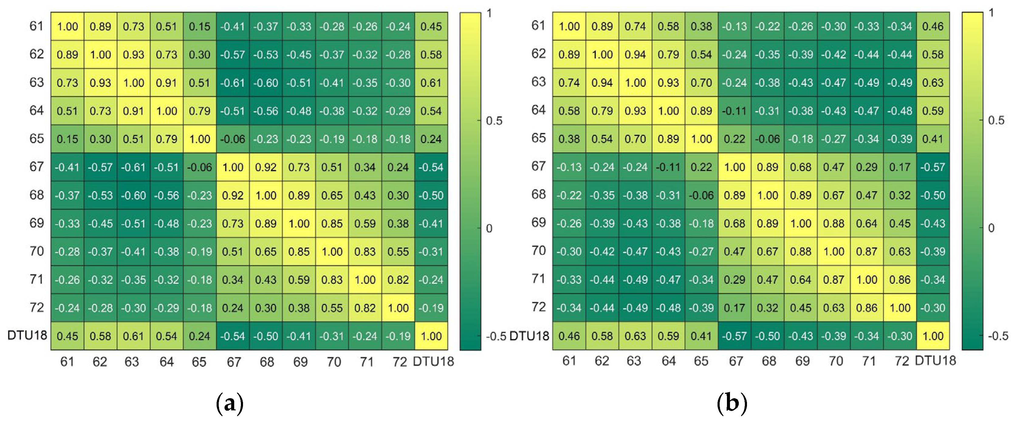
3.2.2. Feature Sensitivity Analysis

To further assess the contribution of the DW, IDW, DDMA, LES, specular point elevation (ELE), DDM signal-to-noise ratio (SNR), atmospheric delay (ATM), ocean wind speed (EAR5), and retracking algorithm (PCP, PCP70, and PFD) features to the SSH retrieval model, different combinations of the input parameters were designed as follows:

• Set 1: DW
• Set 2: IDW
• Set 3: IDW and ELE
• Set 4: IDW and SNR
• Set 5: IDW, ELE, and SNR
• Set 6: IDW, ELE, SNR, and ATM
• Set 7: IDW, ELE, SNR, and EAR5
• Set 8: IDW, ELE, SNR, ATM, and EAR5
• Set 9: IDW, ELE, SNR, ATM, EAR5, and LES
• Set 10: IDW, ELE, SNR, ATM, EAR5, and PCP
• Set 11: IDW, ELE, SNR, ATM, EAR5, and PFD
• Set 12: IDW, ELE, SNR, ATM, EAR5, and PCP70
• Set 13: DDMA, ELE, SNR, ATM, EAR5, and PCP
• Set 14: IDW, ELE, SNR, ATM, EAR5, LES, PCP, and DDMA

For verifying the robustness of the GSMHLFO, the random seed number of the 5-fold cross-validation was replaced twice. Changing the random seed number was equivalent to reslicing the training and validation sets. The performance indicators of the three experimental outcomes on the test set are summarized in

Table 2. Performance indicators of the GSMHLFO in different datasets.

Set	The First Experiment			The Second Experiment			The Third Experiment
	MAD (m)	RMSE (m)	PCC	MAD (m)	RMSE (m)	PCC	MAD (m)	RMSE (m)	PCC
Set 1	13.66	18.28	0.81	13.47	18.15	0.81	13.52	18.09	0.81
Set 2	11.90	17.05	0.85	11.73	16.95	0.85	11.82	16.83	0.85
Set 3	11.40	16.43	0.87	11.47	16.52	0.87	11.40	16.40	0.87
Set 4	11.65	16.66	0.87	11.59	16.62	0.87	11.66	16.9	0.87
Set 5	8.72	12.16	0.91	8.65	12.04	0.91	8.59	11.57	0.91
Set 6	5.54	7.79	0.97	5.67	7.85	0.97	5.59	7.82	0.97
Set 7	6.89	9.60	0.95	6.75	9.49	0.95	6.83	9.62	0.95
Set 8	4.86	6.96	0.97	4.82	6.90	0.97	4.85	6.96	0.97
Set 9	4.78	6.73	0.98	4.75	6.69	0.98	4.71	6.65	0.98
Set 10	4.73	6.67	0.97	4.76	6.71	0.97	4.75	6.69	0.97
Set 11	5.09	7.16	0.97	5.05	7.14	0.97	5.01	7.12	0.97
Set 12	5.15	7.21	0.97	5.11	7.18	0.97	5.09	7.15	0.97
Set 13	5.02	7.30	0.97	5.05	7.26	0.97	4.97	7.10	0.97
Set 14	4.23	5.94	0.98	4.32	6.05	0.98	4.18	5.91	0.98

. As seen in Table 2, the MAD, RMSE, and PCC of each model do not change appreciably in the three experiments.

From Set 1 and Set 2, it can be seen that the use of the IDW dataset can utilize more DDM information compared to the DW dataset, which results in better retrieval performance. The RMSE of the retrieval results is only slightly reduced after adding SNR and ELE characteristics alone, with no significant improvement (shown by Set 2, Set 3, and Set 4). However, the simultaneous addition of SNR and ELE features can significantly improve the retrieval precision of SSH, with PCC increasing by 7.1% and RMSE decreasing by 26.7% (shown by Set 2 and Set 5). Set 6 and Set 7 demonstrate that the features EAR5 and ATM can contribute positively to the SSH retrieval of the GSMHLFO l, with the enhancement of the ATM feature being particularly significant (relative to Set 5). Set 8 presents the retrieval results of SSH after adding both the EAR5 feature and the ATM feature. Compared to the feature Set 5, PCC increased by 6.6%, and RMSE decreased by 44.3%. This enhancement is mainly because the ATM feature can provide additional signal propagation path information, and the EAR5 feature provides additional sea surface roughness information. Feature Sets 9–12 analyze the effect of LES, PCP, PFD, and PCP70 features constructed from DDM on SSH retrieval. It can be seen that LES and PCP contribute positively to SSH retrieval (Sets 8–10), while PFD and PFD70 contribute negatively (shown by Sets 8, 11, and 12). Feature Set 13 utilizes DDMA instead of the entire IDW data, and it can be seen that the retrieval precision is slightly lower than using the entire IDW data (shown by Set 13 and Set 10). By adding all the positive contribution features as the input of the neural network (Set 14), the RMSE of the retrieval SSH can be improved to 4.23 m and the PCC to 0.98.

4. Results

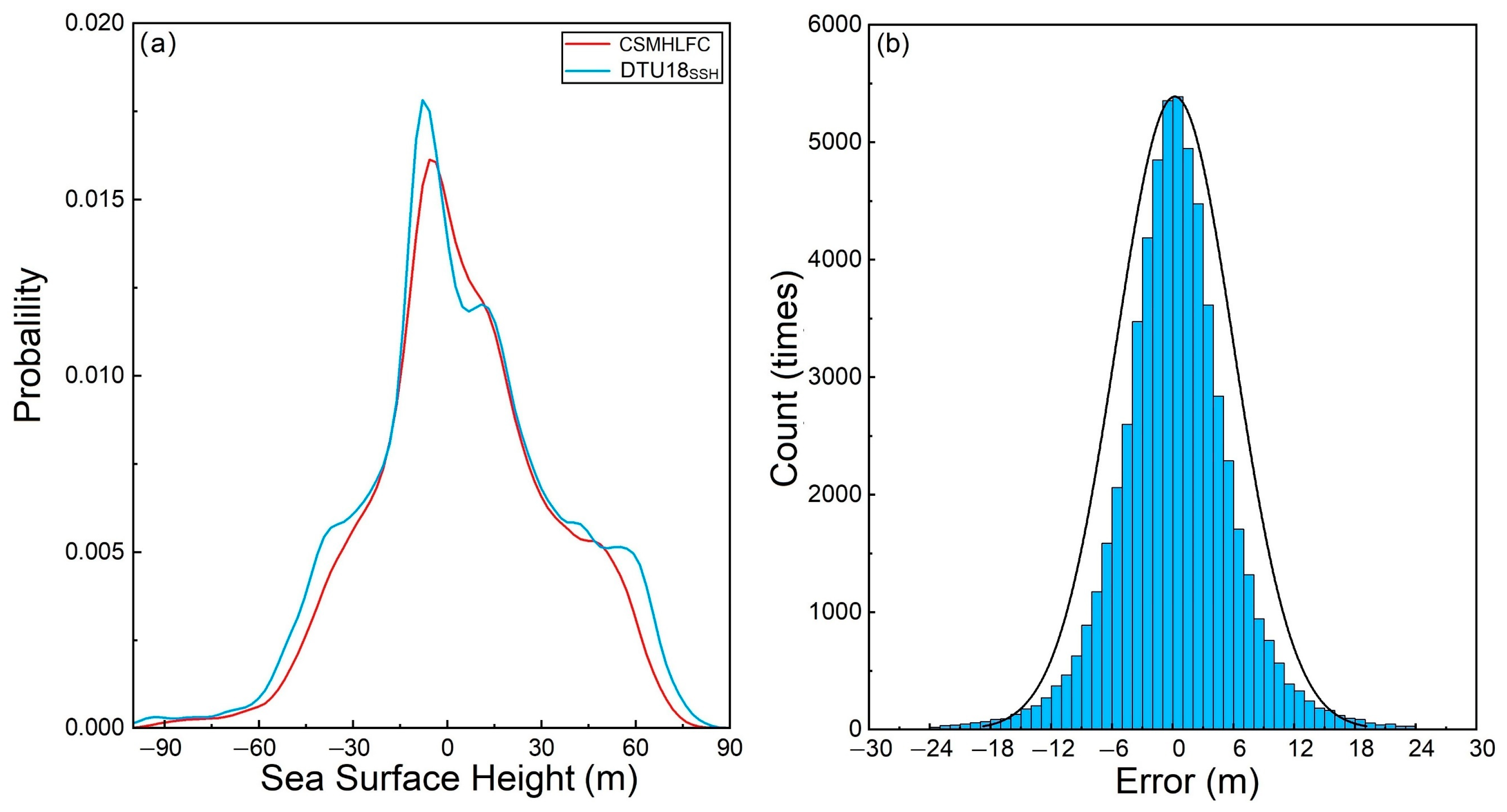
4.1. Analysis of SSH Retrieval Results

In this section, the SSH retrieval performance of the proposed GSMHLFO with four hidden layers and 200 neurons in each layer is evaluated. The SSH retrieval model was built by using Set 14 with the best retrieval precision in Section 3.2.2 as the input to the GSMHLFO. The GSMHLFO performance was evaluated with a completely blind test set.

The training and validation error profiles of the GSMHLFO are given in Figure 8a. It can be seen that at the early stage of training, both training and validation errors decrease significantly with the increase in the number of epochs. Additionally, the error gradually stabilizes after 400 epochs. Meanwhile, the RMSE on the validation set is slightly higher than that on the training set after the error function was stabilized. This is mainly because the model can use all of the samples from the training set for training, while the samples on the validation set are only used as feedback to adjust the parameters.

The scatter density plot between the retrieval results of the GSMHLFO and the SSH of the DTU18 validation model is given in Figure 8b. It can be intuitively seen that the retrieval results of the GSMHLFO have a strong correlation with the DTU18 verification model, with a PCC of 0.98. However, because TDS-1 is not designed for altimetry measurements, the satellite receiver was not optimized for altimetry. The results have a considerable retrieval error, with the MAD of 4.23 m and the RMSE of 5.94 m.

The probability density function (PDF) of the SSH of the GSMHLFO and the DTU18 verification model is shown in Figure 9a. It can be seen that the data distribution of SSH retrieved by the GSMHLFO is almost the same as that of the DTU18 verification model. However, the GSMHLFO retrievals have slightly lower PDF of SSH in the range of −10~0 m, −60~−20 m, and 45~90 m than the DTU18 validation model. This is mainly due to the uneven distribution of different SSHs in the training dataset. Figure 9b shows the error distribution histogram of the retrieval results of the GSMHLFO relative to the SSH of the DTU18 verification model. The statistical results are close to a normal distribution in which 69.78% of the retrieval errors are between −5 and 5 m, and 92.13% of the retrieval errors are between −10 and 10 m.

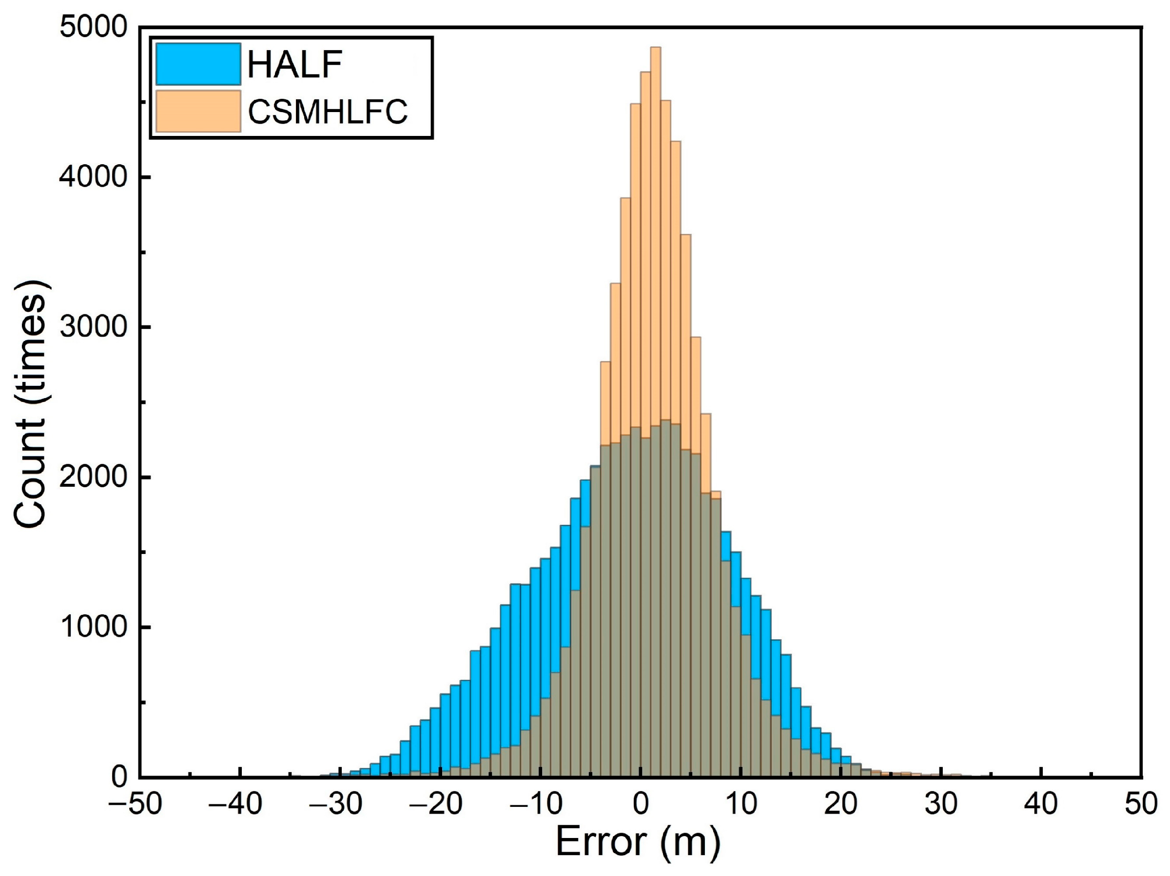
4.2. Evaluation of SSH Retrieval Results

We compared the retrieval precision of the two methods to verify the superiority of the GSMHLFO over the traditional spaceborne GNSS-R SSH retrieval method. In the conventional SSH retrieval, the time delay difference between the reflected signal and the direct signal was estimated using the HALF retracking method. A point on the leading edge of the correlation waveform at 70% of the maximum correlation power was chosen as the retracking point. Moreover, various errors in the time delay measurements were corrected by building the corresponding error models [46].

Table 3. Error factors and corresponding error correction methods.

Errors	Correction Method
Ionospheric delay	GIM
Tropospheric delay	UNB3m
Antenna baseline	Metadata
GPS orbit error	IGS Ephemeris
TDS-1 orbit error	Metadata
Delay error	Reflected Signal Geometry
TDS-1 data bias	Metadata
Tracking error noise	HALF

lists the various errors in the conventional SSH retrieval method and the related error correction methods [46]. Among them, ionospheric and tropospheric corrections were also used as input features for the model of GSMHLFO proposed in this paper (in Section 3.2). These provide additional information on the signal propagation path.

Figure 10a,b show the global SSH retrieval results of the traditional HALF retracking method and the GSMHLFO on the test set, respectively. Figure 10c shows the SSH of the corresponding DTU18 validation model. Figure 10 shows that both models have good retrieval results, and the resulting SSHs are globally consistent with the DTU18 validation model SSHs. Furthermore, in the red box, GSMHLFO exhibits better retrieval results with fewer errors with the DTU18 validation model compared to the traditional HALF retracking method. GSMHLFO can more accurately mine the relationship between the raw input data and SSH by increasing the information available to the DDM.

Figure 11 shows the error statistics of the global SSH retrieved by the HALF retracking method and the GSMHLFO when compared with DTU18 data. The retrieval results of the GSMHLFO are superior. The retrieval error of the GSMHLFO is smaller, and about 92.13% of the retrieval error is between −10 and 10 m, while the HALF retracing method is only 67.63%.

The precision indicators of the two models are quantitatively presented in

Table 4. Comparison of SSH retrieval performance between the GSMHLFO and HALF retracking method.

	MAD (m)	RMSE (m)	PCC
HALF	6.30	7.92	0.89
GSMHLFO	4.23	5.94	0.97
Improve (%)	32.86	25.00	8.99

. The GSMHLFO outperforms the traditional retracking algorithm in MAD, RMSE, and PCC precision metrics. The application of the GSMHLFO effectively improves the precision of SSH retrieval. The MAD and RMSE are reduced by 32.86% and 25.00%, respectively, and the PCC is improved by 8.99%.

5. Discussion

The retrieval results of the proposed GSMHLFO with four hidden layers and 200 neurons in each layer strongly correlate with the DTU18 validated model, with a PCC of 0.98. However, because TDS-1 is not designed for altimetry measurements, the satellite receiver has not been optimized for altimetry. The results have a considerable retrieval error, with a MAD of 4.23 m and an RMSE of 5.94 m. The main reasons for the error are: (1) For altimetry missions, TDS-1 L1B-level data suffer from limited delay resolution (224.3942 ns), narrow receiver bandwidth (~2 MHz), and low peak antenna gain (13.3 dB). (2) Since TDS-1 can only obtain L1 single-frequency measurement signals, atmospheric delay errors cannot be eliminated by dual-frequency measurements. (3) Some abnormal DDM data that have not been removed from the data will also affect the SSH retrieval results. The issues above will have an overall error of 3.5~7 m in the retrieval results [22,46]. After analyzing 14 feature sets with various information details, it can be observed that ELE, SNR, ATM, and EAR5 can make significant contributions to GSMHLFO-based SSH retrieval, while PFD and PFD70 provide negative contributions. Moreover, compared to the traditional HALF retracking method, the SSH retrieval algorithm based on the GSMHLFO can effectively improve the precision of SSH retrieval.

6. Conclusions

The traditional GNSS-R altimetry method has a more complicated error model and limited retrieval precision. To address this deficiency, in this research, we developed the GSMHLFO for SSH retrieval. The main research results can be summarized in the following points:

(1) The GSMHLFO is constructed by combining the MHL-NN, feature engineering, and grid search algorithm. First, the feature extraction method was used to downscale and optimize the original DW data. Second, the feature construction method was used to construct new features sensitive to SSH by analyzing the effects of signal propagation path, traditional retracking algorithm, and sea surface roughness. Third, the MHL-NN was used to build the SSH prediction model, and the number of hidden layers and neurons in each layer were optimized using the grid search algorithm.

(2) The retrieval results of the proposed GSMHLFO with four hidden layers and 200 neurons in each layer strongly correlate with the DTU18 validated model, with a PCC of 0.98. However, affected by the quality of the TDS-1 L1B data (limited delay resolution, low receiver bandwidth, and low antenna gain) and atmospheric delay error, the RMSE and MAD are equal to 5.94 and 4.23 m, respectively.

(3) After analyzing 14 feature sets with various information details, we observed that compared with the DW dataset, GSMHLFO trained by the IDW dataset can achieve better retrieval results. Moreover, the ELE, SNR, ATM, and EAR5 can provide significant contributions to the SSH retrieval based on GSMHLFO.

(4) Compared to the traditional HALF retracking method, the SSH retrieval algorithm based on the GSMHLFO can effectively improve the precision of SSH retrieval. The MAD and RMSE are reduced by 32.86% and 25.00%, respectively, while the PCC is improved by 8.99%.

The new MHL-NN model proposed in this study presents a new idea for the future GNSS-R ocean altimetry algorithm, which can precisely retrieve the global SSH. In addition, the work of this paper needs to be continuously improved. The proposed MHL-NN model can be further optimized by training on more extensive datasets. Furthermore, more physical parameters related to SSH can be explored to improve the retrieval precision.

References

1. Wang, J.; Xu, H.; Yang, L.; Song, Q.; Ma, C. Cross-calibrations of the HY-2B altimeter using Jason-3 satellite during the period of April 2019–September 2020. Front. Earth Sci. 2021, 9, 215–231. [Google Scholar] [CrossRef]
2. Liu, Z.; Zheng, W.; Wu, F.; Kang, G.; Sun, X.; Wang, Q. Relationship Between Altimetric Quality and Along-Track Spatial Resolution for iGNSS-R Sea Surface Altimetry: Example for the Airborne Experiment. Front. Earth Sci. 2021, 9, 213–222. [Google Scholar] [CrossRef]
3. Wu, F.; Zheng, W.; Liu, Z. Quantifying GNSS-R Delay Sea State Bias and Predicting Its Variation Based on Ship-Borne Observations in China’s Seas. IEEE Geosci. Remote Sens. Lett. 2022, 19, 1–5. [Google Scholar] [CrossRef]
4. Cui, Z.; Zheng, W.; Wu, F.; Li, X.; Zhu, C.; Liu, Z.; Ma, X. Improving GNSS-R Sea Surface Altimetry Precision Based on the Novel Dual Circularly Polarized Phased Array Antenna Model. Remote Sens. 2021, 13, 2974. [Google Scholar] [CrossRef]
5. Liu, Z.; Zheng, W.; Wu, F.; Cui, Z.; Kang, G. A Necessary Model to Quantify the Scanning Loss Effect in Spaceborne iGNSS-R Ocean Altimetry. IEEE J. Select. Top. Appl. Earth Obs. Remote Sens. 2021, 14, 1619–1627. [Google Scholar] [CrossRef]
6. D’Addio, S.; Martín-Neira, M.; Bisceglie, M.d.; Galdi, C.; Alemany, F.M. GNSS-R altimeter based on doppler multi-looking. IEEE J. Select. Top. Appl. Earth Obs. Remote Sens. 2014, 7, 1452–1460. [Google Scholar] [CrossRef]
7. Wu, F.; Zheng, W.; Li, Z.; Liu, Z. Improving the GNSS-R specular reflection point positioning accuracy using the gravity field normal projection reflection reference surface combination correction method. Remote Sens. 2019, 11, 33. [Google Scholar] [CrossRef] [Green Version]
8. Martin-Neira, M. A passive reflectometry and interferometry system (PARIS): Application to ocean altimetry. ESA J. 1993, 17, 331–355. [Google Scholar]
9. He, Y.; Gao, F.; Xu, T.; Meng, X.; Wang, N. Coastal altimetry using interferometric phase from GEO satellite in quasi-zenith satellite system. IEEE Geosci. Remote Sens. Lett. 2021, 19, 1–5. [Google Scholar] [CrossRef]
10. Cardellach, E.; Rius, A.; Martín-Neira, M.; Fabra, F.; Nogués-Correig, O.; Ribó, S.; Kainulainen, J.; Camps, A.; Addio, S.D. Consolidating the precision of interferometric GNSS-R ocean altimetry using airborne experimental data. IEEE Trans. Geosci. Remote Sens. 2014, 52, 4992–5004. [Google Scholar] [CrossRef]
11. Wang, Q.; Zheng, W.; Wu, F.; Xu, A.; Zhu, H.; Liu, Z. A new GNSS-R altimetry algorithm based on machine learning fusion model and feature optimization to improve the precision of sea surface height retrieval. Front. Earth Sci. 2021, 9, 123–135. [Google Scholar] [CrossRef]
12. Sun, X.; Zheng, W.; Wu, F.; Liu, Z. Improving the iGNSS-R Ocean Altimetric Precision Based on the Coherent Integration Time Optimization Model. Remote Sensing 2021, 13, 4715. [Google Scholar] [CrossRef]
13. Mashburn, J.; Axelrad, P.; Lowe, S.T.; Larson, K.M. Global ocean altimetry with GNSS reflections from TechDemoSat-1. IEEE Trans. Geosci. Remote Sens. 2018, 56, 4088–4097. [Google Scholar] [CrossRef]
14. Li, W.; Cardellach, E.; Fabra, F.; Ribó, S.; Rius, A. Assessment of spaceborne GNSS-R ocean altimetry performance using CYGNSS mission raw data. IEEE Trans. Geosci. Remote Sens. 2020, 58, 238–250. [Google Scholar] [CrossRef]
15. Mashburn, J.; Axelrad, P.; Zuffada, C.; Loria, E.; O’Brien, A.; Haines, B. Improved GNSS-R ocean surface altimetry with CYGNSS in the seas of indonesia. IEEE Trans. Geosci. Remote Sens. 2020, 58, 6071–6087. [Google Scholar] [CrossRef]
16. Liu, Z.; Zheng, W.; Wu, F.; Kang, G.; Li, Z.; Wang, Q.; Cui, Z. Increasing the Number of Sea Surface Reflected Signals Received by GNSS-Reflectometry Altimetry Satellite Using the Nadir Antenna Observation Capability Optimization Method. Remote Sens. 2019, 11, 2473. [Google Scholar] [CrossRef] [Green Version]
17. Wu, F.; Zheng, W.; Liu, Z.; Sun, X. Improving the Specular Point Positioning Accuracy of Ship-borne GNSS-R Observations in China’s Seas based on a new Instantaneous Sea Reflection Surface Model. Front. Earth Sci. 2021, 9, 112–122. [Google Scholar] [CrossRef]
18. Li, Z.; Zuffada, C.; Lowe, S.T.; Lee, T.; Zlotnicki, V. Analysis of GNSS-R altimetry for mapping ocean mesoscale sea surface heights using high-resolution model simulations. IEEE J. Sel. Top. Appl. Earth Obs. Remote Sens. 2016, 9, 4631–4642. [Google Scholar] [CrossRef]
19. Li, W.; Rius, A.; Fabra, F.; Cardellach, E.; Martin-Neira, M. Revisiting the GNSS-R waveform statistics and its impact on altimetric retrievals. IEEE Trans. Geosci. Remote Sens. 2018, 56, 2854–2871. [Google Scholar] [CrossRef]
20. Clarizia, M.P.; Ruf, C.; Cipollini, P.; Zuffada, C. First spaceborne observation of sea surface height using GPS-reflectometry. Geophys. Res. Lett. 2016, 43, 767–774. [Google Scholar] [CrossRef] [Green Version]
21. Jing, C.; Niu, X.; Duan, C.; Lu, F.; Yang, X. Sea surface wind speed retrieval from the first chinese GNSS-R mission: Technique and preliminary results. Remote Sens. 2019, 11, 3013. [Google Scholar] [CrossRef] [Green Version]
22. Xu, L.; Wan, W.; Chen, X.; Zhu, S.; Hong, Y. Spaceborne GNSS-R observation of global lake level: First results from the TechDemoSat-1 mission. Remote Sens. 2019, 11, 1438. [Google Scholar] [CrossRef] [Green Version]
23. Reynolds, J.; Clarizia, M.P.; Santi, E. Wind speed estimation from CYGNSS using artificial neural networks. IEEE J. Sel. Top. Appl. Earth Obs. Remote Sens. 2020, 13, 708–716. [Google Scholar] [CrossRef]
24. Li, X.; Yang, D.; Yang, J.; Zheng, G.; Han, G.; Nan, Y.; Li, W. Analysis of coastal wind speed retrieval from CYGNSS mission using artificial neural network. Remote Sens. Environ. 2021, 260, 112454–112466. [Google Scholar] [CrossRef]
25. Liu, Y.; Collett, I.; Morton, Y.J. Application of neural network to GNSS-R wind speed retrieval. IEEE Trans. Geosci. Remote Sens. 2019, 57, 9756–9766. [Google Scholar] [CrossRef]
26. Chu, X.; He, J.; Song, H.; Qi, Y.; Sun, Y.; Bai, W.; Li, W.; Wu, Q. Multimodal deep learning for heterogeneous GNSS-R data fusion and ocean wind speed retrieval. IEEE J. Sel. Top. Appl. Earth Obs. Remote Sens. 2020, 13, 5971–5981. [Google Scholar] [CrossRef]
27. Luo, L.; Bai, W.; Sun, Y.; Xia, J. GNSS-R sea surface wind speed inversion based on tree model machine learning method. Chin. J. Space Sci. 2020, 40, 595–601. [Google Scholar] [CrossRef]
28. Jia, Y.; Jin, S.; Savi, P.; Gao, Y.; Tang, J.; Chen, Y.; Li, W. GNSS-R soil moisture retrieval based on a XGboost machine learning aided method: Performance and validation. Remote Sens. 2019, 11, 1655. [Google Scholar] [CrossRef] [Green Version]
29. Yan, Q.; Huang, W. Sea ice sensing from GNSS-R data using convolutional neural networks. IEEE Geosci. Remote Sens. Lett. 2018, 15, 1510–1514. [Google Scholar] [CrossRef]
30. Wu, F.; Zheng, W.; Li, Z.; Liu, Z. Improving the positioning accuracy of satellite-borne GNSS-R specular reflection point on sea surface based on the ocean tidal correction positioning method. Remote Sens. 2019, 11, 1626. [Google Scholar] [CrossRef] [Green Version]
31. Yuan, J.; Guo, J.; Niu, Y.; Zhu, C.; Li, Z. Mean sea surface model over the sea of Japan determined from multi-satellite altimeter data and tide gauge records. Remote Sens. 2020, 12, 4168. [Google Scholar] [CrossRef]
32. Egbert, G.D.; Erofeeva, S.Y. Efficient inverse modeling of barotropic ocean tides. J. Atmos. Ocean. Technol. 2002, 19, 183–204. [Google Scholar] [CrossRef] [Green Version]
33. Wessel, P.; Smith, W. A global self-consistent, hierarchical, high-resolution shoreline. J. Geophys. Res. 1996, 101, 8741–8743. [Google Scholar] [CrossRef] [Green Version]
34. Tian, Y. Research on Spaceborne Multimode GNSS Reflectometry Sea Wind Sensing Signal Processing; National Space Science Center, Chinese Academy of Sciences: Beijing, China, 2021. [Google Scholar]
35. Hu, C.; Benson, C.; Park, H.; Camps, A.; Rizos, C. Detecting targets above the earth’s surface using GNSS-R delay doppler maps: Results from TDS-1. Remote Sens. 2019, 11, 2327. [Google Scholar] [CrossRef] [Green Version]
36. Garrison, J.L. A statistical model and simulator for ocean-reflected GNSS signals. IEEE Trans. Geosci. Remote Sens. 2016, 54, 6007–6019. [Google Scholar] [CrossRef]
37. Liu, L.; Sun, Y.; Bai, W.; Luo, L. The inversion of sea surface wind speed in GNSS-R base on the model fusion of data mining. Geomat. Inf. Sci. Wuhan Univ. 2020, 12, 1–10. [Google Scholar] [CrossRef]
38. Jung, Y. Multiple predicting K-fold cross-validation for model selection. J. Nonparametric Stat. 2018, 30, 197–215. [Google Scholar] [CrossRef]
39. Lavalle, S.M.; Branicky, M.S.; Lindemann, S.R. On the Relationship between Classical Grid Search and Probabilistic Roadmaps. Int. J. Rob. Res. 2004, 23, 673–692. [Google Scholar] [CrossRef]
40. Clarizia, M.P.; Ruf, C.S. Wind speed retrieval algorithm for the cyclone global navigation satellite system (CYGNSS) mission. IEEE Trans. Geosci. Remote Sens. 2016, 54, 4419–4432. [Google Scholar] [CrossRef]
41. Rodgers, J.L.; Nicewander, W.A. Thirteen ways to look at the correlation coefficient. Am. Stat. 1988, 42, 59–66. [Google Scholar] [CrossRef]
42. Clarizia, M.P.; Ruf, C.S.; Jales, P.; Gommenginger, C. Spaceborne GNSS-R minimum variance wind speed estimator. IEEE Trans. Geosci. Remote Sens. 2014, 52, 6829–6843. [Google Scholar] [CrossRef]
43. Hernández-Pajares, M.; Juan, J.; Sanz, J.; Orus, R.; Garcia-Rigo, A.; Feltens, J.; Komjathy, A.; Schaer, S.; Krankowski, A. The IGS VTEC maps: A reliable source of ionospheric information since 1998. J. Geod. 2008, 83, 263–275. [Google Scholar] [CrossRef]
44. Yan, Z.; Zheng, W.; Wu, F.; Wang, C.; Zhu, H.; Xu, A. Correction of Atmospheric Delay Error of Airborne and Spaceborne GNSS-R Sea Surface Altimetry. Front. Earth Sci. 2022, 10, 223–234. [Google Scholar] [CrossRef]
45. Leandro, R.; Santos, M.; Langley, R.B. UNB neutral atmosphere models: Development and performance. In Proceedings of the National Technical Meeting of the Institute of Navigation, Monterey, CA, USA, 18–20 January 2006; pp. 564–573. [Google Scholar] [CrossRef] [Green Version]
46. Mashburn, J.R. Analysis of GNSS-R Observations for Altimetry and Characterization of Earth Surfaces; University of Colorado: Boulder, CO, USA, 2018. [Google Scholar]
Figure 1. DDM with different reflective surfaces. (a) DDM with sea surface reflection; (b) DDM with sea ice reflection; (c) DDM with land edge reflection; (d) DDM with noise.
Remotesensing 14 03161 g001
Figure 2. Statistical results of the time delay and Doppler pixel position where the peak power of DDM data is located.
Remotesensing 14 03161 g002
Figure 3. Global distribution of SSH (m) of TDS-1 experimental data.
Remotesensing 14 03161 g003
Figure 4. Schematic diagram of ANN structure.
Remotesensing 14 03161 g004
Figure 5. Hyperparameter preference results. (a) RMSE of the retrieved SSH for the GSMHLFO with different hidden layers and the number of neurons in each layer; (b) PCC of the retrieved SSH for the GSMHLFO with different hidden layers and the number of neurons in each layer.
Remotesensing 14 03161 g005
Figure 6. Calculation regions for the noise floor and DDMA. (a) The area used to calculate the noise floor; (b) the area used to calculate DDMA.
Remotesensing 14 03161 g006
Figure 7. Correlation heatmap. (a) Heat map of PCC between DW and DTU18 SSH (m); (b) Heat map of PCC between IDW and DTU18 SSH (m).
Remotesensing 14 03161 g007
Figure 8. The retrieval results of the GSMHLFO. (a) Training and validation error profiles of the GSMHLFO; (b) Scatter density plots of the retrieval results of the GSMHLFO.
Remotesensing 14 03161 g008
Figure 9. Error statistics results of the GSMHLFO. (a) PDF plot of the retrieval results of the GSMHLFO relative to the DTU18 validation data; (b) Histogram of the error distribution of the retrieval results of the GSMHLFO.
Remotesensing 14 03161 g009
Figure 10. Global SSH of different models. (a) Global SSH retrieval results of HALF conventional method; (b) Global SSH retrieval results of the GSMHLFO; (c) Global SSH of DTU18 validation model. The red box compares the difference in SSH between the three models HALF, GSMHLFO and DTU18.
Remotesensing 14 03161 g010
Figure 11. Global SSH error statistics were obtained by the HALF retracking method and the GSMHLFO.
Remotesensing 14 03161 g011