Article

Evaluation of Vegetation Indexes and Green-Up Date Extraction Methods on the Tibetan Plateau

1
Key Laboratory of Geographic Information Science, Ministry of Education, East China Normal University, Shanghai 200241, China
2
School of Geographic Sciences, East China Normal University, Shanghai 200241, China
3
Key Laboratory of Spatial-Temporal Big Data Analysis and Application of Natural Resources in Megacities, Ministry of Natural Resources, Shanghai 200241, China
4
State Key Laboratory of Earth Surface Processes and Resource Ecology, Beijing Normal University, Beijing 100875, China
5
Department of Geography and Planning, Appalachian State University, Boone, NC 28608, USA
*
Author to whom correspondence should be addressed.
Remote Sens. 2022, 14(13), 3160; https://doi.org/10.3390/rs14133160
Submission received: 20 May 2022 / Revised: 24 June 2022 / Accepted: 28 June 2022 / Published: 1 July 2022

Abstract

:
The vegetation green-up date (GUD) of the Tibetan Plateau (TP) is highly sensitive to climate change. Accurate estimation of GUD is essential for understanding the dynamics and stability of terrestrial ecosystems and their interactions with climate. The GUD is usually determined from a time-series of vegetation indices (VIs). The adoption of different VIs and GUD extraction methods can lead to different GUDs. However, our knowledge of the uncertainty in these GUDs on TP is still limited. In this study, we evaluated the performance of different VIs and GUD extraction methods on TP from 2003 to 2020. The GUDs were determined from six Moderate Resolution Imaging Spectroradiometer (MODIS) derived VIs: normalized difference vegetation index (NDVI), enhanced vegetation index (EVI), normalized difference infrared index (NDII), phenology index (PI), normalized difference phenology index (NDPI), and normalized difference greenness index (NDGI). Four extraction methods (βmax, CCRmax, G20, and RCmax) were applied individually to each VI to determine GUD. The GUDs obtained from all VIs showed similar patterns of early green-up in the eastern and late green-up in the western plateau, and similar trend of GUD advancement in the eastern and postponement in the western plateau. The accuracy of the derived GUDs was evaluated by comparison with ground-observed GUDs from 19 agrometeorological stations. Our results show that two snow-free VIs, NDGI and NDPI, had better performance in GUD extraction than the snow-calibrated conventional VIs, NDVI and EVI. Among all the VIs, NDGI gave the highest GUD accuracy when combined with the four extraction methods. Based on NDGI, the GUD extracted by the CCRmax method was found to have the highest consistency (r = 0.62, p < 0.01, RMSE = 11 days, bias = −3.84 days) with ground observations. The NDGI also showed the highest accuracy for preseason snow-covered site-years (r = 0.71, p < 0.01, RMSE = 10.69 days, bias = −4.05 days), indicating its optimal resistance to snow cover influence. In comparison, NDII and PI hardly captured GUD. NDII was seriously affected by preseason snow cover, as indicated by the negative correlation coefficient (r = −0.34, p < 0.1), high RMSE and bias (RMSE = 50.23 days, bias = −24.25 days).

1. Introduction

The Tibetan Plateau (TP), located in southwest China and central Asia, is the highest and largest plateau in the world. The special geographical conditions, unique natural environment, and fragile alpine ecosystem of the TP make it a region susceptible to climate change [1]. In the past 50 years, the temperature on the TP has risen by an average of approximately 0.37 °C per decade, twice more than the global average ascending rate during the same period [2]. Climate change often leads to acute changes in plant growth and generates a great instability in ecosystem. A sensitive indicator of terrestrial ecosystem response to climate change is vegetation phenology. In particular, the vegetation green-up date (GUD)—which refers to the time when vegetation photosynthetic activity and plant germination and growth processes under suitable hydrothermal conditions begin—describes the initial increase in land surface greenness in spring [3]. GUD changes can affect the interaction between biosphere and atmosphere, thereby influencing carbon, water, and energy balance [4,5,6]. Therefore, GUD is one of the most important parameters for studying the response and feedback mechanisms of terrestrial ecosystems to climate change (e.g., [7,8]).
Traditionally, GUD detection relies on ground-based observations, such as field visual observations and near-surface measurements. Field visual observations directly observe the seasonality and interannual variation of vegetation phenological growth rhythm at fixed stations. This method is time-consuming and labor-intensive, and is limited by time, place, and species factors. Near-surface measurements record vegetation information by instruments mounted on platforms such as tripod and unmanned aerial vehicle, including optical digital camera [9], multi-band spectroradiometer [10], and CO2 flux sensor [11]. Digital camera and spectroradiometer can obtain vegetation phenological information at canopy level [12], while CO2 flux measurements provide gross primary production, from which the detected GUD representing the “physiological phenology” of the vegetation can be found [13]. Despite their ability to observe vegetation information more efficiently, these methods are limited to a small spatial scale [14]. With satellite remote sensing data being available on a long-term global basis, estimates of GUD can be made on a large scale with high spatial and temporal resolution. Time series of vegetation indexes (VIs) are usually used for satellite-based GUD extraction. The normalized difference vegetation index (NDVI) is sensitive to canopy structure and chlorophyll and has been the most widely used VI [15]. However, NDVI can be influenced by the radiance from atmosphere and soil background, and is prone to saturation at a high leaf area index [16]. The enhanced vegetation index (EVI) improves the sensitivity in high biomass regions and reduces the effect from atmosphere and soil [17]. However, it is subject to topography [18]. Additionally, NDVI and EVI can increase with both vegetation growth and snow melt in spring, so the GUD estimation may be influenced by snow melt [19]. In order to account for the snow melt effect, several VIs have been proposed. The normalized difference infrared index (NDII) is expected to separate the two natural processes, as it increases with vegetation growth and decreases with snow melt [20]. However, NDII is ineffective for capturing GUD in places where the two processes occur simultaneously [21] and in some burned areas [22]. The phenology index (PI) combines NDVI and NDII to remove the confounding effects of brightness and wetness [21]. However, it cannot identify sparse vegetation [23,24], and thus it may struggle to recognize the initial growth of vegetation. The normalized difference phenology index (NDPI) is designed for deciduous ecosystems to best distinguish vegetation from soil and snow, while minimizing differences between these background components [24]. However, NDPI ignores the spectral properties of dry grass. By contrast, the normalized difference greenness index (NDGI) not only captures the presence of sparse vegetation well, but also compensates for the effect of dry grass on GUD extraction [23]. Its application is limited to tundra and grassland ecosystems. In large spatial scales, no matter which VI is used, the estimated GUD may have uneven distribution of accuracy due to the spatial heterogeneity of latitudes and vegetation types [25,26]. It is still unclear how these VIs perform in GUD extraction on the TP.
In addition, different GUD extraction methods also play important roles for identifying GUD from time series of VI values. These GUD extraction methods mainly fall into two categories: threshold-based methods and change detection methods [27]. The threshold-based methods include absolute threshold method [28] using a fixed VI value and relative threshold method [29,30] using a certain ratio of the amplitude of the VI curve to determine the GUD. Commonly used relative thresholds include 10% (G10), 20% (G20), and 50% (G50). Despite being simple and convenient, threshold-based methods have little practical biophysical significance. A single threshold is not universally applicable for GUD detection in a large region with different environmental conditions and vegetation types [31]. The absolute threshold method is susceptible to VI fluctuation caused by external factors instead of vegetation, resulting in the bias of GUD detection. In contrast, the relative threshold method excels at adaptability in GUD estimation due to its consideration of the differences between vegetation types and the annual variation in vegetation growth. However, the relative threshold method is sensitive to noise and may be unstable over time [29]. The change detection methods determine GUD by finding the change characteristic points on VI curve, such as the maximum value of the first derivative (βmax) [32], the first local maximum curvature change rate (CCRmax) of the annual VI curve [3], and the fastest change rate (RCmax) of multi-year averaged VI curve [33]. These change detection methods were regarded as effective in GUD extraction for general vegetation types and mixed vegetation pixels [34]. However, these change detection methods cannot accurately determine GUD if there is no abrupt VI increase during the growth stage, especially when the VI data were contaminated by cloud [35], or if the vegetation has no much seasonal spectral variation [36]. Furthermore, the change detection methods are also sensitive to the noise in VI time series [37]. In recent years, more effort has been made to develop the methods for deriving physiological GUD of specific vegetation types, especially for crops. For example, Pan et al. [38] extracted GUDs of corn and wheat based on the threshold with the highest probability of VI ratio. Xu et al. [39] calibrated the program of GUD estimations for barley, rape, wheat, and beet, by optimizing the smoothing method, algorithm of Best Index Slope Extraction, and the threshold setting based on ground-observed GUDs. These methods are actually the extensions of the threshold-based methods using empirical knowledge and statistical analysis. They are, to some extent, influenced by individual experience, and the correct and rational threshold for unbiased GUD estimation is difficult to define. Additionally, the phenology matching method was designed to match the ground-observed GUD to a certain trajectory feature point in the VI time series [37]. However, the GUD accuracy may be impacted by the considerable variability of ground observations across different years and locations [40]. Although these advanced methods have achieved some effectiveness in small field-scale areas and specific species, they have no widespread applicability. In contrast, the general GUD extraction methods (such as βmax, CCRmax, G20, and RCmax) are more suitable for large geographic areas such as TP.
Some studies have compared the performances of different GUD extraction methods, but most are limited to the analysis of a single conventional VI. White et al. [41] assessed ten GUD extraction methods in North America using NDVI data and found that individual methods differed in GUD estimates by ±60 days. Based on NDVI data, Wang et al. [42] employed five methods (RCmax, G20, G50, maximum relative change, and maximum increase) to extract GUD in China’s temperate monsoon area. They concluded that the GUD derived from G50 was significantly correlated with ground-observed GUD. Zhang et al. [43] evaluated three relative threshold methods (G10, G30, and G50), five absolute threshold methods (0.1, 0.5, 1, 1.5, and 2), and seasonal trend decomposition by loess in phenology extraction in China using the leaf area index and found that G10 gave a better GUD prediction than the other methods. Although previous studies have confirmed the non-negligible influences of extraction methods on GUD estimation, further research is needed to quantify the uncertainty of GUD determined from different VIs and by different methods.
This study evaluated the effects of VIs and extraction methods on the determination of GUD over the TP. We calculated GUDs based on the time series (2003–2020) of NDVI, EVI, NDII, PI, NDPI, and NDGI derived from Moderate Resolution Imaging Spectroradiometer (MODIS) surface reflectance data. Four GUD extraction methods (βmax, CCRmax, G20, and RCmax) were applied individually to each VI. We analyzed the spatiotemporal variation in GUDs derived from six VIs on the TP during the study period. By comparison with ground-observed GUD from 19 agrometeorological stations, we then evaluated the overall accuracy of GUDs derived from six VIs and their accuracy in areas with and without preseason snow cover. Based on the optimal VI, we also assessed the consistency of the GUDs extracted using different extraction methods with the ground observations. Then, we discussed the applicability of snow-free VIs on the TP and the impact of extraction methods on GUD accuracy.

2. Study Area and Data Sources
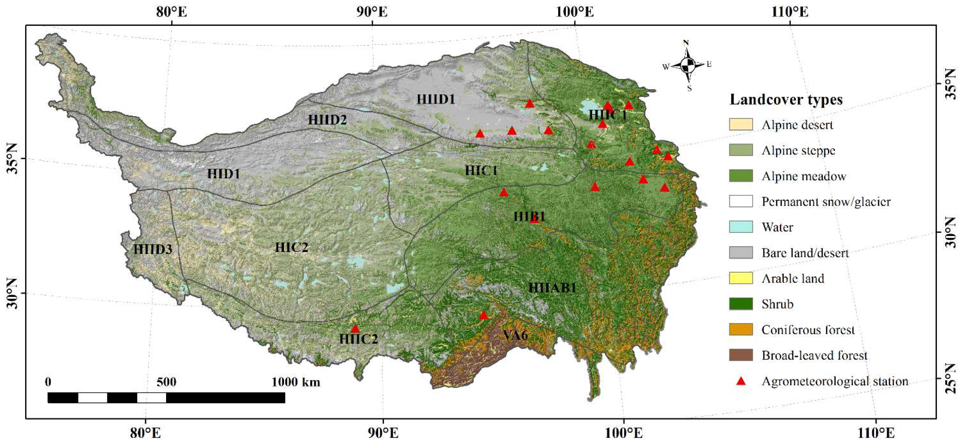
2.1. Study Area

The TP lies in southwestern China. Starting from the Pamir Plateau in the west, it reaches the Hengduan Mountains in the east, the southern margin of the Himalayas in the south, and the northern side of the Kunlun and Qilian Mountains in the north (26°00′12″N–39°46′50″N, 73°18′52″E–104°46′59″E; Figure 1). It covers an area of approximately 2.5 × 10⁶ km2 with an average elevation exceeding 4000 m above sea level (asl). The topography of the TP is complex, and its elevation gradually decreases from west to east and from north to south. The climate of the TP is characterized by low temperatures, little rainfall, and strong solar radiation. In general, it varies gradually from dry and cold in the northwest to humid and warm in the southeast [44].
These unique environmental conditions have formed a typical alpine ecosystem on the TP, where the vegetation distribution includes alpine-steppes and meadows over the flat plateau, shrubs in the valleys, and a small percentage of forest in the southeastern plateau (Figure 1). The vegetation growing season in the TP is mainly from May to September. According to topographical, moisture, and thermal features, the TP is divided into 11 eco-geographical regions [45] (Figure 1, Table A1).
The TP is also rich in snow in the winter season. The duration of snow cover varies across different elevation ranges and generally increases with altitude [46]. Higher elevations on the TP are covered perennially with snow.

2.2. Data Sources

2.2.1. Land Surface Reflectance Products

The Version 6, 8-day composite MODIS Terra surface reflectance MOD09A1 with a spatial resolution of 500 m over the TP from 2003 to 2020 was obtained from the USGS EarthExplorer (https://espa.cr.usgs.gov/, accessed on 13 December 2020). MODIS measured surface spectral reflectance at bands 1 to 7, and corrected for the effects of atmospheric conditions such as thin cirrus clouds, aerosols, Rayleigh scattering, etc. [47]. The following bands, red (band 1), near-infrared (NIR, band 2), blue (band 3), green (band 4), and short-wave infrared (SWIR, band 6), were employed to calculate the six VIs (NDVI, EVI, NDII, PI, NDPI, and NDGI).
For all the time series of VIs over the study area, the maximum value composite (MVC) method [48] was applied to synthesize every two consecutive 8-day composite VIs into 16-day composited VIs. This operation helped to eliminate data noise caused by cloud pollution and harsh atmospheric conditions. The VI time series was constructed using the date of the first day of each 16-day cycle from the MODIS product. The remaining missing data in the time series of the VIs were filled using linear interpolation. The Savitzky-Golay filter [49,50] was used to remove outliers and smoothen the time series.
To concentrate on pixels with seasonal vegetation dynamics, we used the following process, as recommended by Shen et al. [51]. Since the NDVI and EVI values of snow cover are lower than those of vegetation [52], for each pixel, we replaced the snow-polluted NDVI (or EVI) values with the median of the unpolluted winter NDVI or EVI values from November to March [51]. Pixels with snow cover were recognized by using the snow flag in the product quality evaluation data (MOD09A1). Pixels that met the following requirements were reserved: (1) the annual maximum NDVI occurred in the period between July and September, (2) the average NDVI from June to September exceeded 0.1, and (3) the average NDVI from July to September was 1.2 times higher than that from November to March [51]. According to the pixels retained by the above practices, we also selected pixels of EVI, NDII, PI, NDPI, and NDGI in the corresponding positions.

2.2.2. Ground-Observed GUD Data

The ground-observed GUD records for the TP during 2003–2013 were collected from the China Meteorological Data Sharing Service System (http://data.cma.cn/, accessed on 11 July 2021). The dataset contained observations from 19 agrometeorological stations. The dates of phenological phases with names of green-up (or emergence of seeding) in the dataset were used to represent the GUD. If there was more than one GUD record for any ground station in a year, the averaged GUD was used.

2.2.3. Snow Cover Product

The 500 m resolution daily and gapless snow cover product from 1 October 2002 to 30 September 2020 was produced for the TP using the HMRF modeling technique [53]. The HMRF modeling technique combined spectral, spatiotemporal, and environmental information in an optimal manner. This method can not only fill the data gaps in the original snow cover products but also significantly improve the accuracy of the original product. The overall accuracy of the data was verified to be 98.31% according to the snow depth data from ground meteorological stations, and 92.44% according to the snow cover extent extracted from Landsat-8 [54]. This snow cover product was used to determine the snow cover end date (SCED) for the study period, and to distinguish whether there is preseason snow cover at agrometeorological stations.

2.2.4. Land Cover Type Data

The land cover type map for the TP with a spatial resolution of 500 m was obtained from the Science Data Bank (http://www.scidb.cn/doi/10.11922/sciencedb.398, accessed on 15 July 2021). These data delineate the spatial distribution of main vegetation types on the TP, including alpine steppes, meadows, shrubs, and forests.

3. Methods

Six VIs (NDVI, EVI, NDII, PI, NDPI, and NDGI) were first calculated from MODIS surface reflectance products MOD09A1.The GUDs were then extracted using four methods (βmax, CCRmax, G20, and RCmax) for each VI. SCED was calculated from daily snow cover data to distinguish the areas with and without preseason snow cover. The Theil-Sen non-parametric regression was used to analyze the trend of GUD temporal variation. Then, the performances of different VIs and GUD extraction methods were assessed using Pearson’s correlation, linear regression, RMSE, and bias.

3.1. Calculation of VIs

3.1.1. NDVI

The NDVI is calculated as the normalized form of the red ( ρ R e d ) and NIR ( ρ N I R ) band reflectance [15]:
NDVI = ρ N I R ρ R e d ρ N I R + ρ R e d

3.1.2. EVI

The EVI adds a blue band ( ρ B l u e ) to enhance vegetation signals and correct the effects of soil background and aerosol scattering. It can improve sensitivity in areas with high biomass [17]:
EVI = 2.5 × ρ N I R ρ R e d ρ N I R + 6 × ρ R e d 7.5 × ρ B l u e + 1

3.1.3. NDII

NDII is the normalized composition of the NIR ( ρ N I R ) and SWIR band reflectance ( ρ S W I R ) [55]:
NDII = ρ N I R ρ S W I R ρ N I R + ρ S W I R

3.1.4. PI

The PI combines NDVI and NDII to solve the mixed effects of brightness and humidity on vegetation information [21]:
PI = { 0 , i f   NDVI   o r   NDII < 0 NDVI 2 NDII 2 0 , i f   PI < 0

3.1.5. NDPI

The NDPI utilizes the red, NIR and SWIR bands to significantly distinguish vegetation from background components (soil and snow) [24]:
NDPI = ρ N I R [ α × ρ R e d + ( 1 α ) × ρ S W I R ] ρ N I R + [ α × ρ R e d + ( 1 α ) × ρ S W I R ]
where α is a weight coefficient determined by the spectral configuration of satellite sensor, and ranges from 0.0 to 1.0. It was parameterized as 0.74 for MODIS bandwidths [24].

3.1.6. NDGI

The semi-analytical index NDGI consists of green, red, and NIR bands, to account for the spectral characteristics of soil, snow, dry grass, and vegetation, and it adopts a linear spectral mixture model to improve the ability of monitoring vegetation phenology [23]. NDGI is calculated as:
NDGI = α × ρ G r e e n + ( 1 α ) × ρ N I R ρ R e d α × ρ G r e e n + ( 1 α ) × ρ N I R + ρ R e d
where α is the weight coefficient that depends on the observation sensor. For MODIS data, α was found to be 0.65 in reference to Yang et al. [23].

3.2. Determination of Vegetation GUD

The GUD varies with different extraction methods, and its accuracy may have spatial heterogeneity [26]. Presently, there is no consensus on which method is best suited for the GUD extraction for different ecosystems [56]. In our study, four methods were employed to determine GUD from annual VI time series, including βmax, CCRmax, G20, and RCmax.
For the βmax, CCRmax, and G20 methods, the four-parameter logistic function was first used to fit the VI time series from the beginning of the year to the annual maximum VI [3]:
VI ( t ) = c 1 + e a + b t + d
where t is the time in days of year (DOY), VI ( t ) is the VI value at time t, a and b are fitting parameters, d is the initial background VI value, and c + d is the annual maximum VI value [3].
For RCmax, the VI time series from January to September of each year was fitted using a sixth-order polynomial.
Then, the mutation points on the fitting curves were determined as GUD with the following rules.

3.2.1. Method 1: βmax

This method focuses on the rate of increase in the VIs during the growing season, which is represented by the first derivative (β) of the fitted logistic function. The GUD is defined as the time at which β reaches its maximum [32].

3.2.2. Method 2: CCRmax

CCRmax calculates the curvature change rate (CCR) of the fitted logistic function as follows [3]:
CCR = b 3 c z { 3 z ( 1 z ) ( 1 + z ) 3 [ 2 ( 1 + z ) 3 + b 2 c 2 z ] [ ( 1 z ) 4 + ( b c z ) 2 ] 2.5 ( 1 + z ) 2 ( 1 + 2 z 5 z 2 ) [ ( 1 + z ) 4 + ( b c z ) 2 ] 1.5 }
where the meanings of a, b, and c are the same as those in Equation (7), z = e a + b t . The time corresponding to the first local maximum of CCR marks the GUD [3].

3.2.3. Method 3: G20

For G20, GUD is defined as the first day when the VI ratio reaches the dynamic threshold of 0.2 in the fitted logistic function [29,30]. A VI ratio of 0.2 states that a site achieved 20% of its maximum greenness regardless of vegetation type. The annual VI ratio is calculated as follows:
VI ratio = VI t VI min VI max VI min = 0.2
where VI t is the VI value at time t, and VI max and VI min are the maximum and minimum VI values in the ascending part of the annual VI time series, respectively.

3.2.4. Method 4: RCmax

We first calculated the 18-year averaged VI series for each pixel at 16-day intervals. The rate of change (RC) of the averaged VI series was then calculated following Piao et al. [33]:
VI ratio ( t ) = ( VI t + 1 VI t ) / VI t
where VI t is the multi-year averaged VI value at a given time t (temporal resolution of 16 day). The VI value corresponding to the maximum VI ratio was considered as the common threshold for the annual VI series of a pixel to determine the GUD. The annual GUD was defined as the first date when the fitted polynomial curve exceeded a predefined common threshold.

3.3. Calculation of SCED

In this study, the snow cover season was defined as the period from 1 October to 30 September of the next year. Several ephemeral snow events often occur in early fall prior to persistent snow events or in late spring after persistent snow events, resulting in multiple snowmelt and re-accumulation processes in cold regions throughout the snow season. Thus, we adopted a snow cover duration threshold of 5 days, which is commonly used in snow cover phenology research (e.g., [57,58]) to define SCED. SCED is the last day when the pixel is marked as snow for five consecutive days.

3.4. Analysis

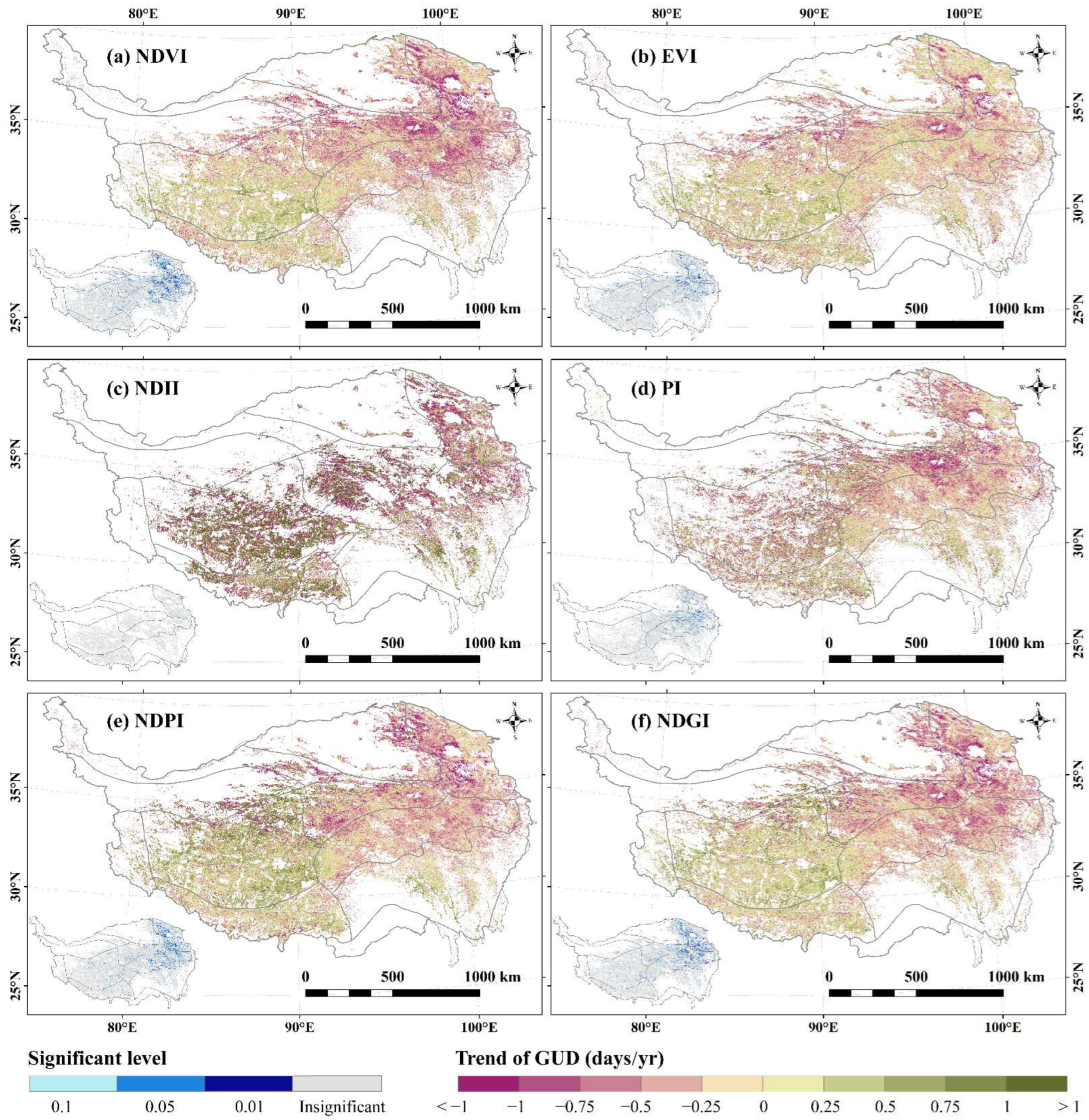
3.4.1. Trend Analysis

The inter-annual variation trend of vegetation GUD were analyzed at each pixel using Theil-Sen non-parametric regression [59,60]. All pairwise slopes of the time series data were calculated using this method, with the median slope representing the overall trend of change throughout the study period. Compared with traditional least-squares linear regressions, this approach does not require the independence and normality of the time series data, and is robust against outliers. The magnitude of the trend was measured using β, which is defined as follows:
β = m e d i a n ( x i x j i j ) ,     1 < j < i < n
where β is the slope of the trend, n represents the length of the time series, and x i and x j are the ith and jth data values in the time series, respectively. The significance of the trend was inspected using the Mann–Kendall test [61].

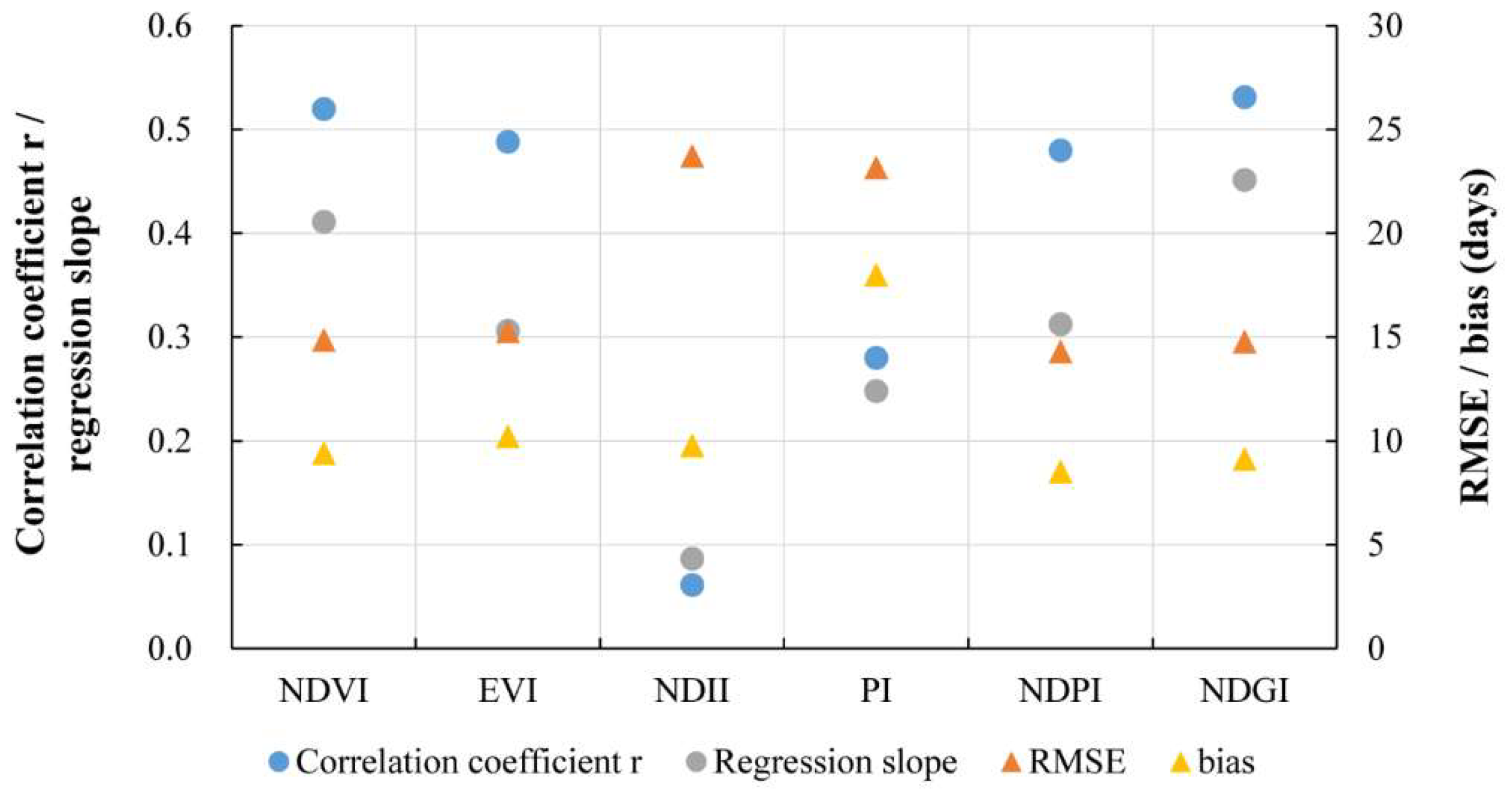
3.4.2. Accuracy Assessment

The accuracy of GUDs derived from different VIs and extraction methods was evaluated by comparison with the ground-observed GUD from 19 agrometeorological stations over the TP. The trends of satellite and ground-observed GUDs have been proven to be consistent over time and space, despite the differences in their differences [14]. Satellite GUDs within a 10 km × 10 km (21 pixels × 21 pixels) window centered on each station were used to calculate the mean value. This mean value and the ground-observed GUD at the station form one pair and 19 × 11 (station × year) pairs of GUDs was obtained for each VI (or each extraction method). All the GUD pairs during 2003–2013 were then analyzed for each VI (or each extraction method) using a simple linear regression model. Four indices, namely the Pearson’s correlation coefficient r, regression slope, root mean square error (RMSE), and bias, were used for accuracy assessment. We also explained the impact of preseason snow cover on GUDs extracted from different VIs by comparing the accuracy in pixel-years with and without preseason snow cover. A pixel-year was marked as affected by preseason snow cover if SCED occurred within two months prior to GUD [62]. To explain the differences between GUDs extracted though different methods, we further calculated and compared the threshold percentage of VI curve amplitude corresponding to ground-observed GUD and satellite-observed GUD for different vegetation types at agrometeorological stations.

4. Results

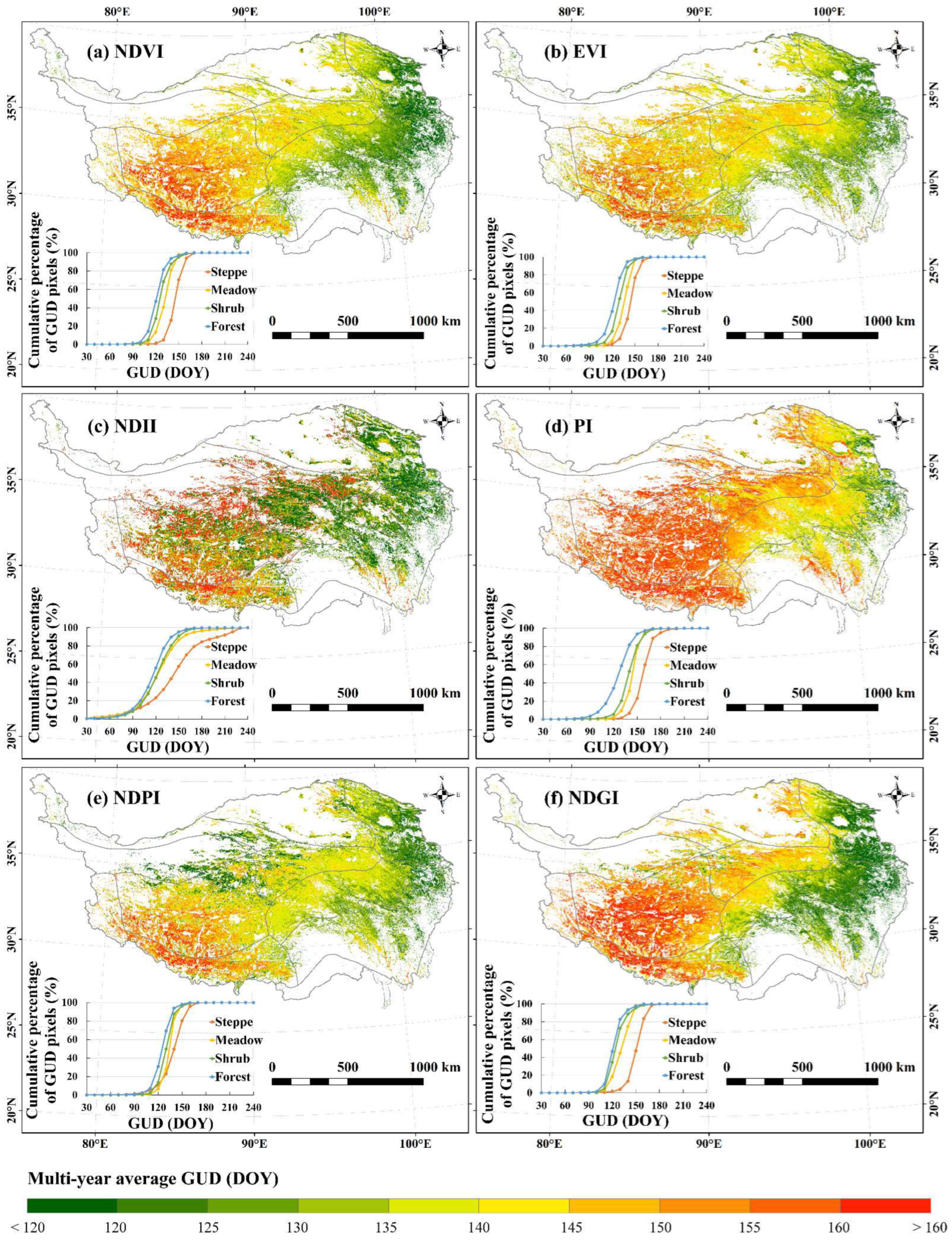
4.1. Spatiotemporal Variation of GUD

Figure 2a–f shows the spatial patterns of the GUDs derived from six VIs. Each subgraph shows the multi-year mean GUD of each pixel which is obtained by averaging all the GUDs at each pixel given by the four methods (βmax, CCRmax, G20, and RCmax) from 2003 to 2020. The cumulative percentage of GUD pixels for each vegetation type is displayed in the lower left of each subgraph. To facilitate discussion, GUDNDVI, GUDEVI, GUDNDII, GUDPI, GUDNDPI, and GUDNDGI represent hereafter GUD derived from NDVI, EVI, NDII, PI, NDPI, and NDGI, respectively. Generally, GUDs derived from different VIs mainly occurred from 120 to 160 DOY (May to 9 June), and showed a similar delay from east to west, with a great spatial heterogeneity over the whole plateau. Across all vegetation types, the GUD of forests occurred the earliest, followed by that of shrubs and meadows, and finally the alpine steppes. The earliest GUD (before 130 DOY, 10 May) mainly occurred in sub-humid regions (HIIAB1, HIB1, and HIIC1), and the latest GUD (after 150 DOY, 30 May) mainly occurred in semi-arid regions (HIC2 and HIIC2).
Specific spatial differences between the GUDs extracted from different VIs can be observed. GUDNDVI, GUDEVI, GUDNDPI, and GUDNDGI mainly occurred during the period of 120–150 DOY (May) (Figure 2a,b,e,f). These four showed consistently that forests mainly greened from 110 to 130 DOY (20 April to 10 May), shrubs from 110 to 140 DOY (20 April to 20 May), meadows from 120 to 150 DOY (May), and steppes from 130 to 160 DOY (10 May to 9 June). GUDNDII had a relatively longer time span, mostly ranging from 100 to 165 DOY (early April to middle June) in most regions (Figure 2c). The spatial transitions of GUDNDII are less obvious compared to the other GUDs since the steppe was the latest to fully green up—until nearly 230 DOY (mid-August). GUDPI occurred generally later in the entire plateau, mainly from 135 to 160 DOY (15 May to 9 June) (Figure 2d). The differences in GUDPI among the different vegetation types were larger.
Figure 3 shows the temporal variation trends of the GUDs from 2003 to 2020. The significance of the trend was marked in the lower left of each subgraph. Generally, the GUDs derived from different VIs were advanced in the eastern, but delayed in the western part of the plateau during the study period. This trend was significant mainly in the northeast part of TP. Nearly half of the study area had advanced GUD from 2003 to 2020. The average advancement determined from GUDNDVI, GUDEVI, GUDNDII, GUDPI, GUDNDPI, and GUDNDGI were −0.92, −0.7, −0.44, −0.90, −0.74, and −0.84 days/year (p < 0.01), respectively. The delayed GUD was mainly distributed in the southwest, but the trend of delay was almost less than 1 day/year, and was not significant. Among the different vegetation types, the meadows had the most significant trend of advancement, while the steppe’s variation trend was the mildest and was insignificant. The areas with the most advanced GUD were located in sub-humid and semi-arid regions (HIB1, HIC1, and HIIC1).

4.2. Performance of VIs in GUD Extraction

Different VIs and extraction methods lead to different GUD accuracies. The performances of the six VIs for capturing GUD were first evaluated through the comparison of correlation coefficient r, linear regression slope, RMSE, and bias between the ground-observed GUDs and satellite-observed GUDs between 2003 and 2013 (Figure 4). Each VI was combined using all four methods. The results showed that NDVI, EVI, NDPI, and NDGI can capture GUD with the r higher than 0.48, the regression slope greater than 0.30, the RMSE of approximately 15 days, and the bias of approximately 10 days. It is worth noting that the NDVI and EVI here have been preprocessed to remove snow influences. Among them, NDGI achieved the largest r (r = 0.53) and regression slope (slope = 0.45), indicating that the GUD extracted from NDGI had the best consistency with ground observations. However, NDII and PI showed a lower correlation and greater difference with ground observations than the other VIs.
Snow cover in early spring can affect GUD identification [21,62]. To understand the influence of preseason snow cover on the accuracy of GUD extracted from the six VIs, we further divided all site-years into categories of with and without preseason snow cover, and tested the correlation coefficient r, regression slope, RMSE, and bias between ground-observed GUD and satellite-observed GUDs under these two cases (Table 1). Here, satellite-observed GUDs were detected from six VIs using CCRmax. For the site-years without preseason snow cover, the comparison between ground-observed GUD and satellite-observed GUDs derived from six VIs showed significant positive correlations. NDGI had the best performance in the snow-free case, with the highest r value, lowest RMSE, and smallest bias (r = 0.60, p < 0.01, RMSE = 11.06 days, bias = −3.80 days). NDVI (r = 0.58, p < 0.01, RMSE = 14.03 days, bias = −8.70 days), NDPI (r = 0.57, p < 0.01, RMSE = 12.78 days, bias = −6.81 days) and EVI (r = 0.52, p < 0.01, RMSE = 13.96 days, bias = −8.30 days) also had relatively good correlation with ground-observed GUD. The GUDs extracted from NDII and PI were weakly correlated with the ground-observation GUD. For the preseason-snow-covered site-years, NDVI (r = 0.72, p < 0.01), NDGI (r = 0.71, p < 0.01), EVI (r = 0.63, p < 0.01), and NDPI (r = 0.57, p < 0.01) still performed well with a significant correlation with ground-observed GUD. Among them, NDGI had a lower RMSE and bias (RMSE = 10.69 days, bias = −4.05 days) than the other VIs. GUDs extracted from NDII were negatively correlated with and greatly deviated from ground observations, indicating that preseason snow cover caused a great disturbance to GUD extraction from NDII.
For almost all the VIs, the derived GUDs had stronger correlation with ground observation in preseason-snow-covered areas than in preseason-snow-free areas. Similar findings were also concluded in the study of Huang et al. [62]. The possible reason is that the sample number of site-years with preseason snow cover (sample number = 32) was much lower than that of sites without preseason snow cover (sample number = 168), thus resulting in the difference between the correlation results.

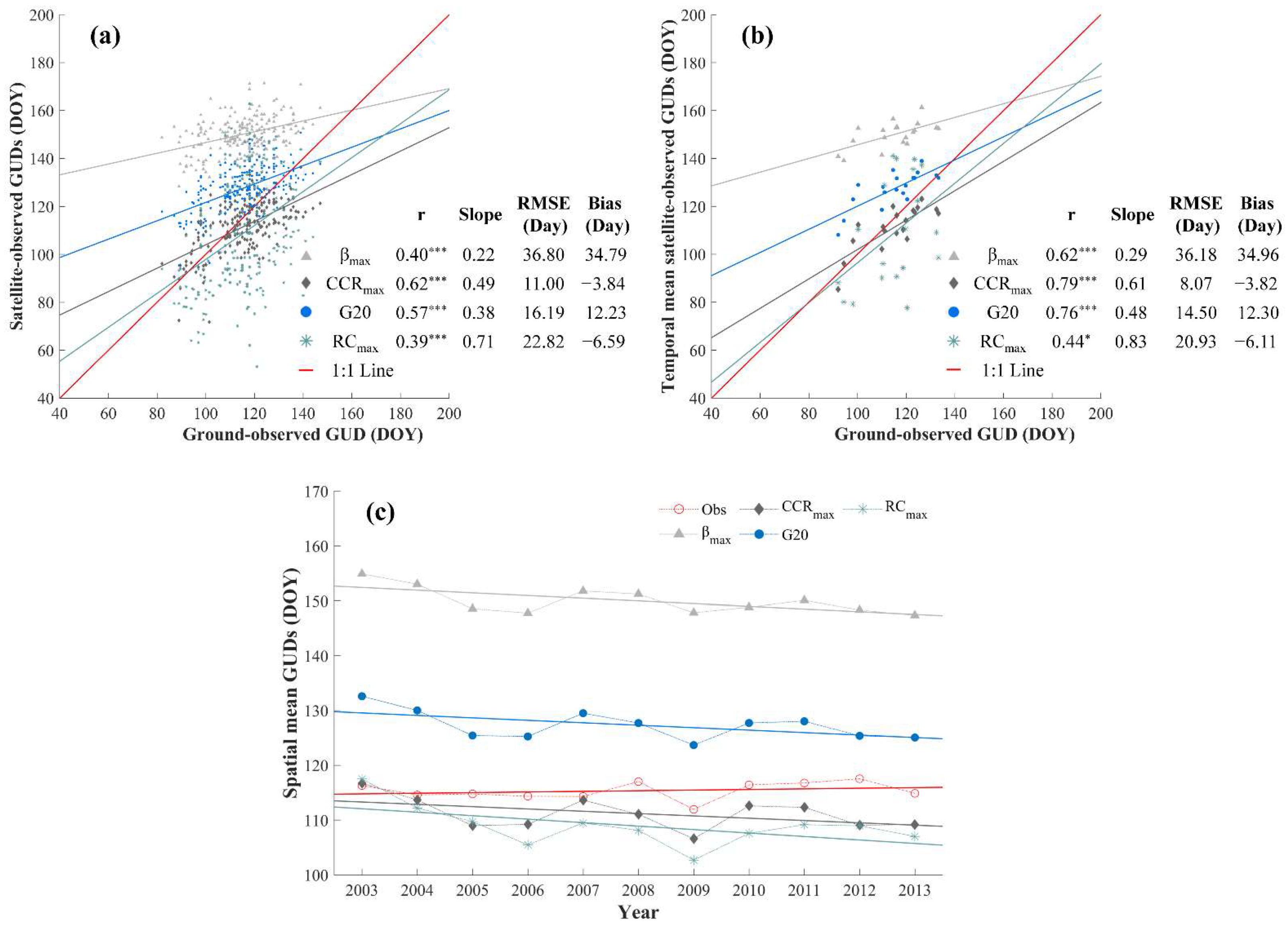
4.3. Performance of GUD Extraction Methods

The above results suggest that NDGI had the best performance and is suitable for GUD detection. Next, we focused on NDGI to evaluate the performance of the four GUD extraction methods (Figure 5). The comparison between ground-observed GUD and satellite-observed GUDs derived through the four methods showed significant correlations for all site-years (Figure 5a). CCRmax obtained the most accurate GUD with the highest r, lowest RMSE, and smallest bias (r = 0.62, p < 0.01, RMSE = 11 days, bias = −3.84 days). βmax had a relatively lower r, the highest RMSE, and the largest bias (r = 0.40, p < 0.01, RMSE = 36.80 days, bias = 34.79 days). When the comparison was conducted between the multi-year averaged satellite-based and ground-based GUDs (in total 19 GUD pairs for each extraction method), the linear correlations became stronger (Figure 5b), with CCRmax still having the strongest relationship (r = 0.79, p < 0.01, RMSE = 8.07 days, bias = −3.82 days) compared to the other methods (Figure 5b). We further compared the interannual variations and trends of the spatially averaged GUDs extracted using different methods (Figure 5c). The trend of GUD was 0.11 days/year (p > 0.1) for ground observation, and was −0.49 days/year (p < 0.05) for GUD detected by βmax, −0.42 days/year (p > 0.1) for GUD detected by CCRmax, −0.45 days/year (p < 0.1) for GUD detected by G20, −0.63 days/year (p < 0.1) for GUD detected by RCmax. Although not all the trends were significant, the GUD estimated through CCRmax was closest to the ground observation trend, while the other methods were different. In summary, CCRmax was the most accurate and suitable method for GUD extraction.

5. Discussion

5.1. Applicability of Snow-Free VIs on the TP

GUD derived from conventional VIs, such as NDVI and EVI, can be affected by snow cover. To eliminate the influence of snowmelt on VIs, previous studies replaced snow-polluted VI values with unpolluted VI values (e.g., [63,64]), which was the method we used to process NDVI and EVI in this study. By comparing the accuracy of GUDs extracted by the two VIs with and without snow calibration (Table 2), we found that snow calibration can significantly improve the r value (increased by 0.42 for NDVI, 0.43 for EVI) and regression slope (increased by 0.26 for NDVI, 0.25 for EVI), while significantly reducing RMSE (reduced by 9.13 days for NDVI, 9.39 days for EVI) and bias (reduced by 1.93 days for NDVI, 1.84 days for EVI).
Snow-free VIs have been proposed to account for and minimize the influence of snow cover on GUD monitoring, such as NDII, PI, NDPI, and NDGI. However, they still have some drawbacks in GUD detection. NDII is sensitive to moisture because of the incorporation of SWIR spectral band [20], leading to higher values over snow than for vegetation [21]. Therefore, NDII can increase during vegetation growth and decrease with snow melt [22], both of which happen in the spring season, thus resulting in overestimation of GUD [20]. The PI was designed to reflect a more realistic status of vegetation growth by singling out the impact of wetness from greenness [21]. For ice, snow, and water that result in NDVI < 0, PI is assigned 0; for soil and non-photosynthetic vegetation components that result in NDII < 0, PI is assigned 0 [21]. However, sparse vegetation cannot be recognized by PI [24], usually leading to the overestimated GUD.
Our results indicate that NDPI and NDGI can capture the TP’s surface GUD, giving better results than the NDVI and EVI after snow calibration (Figure 4). In particular, the NDGI achieved the highest accuracy. The GUD estimated by NDPI showed a greater negative bias than that estimated by NDGI, mainly in the southwest TP with arid alpine steppe as the main vegetation type. Similar results were also found in studies at grassland flux tower sites in the middle and high latitudes [23], and NDPI has been proved to have greater uncertainty in GUD extraction than NDGI in grasslands in Kazakhstan, Mongolia, and North Asia [25]. The probable reason is that NDGI accounts for dry grass—whose reflectance varies almost linearly from green to NIR—and the rationale behind NDGI gives dry grass a value of approximately zero [23]. NDPI is based on the assumption that the reflectance of background components (soil and snow) varies monotonously from red to NIR to SWIR bands and is designed to be close to zero on the background component [24]. However, the spectral characteristics of dry grass showed nearly equal reflectance in the NIR and SWIR bands. Therefore, the NDPI value of dry grass will be higher than those of other background components, which may be mistaken as vegetation growth and result in an underestimation of GUD. Nevertheless, it has also been found that NDPI performs better than NDGI in the absence of dry grass due to its better ability to suppress variations in soil background [24], indicating the unique value of NDPI for deciduous ecosystem. These results inspired us to select the most suitable VI for GUD extraction according to the vegetation types and environmental conditions of the study area. In addition, these two snow-free VIs can be easily and expediently calculated from multiband surface reflectance data, giving it an advantage over the practice of eliminating snow cover from traditional VIs with the help of auxiliary data.

5.2. Impact of Extraction Methods on GUD Accuracy

In this study, although the GUDs extracted by the four methods were significantly correlated with the ground observation, there were obvious differences in the accuracy of GUDs determined by different extraction methods (Figure 5). Figure 6 shows the threshold percentage of NDGI curve amplitude corresponding to ground-observed GUD and satellite-observed GUD for the four vegetation types. We found that the NDGI threshold percentage of ground-observed GUD ranged from 8% to 16%, and varied with vegetation type (Figure 6). This implies that a single relative threshold cannot capture a GUD with 100% accuracy. In addition, the NDGI threshold percentage varies with different GUD extraction methods; thus, different GUD extraction methods reflect different stages of plant growth [41]. For example, the NDGI threshold percentages for CCRmax and βmax were approximately 9.18% and 50%, respectively (Figure 6), which was also found in a previous study [65]. Therefore, CCRmax is more likely to detect GUD in the early stages of vegetation growth, whereas βmax favors exuberant photosynthesis and fast plant growth.
CCRmax showed higher GUD extraction accuracy than the other methods (Figure 5), which is consistent with previous studies on winter wheat in the Huanghuai region [26] and for grassland on the TP [66]. There are two probable reasons for CCRmax’s superiority. First, the NDGI threshold percentage of the GUD extracted by CCRmax was closest to that of ground observation (Figure 6). Second, CCRmax is less affected by fluctuations in the initial background VI value, which is more susceptible to noise [66].
βmax and G20 overestimate the GUD, and βmax has a larger positive deviation and lower correlation with ground observations than G20 in GUD extraction (Figure 5). This result is reasonable, since the βmax is mostly equivalent to the 50% relative threshold method (G50). Many studies have found that G20 gained a GUD that is closer to and more correlated with ground observations than G50 [67]. This is probably because GUD at the species scale cannot be reflected by a 50% relative threshold [68].
RCmax acts similarly by setting a fixed NDGI threshold for each pixel, marking the multi-year averaged NDGI with the fastest growth rate [33]. Therefore, RCmax is more sensitive to the shape and interannual variation in the VI curve. The corresponding NDGI threshold percentages of RCmax differ for different vegetation types, mainly 26–52% for steppe and 2–10% for meadows, shrubs, and forests (Figure 6). Therefore, the accuracy of GUD extracted by RCmax may have greater spatial heterogeneity. Therefore, CCRmax is recommended for GUD extraction in combination with NDGI on the TP, and the uncertainty of GUD extraction using different methods in different study areas still deserves attention.

6. Conclusions

This study extracted satellite-based GUDs on the TP from six MODIS-derived VIs (NDVI, EVI, NDII, PI, NDPI, and NDGI) by applying four different extraction methods (βmax, CCRmax, G20, and RCmax). We evaluated the spatial distribution and temporal variation trends of GUD on the TP. We then assessed the accuracy of satellite-based GUDs by comparison with ground-observed GUD from 19 agrometeorological stations, using Pearson’s correlation, linear regression, RMSE, and bias.
The results show that the GUD on the TP mainly occurred from 120 to 160 DOY (May to 9 June), and it was early in the eastern and late in the western part of the plateau. GUD occurred earliest in forests for all vegetation types, followed by shrubs and meadows, and alpine steppes were the latest. During the study period, the GUD advanced in the eastern region but was delayed in the western part of the plateau. The GUD of meadows in the northeastern TP exhibited and the most significant advancement. The GUD variation trend in the western and southeastern plateau is mild and insignificant.
The accuracy assessment of the GUD showed that different VIs and extraction methods produced different levels of uncertainties in GUD detection. NDGI, NDPI, and snow-calibrated NDVI and EVI can capture GUD and maintain favorable accuracy for areas with preseason snow cover, whereas NDII and PI hardly captured GUD. NDGI was superior to the other VIs in GUD extraction, with the highest overall accuracy. We also found that the GUD extracted by CCRmax had the best consistency with ground observations. In addition, our experiment proved that snow calibration could significantly improve the accuracy of GUD extracted from NDVI and EVI. In contrast, the snow-free VIs, NDGI and NDPI, were able to achieve similar or even better accuracies than NDVI and EVI after snow calibration. Our research substantiates the applicability of snow-free VIs, particularly NDGI, for GUD detection on the TP. These results provide a significant perspective for analyzing vegetation dynamics on the TP.

Author Contributions

Conceptualization, J.C. and Y.H.; Methodology, J.X. (Jingyi Xu), Y.T. and K.B.; Validation, J.X. (Jingyi Xu), Y.T. and J.X. (Jiahui Xu); Formal Analysis, J.X. (Jingyi Xu), J.C., B.Y., J.W. and Y.H.; Writing—Original Draft Preparation, J.X. (Jingyi Xu); Writing—Review and Editing, S.S. and Y.H.; Visualization, J.X. (Jingyi Xu) and Y.T.; Supervision, Y.H.; Funding Acquisition, Y.H. All authors have read and agreed to the published version of the manuscript.

Funding

This work was supported by the National Natural Science Foundation of China (Grant No. 42071306).

Data Availability Statement

The data that support the findings of this study are available from the website given in the manuscript.

Acknowledgments

We would like to thank National Meteorological Information Centre of China Meteorological Administration for providing the phenology data over the Tibetan Plateau.

Conflicts of Interest

The authors declare no conflict of interest.

Appendix A

Table A1. Eco-geographical regions of the TP [45].
Temperature ZoneHumidity RegionEco-Geographical Region
HI Plateau sub-cold zoneB Sub-humid regionHIB1 Golog-Naqu hummocky plateau shrub-meadow region
C Semi-arid regionHIC1 South Qinghai plateau wide valley meadow-steppe region
HIC2 Qiangtang plateau lake basin steppe region
D Arid regionHID1 Kunlun high mountain plateau desert region
HII Plateau temperate zoneA/B Humid/sub-humid regionHIIA/B1 West Sichuan and east Tibet high mountain and deep valley coniferous forest region
C Semi-arid regionHIIC1 Qilian Mountains of east Qinghai coniferous forest-steppe region
HIIC2 South Tibet Mountain shrub-steppe region
D Arid regionHIID1 Qaidam basin desert region
HIID2 North wing of Kunlun Mountain desert region
HIID3 Ngari Mountain desert region
V Middle subtropical zoneA Humid regionVA6 South wing of east Himalaya Mountain seasonal rainforest evergreen broad-leaved forest region

References

  1. Qiu, J. The third pole. Nature 2008, 454, 393–396. [Google Scholar] [CrossRef] [PubMed] [Green Version]
  2. Dong, M.; Jiang, Y.; Zheng, C.; Zhang, D. Trends in the thermal growing season throughout the Tibetan Plateau during 1960–2009. Agric. For. Meteorol. 2012, 166–167, 201–206. [Google Scholar] [CrossRef]
  3. Zhang, X.; Friedl, M.A.; Schaaf, C.B.; Strahler, A.H.; Hodges, J.C.F.; Gao, F.; Reed, B.C.; Huete, A. Monitoring vegetation phenology using MODIS. Remote Sens. Environ. 2003, 84, 471–475. [Google Scholar] [CrossRef]
  4. Keenan, T.F.; Gray, J.; Friedl, M.A.; Toomey, M.; Bohrer, G.; Hollinger, D.Y.; Munger, J.W.; O’Keefe, J.; Schmid, H.P.; SueWing, I.; et al. Net carbon uptake has increased through warming-induced changes in temperate forest phenology. Nat. Clim. Chang. 2014, 4, 598–604. [Google Scholar] [CrossRef]
  5. Zha, T.S.; Barr, A.G.; van der Kamp, G.; Black, T.A.; McCaughey, J.H.; Flanagan, L.B. Interannual variation of evapotranspiration from forest and grassland ecosystems in Western Canada in relation to drought. Agric. For. Meteorol. 2010, 150, 1476–1484. [Google Scholar] [CrossRef]
  6. Richardson, A.D.; Keenan, T.F.; Migliavacca, M.; Ryu, Y.; Sonnentag, O.; Toomey, M. Climate change, phenology, and phenological control of vegetation feedbacks to the climate system. Agric. For. Meteorol. 2013, 169, 156–173. [Google Scholar] [CrossRef]
  7. Pettorelli, N.; Vik, J.O.; Mysterud, A.; Gaillard, J.-M.; Tucker, C.J.; Stenseth, N.C. Using the satellite-derived NDVI to assess ecological responses to environmental change. Trends Ecol. Evol. 2005, 20, 503–510. [Google Scholar] [CrossRef]
  8. Wolkovich, E.M.; Cook, B.I.; Allen, J.M.; Crimmins, T.M.; Betancourt, J.L.; Travers, S.E.; Pau, S.; Regetz, J.; Davies, T.J.; Kraft, N.J.; et al. Warming experiments underpredict plant phenological responses to climate change. Nature 2012, 485, 494–497. [Google Scholar] [CrossRef]
  9. Wingate, L.; Ogee, J.; Cremonese, E.; Filippa, G.; Mizunuma, T.; Migliavacca, M.; Moisy, C.; Wilkinson, M.; Moureaux, C.; Wohlfahrt, G.; et al. Interpreting canopy development and physiology using a European phenology camera network at flux sites. Biogeosciences 2015, 12, 5995–6015. [Google Scholar] [CrossRef] [Green Version]
  10. Berra, E.F.; Gaulton, R.; Barr, S. Assessing spring phenology of a temperate woodland: A multiscale comparison of ground, unmanned aerial vehicle and Landsat satellite observations. Remote Sens. Environ. 2019, 223, 229–242. [Google Scholar] [CrossRef]
  11. Wu, C.Y.; Chen, J.M.; Black, T.A.; Price, D.T.; Kurz, W.A.; Desai, A.R.; Gonsamo, A.; Jassal, R.S.; Gough, C.M.; Bohrer, G.; et al. Interannual variability of net ecosystem productivity in forests is explained by carbon flux phenology in autumn. Global Ecol. Biogeogr. 2013, 22, 994–1006. [Google Scholar] [CrossRef]
  12. Richardson, A.D.; Hufkens, K.; Milliman, T.; Aubrecht, D.M.; Chen, M.; Gray, J.M.; Johnston, M.R.; Keenan, T.F.; Klosterman, S.T.; Kosmala, M.; et al. Tracking vegetation phenology across diverse North American biomes using PhenoCam imagery. Sci. Data 2018, 5, 24. [Google Scholar] [CrossRef] [PubMed]
  13. Jeong, S.J.; Schimel, D.; Frankenberg, C.; Drewry, D.T.; Fisher, J.B.; Verma, M.; Berry, J.A.; Lee, J.E.; Joiner, J. Application of satellite solar-induced chlorophyll fluorescence to understanding large-scale variations in vegetation phenology and function over northern high latitude forests. Remote Sens. Environ. 2017, 190, 178–187. [Google Scholar] [CrossRef]
  14. Guo, L.; An, N.; Wang, K. Reconciling the discrepancy in ground- and satellite-observed trends in the spring phenology of winter wheat in China from 1993 to 2008. J. Geophys. Res. Atmos. 2016, 121, 1027–1042. [Google Scholar] [CrossRef] [Green Version]
  15. Rouse, J.W.; Haas, R.H.; Schell, J.A.; Deering, D.W. Monitoring Vegetation Systems in the Great Plains with ERTS; Freden, S.C., Mercanti, E.P., Becker, M., Eds.; NASA: Washington, DC, USA, 1973; pp. 309–317.
  16. Liu, H.Q.; Huete, A. A feedback based modification of the NDVI to minimize canopy background and atmospheric noise. IEEE Trans. Geosci. Remote Sens. 1995, 33, 457–465. [Google Scholar] [CrossRef]
  17. Huete, A.; Didan, K.; Miura, T.; Rodriguez, E.P.; Gao, X.; Ferreira, L.G. Overview of the radiometric and biophysical performance of the MODIS vegetation indices. Remote Sens. Environ. 2002, 83, 195–213. [Google Scholar] [CrossRef]
  18. Matsushita, B.; Yang, W.; Chen, J.; Onda, Y.; Qiu, G.Y. Sensitivity of the Enhanced Vegetation Index (EVI) and Normalized Difference Vegetation Index (NDVI) to topographic effects: A case study in high-density cypress forest. Sensors 2007, 7, 2636–2651. [Google Scholar] [CrossRef] [Green Version]
  19. Shen, M.; Sun, Z.; Wang, S.; Zhang, G.; Kong, W.; Chen, A.; Piao, S. No evidence of continuously advanced green-up dates in the Tibetan Plateau over the last decade. Proc. Natl. Acad. Sci. USA 2013, 110, E2329. [Google Scholar] [CrossRef] [Green Version]
  20. Delbart, N.; Kergoat, L.; Le Toan, T.; Lhermitte, J.; Picard, G. Determination of phenological dates in boreal regions using normalized difference water index. Remote Sens. Environ. 2005, 97, 26–38. [Google Scholar] [CrossRef] [Green Version]
  21. Gonsamo, A.; Chen, J.M.; Price, D.T.; Kurz, W.A.; Wu, C. Land surface phenology from optical satellite measurement and CO2 eddy covariance technique. J. Geophys. Res. Biogeosci. 2012, 117, 18. [Google Scholar] [CrossRef]
  22. Peckham, S.D.; Ahl, D.E.; Serbin, S.P.; Gower, S.T. Fire-induced changes in green-up and leaf maturity of the Canadian boreal forest. Remote Sens. Environ. 2008, 112, 3594–3603. [Google Scholar] [CrossRef]
  23. Yang, W.; Kobayashi, H.; Wang, C.; Shen, M.; Chen, J.; Matsushita, B.; Tang, Y.; Kim, Y.; Bret-Harte, M.S.; Zona, D.; et al. A semi-analytical snow-free vegetation index for improving estimation of plant phenology in tundra and grassland ecosystems. Remote Sens. Environ. 2019, 228, 31–44. [Google Scholar] [CrossRef]
  24. Wang, C.; Chen, J.; Wu, J.; Tang, Y.; Shi, P.; Black, T.A.; Zhu, K. A snow-free vegetation index for improved monitoring of vegetation spring green-up date in deciduous ecosystems. Remote Sens. Environ. 2017, 196, 1–12. [Google Scholar] [CrossRef]
  25. Cao, R.Y.; Feng, Y.; Liu, X.L.; Shen, M.G.; Zhou, J. Uncertainty of vegetation green-up date estimated from vegetation indices due to snowmelt at northern middle and high latitudes. Remote Sens. 2020, 12, 190. [Google Scholar] [CrossRef] [Green Version]
  26. Gan, L.; Cao, X.; Chen, X.; Dong, Q.; Cui, X.; Chen, J. Comparison of MODIS-based vegetation indices and methods for winter wheat green-up date detection in Huanghuai region of China. Agric. For. Meteorol. 2020, 288–289, 108019. [Google Scholar] [CrossRef]
  27. Zeng, L.L.; Wardlow, B.D.; Xiang, D.X.; Hu, S.; Li, D.R. A review of vegetation phenological metrics extraction using time-series, multispectral satellite data. Remote Sens. Environ. 2020, 237, 20. [Google Scholar] [CrossRef]
  28. Myneni, R.B.; Keeling, C.D.; Tucker, C.J.; Asrar, G.; Nemani, R.R. Increased plant growth in the northern high latitudes from 1981 to 1991. Nature 1997, 386, 698–702. [Google Scholar] [CrossRef]
  29. White, M.A.; Thornton, P.E.; Running, S.W. A continental phenology model for monitoring vegetation responses to interannual climatic variability. Glob. Biogeochem. Cycles 1997, 11, 217–234. [Google Scholar] [CrossRef]
  30. Yu, H.; Luedeling, E.; Xu, J. Winter and spring warming result in delayed spring phenology on the Tibetan Plateau. Proc. Natl. Acad. Sci. USA 2010, 107, 22151–22156. [Google Scholar] [CrossRef] [Green Version]
  31. Tan, B.; Morisette, J.T.; Wolfe, R.E.; Gao, F.; Ederer, G.A.; Nightingale, J.; Pedelty, J.A. An enhanced TIMESAT algorithm for estimating vegetation phenology metrics from MODIS data. IEEE J. Sel. Top. Appl. Earth Obs. Remote Sens. 2011, 4, 361–371. [Google Scholar] [CrossRef]
  32. Lu, L.L.; Wang, C.Z.; Guo, H.D.; Li, Q.T. Detecting winter wheat phenology with SPOT-VEGETATION data in the North China Plain. Geocarto Int. 2014, 29, 244–255. [Google Scholar] [CrossRef]
  33. Piao, S.L.; Fang, J.Y.; Zhou, L.M.; Ciais, P.; Zhu, B. Variations in satellite-derived phenology in China’s temperate vegetation. Global Change Biol. 2006, 12, 672–685. [Google Scholar] [CrossRef]
  34. Zheng, Z.T.; Zhu, W.Q. Uncertainty of remote sensing data in monitoring vegetation phenology: A comparison of MODIS C5 and C6 vegetation index products on the Tibetan Plateau. Remote Sens. 2017, 9, 1288. [Google Scholar] [CrossRef] [Green Version]
  35. Keatley, M.R.; Hudson, I.L. Phenological Research Methods for Environmental and Climate Change Analysis Introduction and Overview; Hudson, I.L., Keatley, M.R., Eds.; Springer: New York, NY, USA, 2010; pp. 1–22. [Google Scholar] [CrossRef]
  36. de Beurs, K.M.; Henebry, G.M. Spatio-Temporal Statistical Methods for Modelling Land Surface Phenology; Hudson, I.L., Keatley, M.R., Eds.; Springer: New York, NY, USA, 2010; pp. 177–208. [Google Scholar] [CrossRef]
  37. Sakamoto, T.; Wardlow, B.D.; Gitelson, A.A.; Verma, S.B.; Suyker, A.E.; Arkebauer, T.J. A Two-Step Filtering approach for detecting maize and soybean phenology with time-series MODIS data. Remote Sens. Environ. 2010, 114, 2146–2159. [Google Scholar] [CrossRef]
  38. Pan, Z.K.; Huang, J.F.; Zhou, Q.B.; Wang, L.M.; Cheng, Y.X.; Zhang, H.K.; Blackburn, G.A.; Yan, J.; Liu, J.H. Mapping crop phenology using NDVI time-series derived from HJ-1 A/B data. Int. J. Appl. Earth Obs. Geoinf. 2015, 34, 188–197. [Google Scholar] [CrossRef] [Green Version]
  39. Xu, X.M.; Conrad, C.; Doktor, D. Optimising phenological metrics extraction for different crop types in Germany using the Moderate Resolution Imaging Spectrometer (MODIS). Remote Sens. 2017, 9, 254. [Google Scholar] [CrossRef] [Green Version]
  40. Zeng, L.L.; Wardlow, B.D.; Wang, R.; Shan, J.; Tadesse, T.; Hayes, M.J.; Li, D.R. A hybrid approach for detecting corn and soybean phenology with time-series MODIS data. Remote Sens. Environ. 2016, 181, 237–250. [Google Scholar] [CrossRef]
  41. White, M.A.; de Beurs, K.M.; Didan, K.; Inouye, D.W.; Richardson, A.D.; Jensen, O.P.; O’Keefe, J.; Zhang, G.; Nemani, R.R.; van Leeuwen, W.J.D.; et al. Intercomparison, interpretation, and assessment of spring phenology in North America estimated from remote sensing for 1982–2006. Glob. Chang. Biol. 2009, 15, 2335–2359. [Google Scholar] [CrossRef]
  42. Wang, H.J.; Dai, J.H.; Ge, Q.S. Comparison of satellite and ground-based phenology in China’s temperate monsoon area. Adv. Meteorol. 2014, 2014, 10. [Google Scholar] [CrossRef]
  43. Zhang, X.X.; Cui, Y.P.; Qin, Y.C.; Xia, H.M.; Lu, H.L.; Liu, S.J.; Li, N.; Fu, Y.M. Evaluating the accuracy of and evaluating the potential errors in extracting vegetation phenology through remote sensing in China. Int. J. Remote Sens. 2020, 41, 3592–3613. [Google Scholar] [CrossRef]
  44. Peng, J.; Liu, Z.; Liu, Y.; Wu, J.; Han, Y. Trend analysis of vegetation dynamics in Qinghai–Tibet Plateau using Hurst Exponent. Ecol. Indic. 2012, 14, 28–39. [Google Scholar] [CrossRef]
  45. Wu, S.; Yang, Q.; Du, Z. Delineation of eco-geographic regional system of China. J. Geog. Sci. 2003, 13, 309–315. [Google Scholar] [CrossRef]
  46. Pu, Z.; Xu, L.; Salomonson, V.V. MODIS/Terra observed seasonal variations of snow cover over the Tibetan Plateau. Geophys. Res. Lett. 2007, 34, 6. [Google Scholar] [CrossRef] [Green Version]
  47. Vermote, E.F.; Roger, J.C.; Ray, J.P. MODIS Surface Reflectance Collection 6 User’s Guide. Available online: https://modis-land.gsfc.nasa.gov/pdf/MOD09_UserGuide_v1.4.pdf (accessed on 8 December 2020).
  48. Holben, B.N. Characteristics of maximum-value composite images from temporal AVHRR data. Int. J. Remote Sens. 1986, 7, 1417–1434. [Google Scholar] [CrossRef]
  49. Savitzky, A.; Golay, M.J.E. Smoothing and differentiation of data by simplified least squares procedures. Anal. Chem. 1964, 36, 1627–1639. [Google Scholar] [CrossRef]
  50. Chen, J.; Jönsson, P.; Tamura, M.; Gu, Z.; Matsushita, B.; Eklundh, L. A simple method for reconstructing a high-quality NDVI time-series data set based on the Savitzky–Golay filter. Remote Sens. Environ. 2004, 91, 332–344. [Google Scholar] [CrossRef]
  51. Shen, M.G.; Zhang, G.X.; Cong, N.; Wang, S.P.; Kong, W.D.; Piao, S.L. Increasing altitudinal gradient of spring vegetation phenology during the last decade on the Qinghai-Tibetan Plateau. Agric. For. Meteorol. 2014, 189, 71–80. [Google Scholar] [CrossRef]
  52. Zhang, X.; Tarpley, D.; Sullivan, J.T. Diverse responses of vegetation phenology to a warming climate. Geophys. Res. Lett. 2007, 34, 5. [Google Scholar] [CrossRef]
  53. Huang, Y.; Liu, H.X.; Yu, B.L.; Wu, J.P.; Kang, E.L.; Xu, M.; Wang, S.J.; Klein, A.; Chen, Y.N. Improving MODIS snow products with a HMRF-based spatio-temporal modeling technique in the Upper Rio Grande Basin. Remote Sens. Environ. 2018, 204, 568–582. [Google Scholar] [CrossRef]
  54. Huang, Y.; Xu, J.; Xu, J.; Zhao, Y.; Yu, B.; Liu, H.; Wang, S.; Xu, W.; Wu, J.; Zheng, Z. HMRFS-TP: Long-term daily gap-free snow cover products over the Tibetan Plateau from 2002 to 2021 based on Hidden Markov Random Field model. Earth Syst. Sci. Data Discuss. 2022; in review. [Google Scholar] [CrossRef]
  55. Hardisky, M.A.; Klemas, V.; Smart, R.M. The influence of soil salinity, growth form, and leaf moisture on the spectral radiance of Spartina alterniflora canopies. Photogramm. Eng. Remote Sens. 1983, 49, 77–83. [Google Scholar]
  56. Helman, D. Land surface phenology: What do we really ‘see’ from space? Sci. Total Environ. 2018, 618, 665–673. [Google Scholar] [CrossRef] [PubMed]
  57. Chen, X.; Long, D.; Hong, Y.; Hao, X.; Hou, A. Climatology of snow phenology over the Tibetan plateau for the period 2001–2014 using multisource data. Int. J. Climatol. 2018, 38, 2718–2729. [Google Scholar] [CrossRef]
  58. Guo, H.; Wang, X.Y.; Guo, Z.C.; Chen, S.Y. Assessing snow phenology and its environmental driving factors in Northeast China. Remote Sens. 2022, 14, 262. [Google Scholar] [CrossRef]
  59. Theil, H. A rank-invariant method of linear and polynomial regression analysis. In Henri Theil’s Contributions to Economics and Econometrics: Econometric Theory and Methodology; Raj, B., Koerts, J., Eds.; Springer: Dordrecht, The Netherlands, 1992; pp. 345–381. [Google Scholar] [CrossRef]
  60. Sen, P.K. Estimates of the regression coefficient based on Kendall’s tau. J. Am. Stat. Assoc. 1968, 63, 1379–1389. [Google Scholar] [CrossRef]
  61. Kendall, M.G. A new measure of rank correlation. Biometrika 1938, 30, 81–93. [Google Scholar] [CrossRef]
  62. Huang, K.; Zhang, Y.; Tagesson, T.; Brandt, M.; Wang, L.; Chen, N.; Zu, J.; Jin, H.; Cai, Z.; Tong, X.; et al. The confounding effect of snow cover on assessing spring phenology from space: A new look at trends on the Tibetan Plateau. Sci. Total Environ. 2021, 756, 144011. [Google Scholar] [CrossRef]
  63. Beck, P.S.A.; Atzberger, C.; Høgda, K.A.; Johansen, B.; Skidmore, A.K. Improved monitoring of vegetation dynamics at very high latitudes: A new method using MODIS NDVI. Remote Sens. Environ. 2006, 100, 321–334. [Google Scholar] [CrossRef]
  64. Cao, R.; Chen, J.; Shen, M.; Tang, Y. An improved logistic method for detecting spring vegetation phenology in grasslands from MODIS EVI time-series data. Agric. For. Meteorol. 2015, 200, 9–20. [Google Scholar] [CrossRef]
  65. Shang, R.; Liu, R.; Xu, M.; Liu, Y.; Zuo, L.; Ge, Q. The relationship between threshold-based and inflexion-based approaches for extraction of land surface phenology. Remote Sens. Environ. 2017, 199, 167–170. [Google Scholar] [CrossRef]
  66. Li, N.; Zhan, P.; Pan, Y.Z.; Zhu, X.F.; Li, M.Y.; Zhang, D.J. Comparison of remote sensing time-series smoothing methods for grassland spring phenology extraction on the Qinghai-Tibetan Plateau. Remote Sens. 2020, 12, 3383. [Google Scholar] [CrossRef]
  67. Delbart, N.; Le Toan, T.; Kergoat, L.; Fedotova, V. Remote sensing of spring phenology in boreal regions: A free of snow-effect method using NOAA-AVHRR and SPOT-VGT data (1982–2004). Remote Sens. Environ. 2006, 101, 52–62. [Google Scholar] [CrossRef]
  68. Hamunyela, E.; Verbesselt, J.; Roerink, G.; Herold, M. Trends in spring phenology of Western European deciduous forests. Remote Sens. 2013, 5, 6159–6179. [Google Scholar] [CrossRef] [Green Version]
Figure 1. Spatial distributions of the land cover types and eco-geographical regions of the study area.
Remotesensing 14 03160 g001
Figure 2. The spatial variation in the multi-year mean GUD during 2003–2020 derived from each of the six VIs (NDVI, EVI, NDII, PI, NDPI and NDGI) averaged over the four methods (βmax, CCRmax, G20 and RCmax). The line chart in the lower left of each subgraph displays the cumulative percentage of GUD pixels for each vegetation type.
Remotesensing 14 03160 g002
Figure 3. Inter-annual trend of GUD derived from each of the six VIs (NDVI, EVI, NDII, PI, NDPI and NDGI) averaged over the four methods (βmax, CCRmax, G20 and RCmax) during 2003–2020. The map in the lower left of each subgraph shows the significance of trend at the 0.01, 0.05 and 0.1 levels.
Remotesensing 14 03160 g003
Figure 4. Correlation coefficient r, regression slope, RMSE, and bias between ground-observed GUD and satellite-observed GUDs detected from six VIs, each of which combined with four extraction methods.
Remotesensing 14 03160 g004
Figure 5. Performance comparison of GUD derived from NDGI through four methods (βmax, CCRmax, G20, RCmax). (a) Scatterplots and linear regression models of ground-observed GUD and satellite-observed GUDs extracted by the four methods for all site-years; (b) Scatterplots and linear regression models of the temporal-averaged GUDs for all sites. The symbols * and *** are significant at levels of 0.1 and 0.01, respectively. (c) Inter-annual variations and trends of spatial-averaged GUDs for all years. DOY, day of the year.
Remotesensing 14 03160 g005
Figure 6. The threshold percentage of NDGI curve amplitude of GUDs extracted with the four methods in different vegetation types at the agrometeorological stations.
Remotesensing 14 03160 g006
Table 1. Comparison between ground-observed GUD and satellite-observed GUDs detected from six VIs by CCRmax for site-years with and without preseason snow cover.
VIWithout Preseason Snow CoverWith Preseason Snow Cover
rSlopeRMSE
(Day)
Bias
(Day)
rSlopeRMSE
(Day)
Bias
(Day)
NDVI0.58 ***0.5314.03−8.700.72 ***0.4614.46−10.72
EVI0.52 ***0.4013.96−8.300.63 ***0.4212.48−6.25
NDII0.28 ***0.3924.02−15.33−0.34 *−0.9050.23−24.25
PI0.29 ***0.3016.907.800.38 **0.2715.877.95
NDPI0.57 ***0.4812.78−6.810.57 ***0.3512.38−4.66
NDGI0.60 ***0.4911.06−3.800.71 ***0.4410.69−4.05
The symbols *, **, and *** are significant at levels of 0.1, 0.05, and 0.01, respectively.
Table 2. Comparison between ground-observed GUD and GUDs extracted by CCRmax from two conventional VIs (NDVI and EVI) with and without snow calibration.
VIWhether to Calibrate SnowrSlopeRMSE (Day)Bias (Day)
NDVIuncalibrated0.18 **0.2723.23−10.95
snow-calibrated0.60 ***0.5314.10−9.02
EVIuncalibrated0.110.1623.12−9.81
snow-calibrated0.54 ***0.4113.73−7.97
The symbols ** and *** are significant at levels of 0.05 and 0.01, respectively.
Publisher’s Note: MDPI stays neutral with regard to jurisdictional claims in published maps and institutional affiliations.

