A Spherical “Earth–Ionosphere” Model for Deep Resource Exploration Using Artificial ELF-EM Field

Abstract

Fully coupled lithosphere, atmosphere, and ionosphere theory has demonstrated that extremely low-frequency electromagnetic (ELF-EM) fields present a broad application prospect in deep resource exploration, but previous studies have ignored the contribution of the Earth’s curvature. This study extends the theory of ELF-EM over a stratified Earth to the case where the Earth’s curvature must be taken into account, and presents an analytical solution of the ELF-EM field excited by a grounded horizontal antenna in a spherical Earth–ionosphere model, whose theoretical approach and solution method are notably different from the flat Earth–ionosphere model. Additionally, the Earth is treated as a concentric-layered sphere rather than an ideal homogeneous sphere. We aim to investigate the effects of the Earth’s curvature on the surface field, so as to broaden the coverage of the ELF wave in resource exploration. The solution is mathematically accurate and physically reasonable, since it reflects the sphericity and radially stratified structure of the Earth. We first verify the correctness and reliability of the proposed method by comparing the results with FDTD in a full-space spherical model. Additionally, we then compared the spherical results with the conventional controlled-source electromagnetic method and flat Earth–ionosphere results. The results show that when the distance between the transmitter and the receiver is comparable to the Earth radius, the spherical model better reflects the resonance of the wave in the cavity, suggesting that the effect of the Earth’s curvature is not negligible. Then, the numerical simulations conducted to investigate the properties of the EM fields and their sensitivities to the conductivity at depth in the Earth are discussed. Finally, the EM responses of some simple electrical conductivity structures models are modeled to illustrate their prospects in future resource exploration.

1. Introduction

Electromagnetic (EM) methods, together with seismic technologies, have long been used to investigate the internal structure of the Earth [1]. Much observational evidence shows that natural EM signals have sufficiently low attenuation and can be received from lightning around the world [2,3]. As a source of an EM field, over the past decades, natural EM signals have been measured and used to provide significant insights into the structure of the lithosphere by the magnetotelluric (MT) method [4,5]. Although the natural source is rich in the electromagnetic spectrum, the field source cannot be controlled manually, and the amplitude and phase are extremely unstable. Moreover, MT has an obvious “dead” band (0.1–10 Hz), which corresponds to the deep metallogenic belt. Therefore, there is an urgent need to study new EM detection techniques to make up for the shortcomings of traditional EM methods and to meet the needs of deep resources exploration in the new era. In the past few decades, the progress in the development of technical means for transmitting and receiving EM signals made it possible to receive signals from high-power extremely low-frequency (ELF) transmitting facilities [6,7,8].

Research on ELF-EM technology is originally applied to communication and navigation for submarines [9]. There are two methods to solve this problem: the first one is assuming that atmospheric and Earth layers are relatively flat; the other is to consider the spherical atmosphere and the Earth, and thus obtain a spherical harmonics series solution in a spherical coordinate system [10]. Since the pioneering works of J. R. Wait [11], J. Galejs [12], Bannister [13], J. P. Casey [14], and Pan and Li [15], many theoretical studies on ELF electromagnetic waves have been performed for different fields, such as communication [14,16], earthquake monitoring [17,18,19], geophysical exploration [20,21,22,23,24], and so on. It is clear that the ELF-EM method is an effective tool for probing the deep underground in a variety of geologic settings [20]. Considering that the skin depth increases as frequency decreases, ELF waves at a proper frequency can penetrate several to ten kilometers below the Earth’s surface [8,25], and therefore the received response contains rich information about the deep stratigraphic structure. With a renewed interest in deep exploration, for the first time, Bannister [13] measured the effective Earth conductivity at 45 and 75 Hz beneath the antennas of the Wisconsin Test Facility, and Fraser-Smith [6] measured the man-made ELF signals from the Russian ELF transmitter near the polar region. Zhamaletdinov et al. [8] used two mutually orthogonal industrial transmission lines to transmit EM signals from 0.1 to 200 Hz, and revealed the strong lateral homogeneity of the geoelectric profile of the Earth’s crust below a depth of 10–15 km. However, the further applications of ELF in deep resources exploration have not been reported. In addition, in previous studies, the Earth was assumed to be a near-perfect conductor or a homogeneous medium [26,27], and the finite-difference time-domain (FDTD) method was used to model the propagation of ELF electromagnetic waves around the Earth sphere [22,28,29], which could not fully reflect the response of the stratified Earth media to a certain extent. Therefore, these models are inadequate for geophysical exploration with the heterogeneity of the interior of the Earth as the main target of interest [30]. Thus, based on previous studies, Di et al. [21,30] established a fully coupled lithosphere, atmosphere, and ionosphere model (Figure 1a), proposed a novel artificial source EM detection method, and developed a multi-channel, broadband, and low-noise data acquisition system to perform signal observations. The new technology, named as the wireless electromagnetic method (WEM), utilizes ELF-EM signals (0.1–300 Hz) from a fixed high-power transmitter antenna to provide significant insights into the electrical resistivity properties of the lithosphere. The advantages of using WEM for deep detection are: (1) a sufficiently large skin depth for deep probing; (2) sufficiently low propagation attenuation so that the global data of the Earth can be received; and (3), a stable amplitude and phase compared to natural signals.

Increasingly accurate ELF observations require accurate theories for computation and interpretation. Since the wavelength of the ELF-EM waves is comparable to the perimeter of the Earth, it is inevitable to incorporate the effects of the ionosphere and the curvature of the Earth. To reduce the mathematical complexities associated with the propagation of ELF waves over the spherical Earth, Li [24] and Fu [31] introduced an Earth-flattening approximation and established a fully coupled theory of the lithosphere, atmosphere, and ionosphere, and some important findings are included in the book Study on the Propagation Characteristics of Electromagnetic Waves in the “Earth–Ionosphere” Mode by Di et al. [32]. For an offset on the order of a few hundred kilometers, a plane model has been proved to be adequate [31,33]. However, the attenuation of ELF-EM waves is extremely low, and these waves can propagate on long distances that are comparable to the radius of the Earth, and circle the globe a few times through the Earth–ionosphere cavity (Figure 1b). Thus, for large-scale geophysical exploration, the spherical Earth model should be adopted to accurately explain the wave propagation characteristics. The advantages of adopting spherical Earth models for computing the ELF electromagnetic field are: (1) flat models are not appropriate to describe the waveguide field when the transceiver distance is up to a distance of ~6000 km from the source; (2) spherical Earth models incorporate the shape of the Earth in a natural manner in contrast to flat ones. In geophysics, a lot of research has been carried out for such an Earth model. Xu and Wu [34] derived the analytical expression, but the results are limited to the direction perpendicular to the antenna and it takes into account only a homogeneous Earth space. Zhang [35] deduces the expression of the field in the spherical model and describes the spatial distribution of the fields, and the solution of the fields under the layered Earth model is given by using the layered matrix method [31]. However, the above studies based on spherical Earth models have not attempted to provide reliable response results of a spherical stratified Earth. In geophysics, it is often more interesting to model the Earth as a stack of layers of varying thickness and conductivity [36].

It is the purpose of this paper to develop the necessary theory to calculate the electromagnetic induction fields from controlled sources in the global Earth–ionosphere waveguide and apply it to models of the crust. New expressions that consider the effect of the Earth’s sphericity are derived from Maxwell equations, and exact solutions suitable for numerical evaluation are obtained. Our aim is to investigate the effects of the Earth’s curvature on the surface field, so as to broaden the coverage of WEM in resource exploration. Additionally, the emphasis is focused on the forward modeling of geophysics and the ability to detect changes of conductivity at depth in the Earth on a global scale. Finally, the EM response of some simple crustal conductivity structures models is discussed to illustrate its prospects in future deep resource exploration.

2. Description of the Method

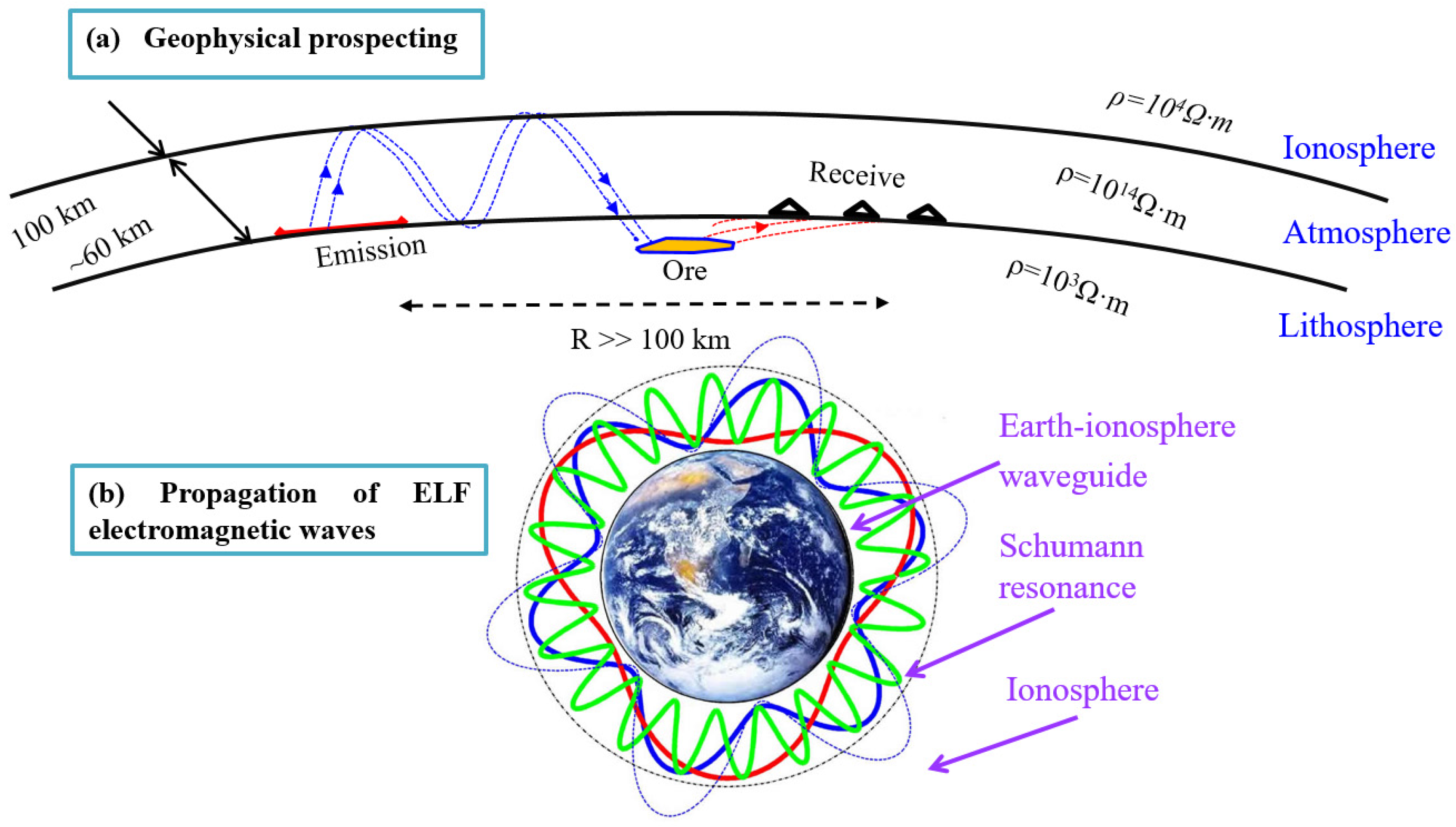
2.1. Spherical Earth–Ionosphere Model

To account for the spherical Earth and the ionosphere, the Earth–ionosphere waveguide model is depicted in Figure 2a. The excitation antenna is simplified to an electric dipole represented by its current moment $\widehat{x}Idl\delta \left(x\right)\delta \left(y\right)\delta \left(z-r_s\right)$, where $r_s=a+z_s$, $a$ is the Earth’s radius, and $z_s$ denotes the height of the dipole above the ground. The ionosphere is characterized by permeability ${\mu }_0$, relative permittivity ${\epsilon }_{-1}$, and conductivity ${\sigma }_{-1}$, and $h$ denotes the height of the lower boundary of the ionosphere. The air region is characterized by permeability ${\mu }_0$, uniform permittivity ${\epsilon }_0$, and conductivity ${\sigma }_1$. To study the ELF electromagnetic response of the Earth as a stack of layers of varying thickness and conductivity, the Earth region is considered to be composed of multiple concentric layers (Figure 2b), and the thickness of stratified Earth is $l_j$, the permeability ${\epsilon }_j$, and conductivity ${\sigma }_j$.

2.2. Debye Potentials

With the time-harmonic dependence of $e^{i\omega t}$, the wavenumbers of those regions are $k_j=\omega \sqrt{{\mu }_0\left({\epsilon }_j+i{\sigma }_j/\omega \right)}$, j = 2, 3, … N. In spherical coordinates, following the Maxwell equation, the field components are expressed in terms of the two Debye potentials $\psi$ and $U$ [14,37]: when $\psi =0$, the fields are referred to as transverse electric (TE) with respect to the radial direction; when $U=0$, the fields are referred to as transverse magnetic (TM) with respect to the radial direction. Therefore, Debye potentials for the functions in the ionospheric region are now written as:

$$TM:r{\psi }_{ino}=\cos \phi \cdot {\displaystyle \sum _{n=1}^{\infty }\left[E_n{\xi }_n\left(k_{ino}r\right)\right]P_n^1\left(\cos \theta \right)}$$

(1a)

$$TE:r{U}_{ino}=\sin \phi \cdot {\displaystyle \sum _{n=1}^{\infty }\left[F_n{\xi }_n\left(k_{ino}r\right)\right]P_n^1\left(\cos \theta \right)}$$

(1b)

When the source point is located on or near the Earth’s surface ($r_s=a+z_s$), the potential functions $\psi$ and $U$ in the air region should be expressed as:

$$TM:r{\psi }_1=\{\begin{array}{l}\cos \phi {\displaystyle \sum _{n=1}^{\infty }\left[\left({\alpha }_n+A_n\right){\chi }_n\left(k_{1}r\right)+B_n{\xi }_n\left(k_{1}r\right)\right]P_n^1\left(\cos \theta \right),r<r_s}\\ \cos \phi {\displaystyle \sum _{n=1}^{\infty }\left[A_n{\chi }_n\left(k_{1}r\right)+\left({\alpha }_n{}^{\prime }+B_n\right){\xi }_n\left(k_{1}r\right)\right]P_n^1\left(\cos \theta \right),r>r_s}\end{array}$$

(2a)

$$TE:r{U}_1=\{\begin{array}{l}\sin \phi {\displaystyle \sum _{n=1}^{\infty }\left[\left({\beta }_n+C_n\right){\chi }_n\left(k_{0}r\right)+D_n{\xi }_n\left(k_{1}r\right)\right]P_n^1\left(\cos \theta \right)},r<r_s\\ \sin \phi {\displaystyle \sum _{n=1}^{\infty }\left]C_n{\chi }_n\left(k_{1}r\right)+\left({\beta }_n{}^{\prime }{+D}_n\right){\xi }_n\left(k_{1}r\right)\right]P_n^1\left(\cos \theta \right)},r>r_s\end{array}$$

(2b)

Additionally, the potential function in the Earth region j should be expressed as:

$$TM:r{\psi }_j=\{\cos \phi {\displaystyle \sum _{n=1}^{\infty }\left[M_n{\chi }_n\left(k_{1}r\right)+G_n{\xi }_n\left(k_{1}r\right)\right]P_n^1\left(\cos \theta \right)}j=2,3,\dots ,N$$

(3a)

$$TE:r{U}_j=\{\sin \phi {\displaystyle \sum _{n=1}^{\infty }\left[N_n{\chi }_n\left(k_{1}r\right)+Q_n{\xi }_n\left(k_{1}r\right)\right]P_n^1\left(\cos \theta \right)}j=2,3,\dots ,N$$

(3b)

where $E_n, F_n, A_n, B_n, C_n, D_n, M_n, N_n, G_n$, and $Q_n$ represent the coefficients related to the electrical properties of the ionosphere and the Earth, ${\chi }_n\left(u\right)=u\cdot j_n\left(u\right)$ and ${\xi }_n\left(u\right)=u\cdot h_n^2\left(u\right)$ are Riccati–Bessel functions, ${\chi }_n\left(u\right)$ stands for standing wave, ${\xi }_n\left(u\right)$ stands for outward traveling wave, $P_n^1\left(\cos \theta \right)$ is the associated Legendre function, and ${\alpha }_n$ and ${\beta }_n$ [37] are the coefficients related to the nature of the source.

2.3. Determination of Coefficients

To make the tangential field components $E^{\theta }$, $E_{}^{\phi }$, $H_{}^{\theta }$, and $H_{}^{\phi }$ continuous [38] when across the element interfaces, it is sufficient to make the quantities of $\frac{1}{{\sigma }_j+i\omega \epsilon }\frac{\frac{\partial }{\partial r}\left(r{\psi }_j\right)}{r{\psi }_j}$ and $\frac{1}{i\omega \mu }\frac{\frac{\partial }{\partial r}\left(r{U}_j\right)}{r{U}_j}$ continuous. Thus, the spherical wave impedance [38] in the ionospheric region is:

$$TM:Z_{ic}^{\left(n\right)}=\frac{-k_{-1}}{{\sigma }_{-1}+i\omega \epsilon }\frac{{\xi }_n{}^{\prime }\left(k_{-1}c\right)}{{\xi }_n\left(k_{-1}c\right)}$$

(4a)

$$TE:Z_{ic}^{\left(n\right)*}=\frac{-k_{-1}}{{\sigma }_{-1}+i\omega \epsilon }\frac{{\xi }_n{}^{\prime }(k_{-1}r)}{{\xi }_n(k_{-1}r)}$$

(4b)

Additionally, in the air region,

$$TM:Z_{0c}^{\left(n\right)}=\frac{-k_1}{{\sigma }_1+i\omega \epsilon }\frac{A_n{\chi }_n{}^{\prime }(k_{1}c)+\left({\alpha }_n{}^{\prime }+B_n\right){\xi }_n{}^{\prime }(k_{1}c)}{A_n{\chi }_n(k_{1}c)+\left({\alpha }_n{}^{\prime }+B_n\right){\xi }_n(k_{1}c)}$$

(5a)

$$TE:Z_{0\mathrm{c}}^{\left(n\right)*}=\frac{-k_1}{i\omega \mu }\frac{C_n{\chi }_n{}^{\prime }\left(k_{1}c\right)+\left({\beta }_n{}^{\prime }+D_n\right){\xi }_n{}^{\prime }\left(k_{1}c\right)}{C_n{\chi }_n\left(k_{1}c\right)+\left({\beta }_n{}^{\prime }+D_n\right){\xi }_n\left(k_{1}c\right)}$$

(5b)

$$TM:Z_{0a}^{\left(n\right)}=\frac{k_1}{{\sigma }_1+i\omega \epsilon }\frac{\left({\alpha }_n+A_n\right){\chi }_n{}^{\prime }(k_{1}a)+B_n{\xi }_n{}^{\prime }(k_{1}a)}{\left({\alpha }_n+A_n\right){\chi }_n(k_{1}a)+B_n{\xi }_n(k_{1}a)}$$

(5c)

$$TE:Z_{0a}^{\left(n\right)*}=\frac{k_1}{i\omega \mu }\frac{\left({\beta }_n+C_n\right){\chi }_n{}^{\prime }\left(k_{1}a\right)+D_n{\xi }_n{}^{\prime }\left(k_{1}a\right)}{\left({\beta }_n+C_n\right){\chi }_n\left(k_{1}a\right)+D_n{\xi }_n\left(k_{1}a\right)}$$

(5d)

In the Earth region $j$, at the interface between the $jth$ layer and the $\left(j+1\right)th$ layer ($r=r_j$), the spherical wave impedance is rewritten as:

$$TM:Z_{ej\left(r_j\right)}^{\left(n\right)}=\frac{k_j}{{\sigma }_j+i\omega \epsilon }\frac{{\chi }_n{}^{\prime }(k_j{r}_j)+{\mathsf{\Delta }}_n^j{\xi }_n{}^{\prime }(k_j{r}_j)}{{\chi }_n(k_j{r}_j)+{\mathsf{\Delta }}_n^j{\xi }_n(k_j{r}_j)}$$

(6a)

$$TE:Z^{*}{}_{ej\left(r_j\right)}^{\left(n\right)}=\frac{k_j}{i\omega \mu }\frac{{\chi }_n{}^{\prime }(k_j{r}_j)+{\nabla }_n^j{\xi }_n{}^{\prime }(k_j{r}_j)}{{\chi }_n(k_j{r}_j)+{\nabla }_n^j{\xi }_n(k_j{r}_j)}$$

(6b)

and at the interface between layer $\left(j-1\right)th$ and layer $jth$($r=r_j$), we have:

$$TM:Z_{ej\left(r_{j-1}\right)}^{\left(n\right)}=\frac{k_j}{{\sigma }_j+i\omega \epsilon }\frac{{\chi }_n{}^{\prime }(k_j{r}_{j-1})+{\mathsf{\Delta }}_n^j{\xi }_n{}^{\prime }(k_j{r}_{j-1})}{{\chi }_n(k_j{r}_{j-1})+{\mathsf{\Delta }}_n^j{\xi }_n(k_j{r}_{j-1})}$$

(6c)

$$TE:Z^{*}{}_{ej\left(r_{j-1}\right)}^{\left(n\right)}=\frac{k_j}{i\omega \mu }\frac{{\chi }_n{}^{\prime }(k_j{r}_{j-1})+{\nabla }_n^j{\xi }_n{}^{\prime }(k_j{r}_{j-1})}{{\chi }_n(k_j{r}_{j-1})+{\nabla }_n^j{\xi }_n(k_j{r}_{j-1})}$$

(6d)

where ${\mathsf{\Delta }}_n^j=G_n^j/M_n^j$,${\nabla }_n^j=Q_n^j/N_n^j$. Since Equations (6a) and (6c), and (6b) and (6d) have the same undetermined coefficients, we have

$${\mathsf{\Delta }}_n^j=-\frac{Z_{ej\left(r_j\right)}^{\left(n\right)}{\chi }_n(k_j{r}_j)-\frac{k_j}{{\sigma }_j+i\omega \epsilon }{\chi }_n{}^{\prime }(k_j{r}_j)}{Z_{ej\left(r_j\right)}^{\left(n\right)}{\xi }_n(k_j{r}_j)-\frac{k_j}{{\sigma }_j+i\omega \epsilon }{\xi }_n{}^{\prime }(k_j{r}_j)}$$

(7a)

$${\nabla }_n^j=-\frac{Z^{*}{}_{ej\left(r_j\right)}^{\left(n\right)}{\chi }_n(k_j{r}_j)-\frac{k_j}{i\omega \mu }{\chi }_n{}^{\prime }(k_j{r}_j)}{Z^{*}{}_{ej\left(r_j\right)}^{\left(n\right)}{\xi }_n(k_j{r}_j)-\frac{k_j}{i\omega \mu }{\xi }_n{}^{\prime }(k_j{r}_j)}$$

(7b)

Substituting (7a) into (6a), and (7b) into (6b), we can obtain the impedance transformation relationship between two adjacent layers. For the layer N, coefficients G and Q in Equations (3a) and (3b) should be equal to zero because the field remains finite as r tends to zero, and we have:

$$Z_{eN-1\left(r_{N-1}\right)}^{\left(n\right)}=\frac{k_N}{{\sigma }_N+i\omega \epsilon }\frac{{\chi }_n{}^{\prime }(k_N{r}_{N-1})}{{\chi }_n(k_N{r}_{N-1})}$$

(8a)

$$Z^{*}{}_{eN-1\left(r_{N-1}\right)}^{\left(n\right)}=\frac{k_N}{i\omega \mu }\frac{{\chi }_n{}^{\prime }(k_N{r}_{N-1})}{{\chi }_n(k_N{r}_{N-1})}$$

(8b)

Starting from (8a) and (8b), the equivalent impedance $Z_{ea}^{\left(n\right)}$ and $Z_{e\left(a\right)}^{*\left(n\right)}$ of the Earth can be obtained layer by layer. Therefore, the boundary conditions [38] are transformed into:

$$\{\begin{array}{l}TM:\frac{-k_{ino}}{{\sigma }_{ino}+i\omega \epsilon }\frac{{\xi }_n{}^{\prime }\left(k_{ino}c\right)}{{\xi }_n\left(k_{ino}c\right)}=\frac{-k_1}{{\sigma }_1+i\omega \epsilon }\frac{A_n{\chi }_n{}^{\prime }\left(k_{1}r\right)+\left({\alpha }_n{}^{\prime }+B_n\right){\xi }_n{}^{\prime }\left(k_{1}r\right)}{A_n{\chi }_n\left(k_{1}r\right)+\left({\alpha }_n{}^{\prime }+B_n\right){\xi }_n\left(k_{1}r\right)}|{}_{r=c}\\ TE:\frac{-k_{ino}}{i\omega \mu }\frac{{\xi }_n{}^{\prime }\left(k_{ino}c\right)}{{\xi }_n\left(k_{ino}c\right)}=\frac{-k_1}{i\omega \mu }\frac{C_n{\chi }_n{}^{\prime }\left(k_{1}r\right)+\left({\beta }_n{}^{\prime }+D_n\right){\xi }_n{}^{\prime }\left(k_{1}r\right)}{C_n{\chi }_n\left(k_{1}r\right)+\left({\beta }_n{}^{\prime }+D_n\right){\xi }_n\left(k_{1}r\right)}|{}_{r=c}\end{array}$$

(9a)

$$\{\begin{array}{l}TM:Z_{ea}^{\left(n\right)}=\frac{k_1}{{\sigma }_1+i\omega \epsilon }\frac{\left({\alpha }_n+A_n\right){\chi }_n{}^{\prime }\left(k_{1}r\right)+B_n{\xi }_n\left(k_{1}r\right)}{\left({\alpha }_n+A_n\right){\chi }_n\left(k_{1}r\right)+B_n{\xi }_n\left(k_{1}r\right)}|{}_{r=a}\\ TE:Z^{*}{}_{ea}^{\left(n\right)}=\frac{k_1}{i\omega \mu }\frac{\left({\beta }_n+C_n\right){\chi }_n{}^{\prime }\left(k_{1}r\right)+D_n{\xi }_n\left(k_{1}r\right)}{\left({\beta }_n+C_n\right){\chi }_n\left(k_{1}r\right)+D_n{\xi }_n\left(k_{1}r\right)}|{}_{r=a}\end{array}$$

(9b)

The unknown coefficients and the expression of the electromagnetic field generated by the horizontal electric dipole source on the Earth’s surface are shown in Appendix A.

3. Convergence of Spherical Harmonic Series

Although the theory of spherical Earth models is physically better, it is slowly convergent due not only to series summation but also complicated mathematical functions. The convergence of infinite series in the EM field has always been a difficult point in the application, and the detailed and complete survey of the problems can be found in the works of the literature [26,39,40,41,42]. Since this work is interested in the physical concepts and the results that can reveal these concepts, the numerical calculation is not the focus. To compute the model field components, the continued fraction technique [43] is employed to speed up the computations, which has been proven useful in the calculation of the ELF-EM field. However, it needs to be pointed out that the algorithm cannot be employed to calculate the near field. Since the interest of this paper is to expand the application range of the WEM, and there are mature algorithms [24,31] for the calculation of near field, therefore, this algorithm is applicable to the problems discussed in this paper.

4. Verification

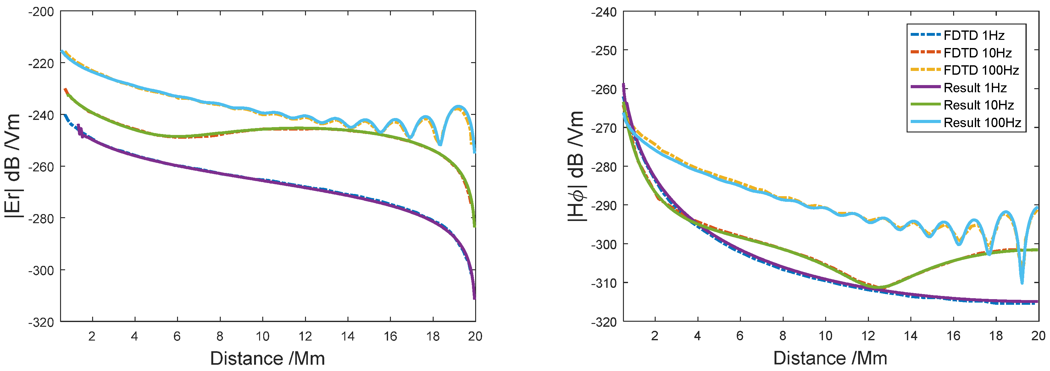
4.1. Comparison with FDTD

To verify the correctness and reliability of our formula and programming, with the same parameters, the results in the spherical “Earth–ionosphere” model are compared with the numerical simulation results of the finite difference time domain method (FDTD) [44]. The origin of the spherical coordinates is taken at the center of the Earth, the radius of the Earth is 6370 km, the location of the launch antenna is $\theta =0$, one end of the horizontal antenna is to $\phi =0$, and the other end points to $\phi =2\pi$. Assuming that both the dipole source and the observation point are located on the Earth’s surface, the excitation source is considered to be an electric current element $Idl=1A\cdot m$, the ionosphere height h = 70 km, the atmosphere conductivity is ${\sigma }_a={10}^{-14} \mathrm{S}/\mathrm{m}$, the Earth conductivity ${\sigma }_g={10}^{-4} \mathrm{S}/\mathrm{m}$, and the ionosphere conductivity ${\sigma }_i={10}^{-5} \mathrm{S}/\mathrm{m}$. Additionally, the magnitudes of the field components $\left|E_r\right|$ and $\left|H_{\phi }\right|$ versus the propagation distance are represented in Figure 3, where the transmission frequency is f = 1 Hz, 10 Hz, and 100 Hz. Furthermore, we provided spatial coverage that can constrain the EM field on the Earth’s surface in Figure 4.

It can be seen from Figure 3 that even in the nearby of the antipole of the dipole source (~20,000 km), the calculated results of our method are in good agreement with the numerical results of FDTD, indicating that the method proposed in this paper is correct. As stated earlier, the ELF-EM signals have sufficiently low attenuation to be received around the world, so there is the “interference” phenomenon of waves propagating along different paths [14,27]. This proved that the ELF-EM fields in the spherical cavity are standing waves. Compared with the signals of 1 Hz and 10 Hz, the signal of 100 Hz has a shorter wavelength and is more likely to be interfered in the cavity, resulting in an “interference” phenomenon, especially when the distance is greater than 8000 km. Different from the magnetic field component $\left|H_{\phi }\right|$, within the range of 8–12 Mm (1 Mm = 1 × 10⁶ m), the vertical electric component $\left|E_r\right|$ of 10 Hz is enhanced due to the superposition of signals of different paths, while the magnetic field component is rapidly weakened. In the range of 12–20 Mm, the electric field component decays rapidly and the magnetic field component increases. Figure 4 shows the spatial distribution of the vertical electric field at frequencies of 10 and 100 Hz. As discussed above, for 10 Hz, the radial component of the electric field has a maximum value near the equator, and at 100 Hz, there is an obvious “interference” phenomenon near the anti-polar region. In addition, it reveals that the field strength in the direction perpendicular to the transmitting antenna is the strongest, and the field strength along the antenna direction is the weakest.

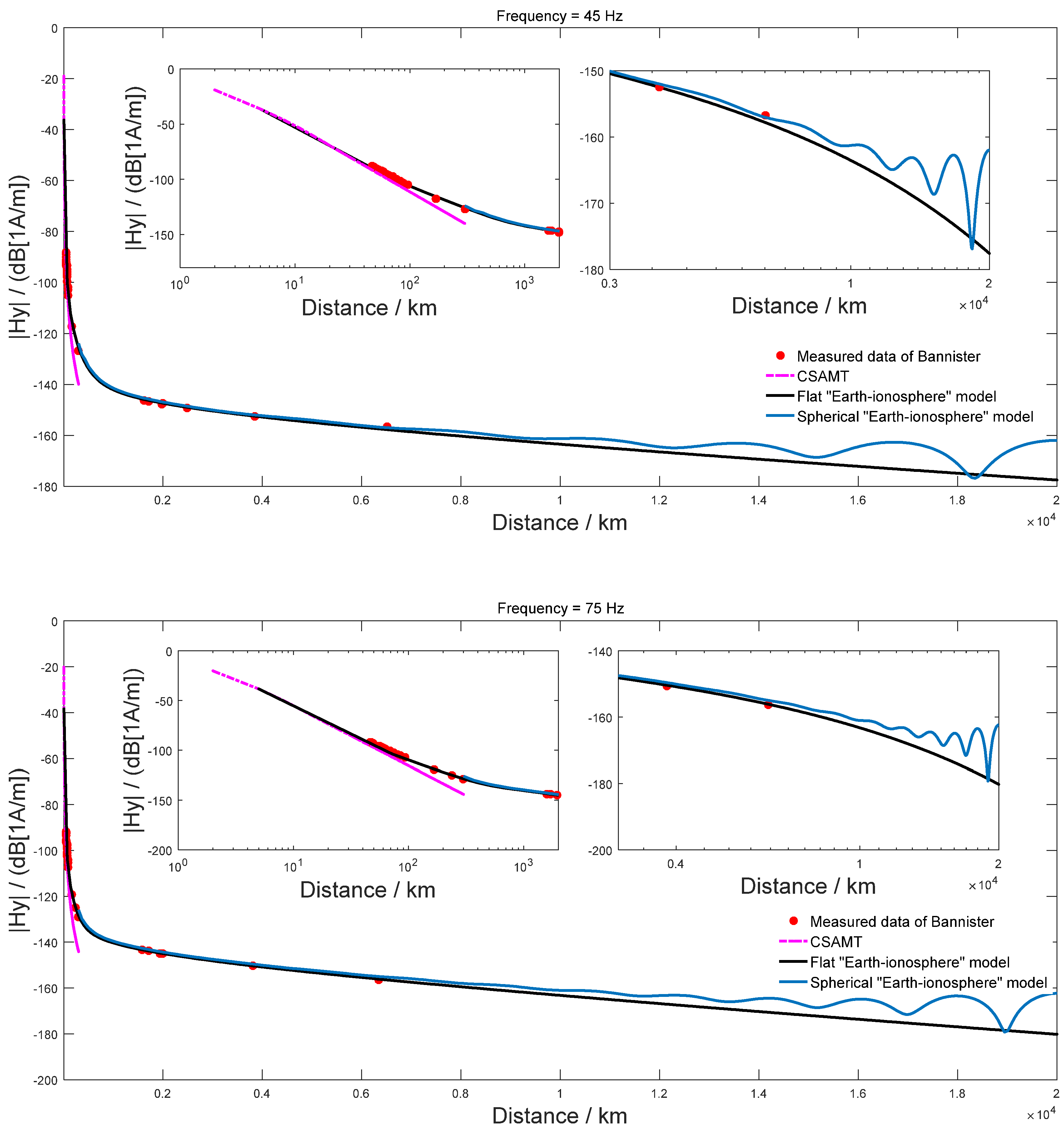
4.2. Comparison of CSAMT and WEM Methods

To illustrate the general behavior of the EM fields generated by artificial sources in the Earth–ionosphere cavity and to study the feasibility of the WEM for large-scale mineral exploration, the field components $\left|H\phi \right|$ of the spherical 1D Earth model were compared to controlled source audio-frequency magnetotelluric (CSAMT) and flat “Earth–ionosphere” models [24]. The calculations are based upon the Earth conductivities of 2.8 × 10⁻⁴ S·m at 45 Hz and 3.2 × 10⁻⁴ S·m at 75 Hz [13], with the conductivity of the atmosphere being 10⁻¹⁴ Ω·m, and the conductivity of ionosphere being 10⁻⁵ S·m. The horizontal antenna current is 300 A and the length is 22.5 km. Additionally, the height of the ionosphere is presented in Table 2 of reference [13]. The comparisons of the theoretical and experimental field strength are shown in Figure 5.

Clearly, when the transceiver distance is less than 10 km, the EM signals of WEM are agreed well with CASTM. At about 30 km, the attenuation of the CSAMT field accelerates and the curve deviates from the measured value. On the contrary, due to the consideration of ionospheric reflection, the WEM method is still in agreement with the measured ionosphere in the whole range of 6500 km. For the spherical model, when the transceiver distance is less than the radius of the Earth, the results are in good agreement with the plate model and the measured data. However, within the framework of spherical Earth models, the results of the spherical stratified model differ sensibly from that of the flat model. When the transceiver distance is larger than the radius of the Earth, only the spherical model results can show the interference of the field near the antipole of the dipole source, and its signal strength is much larger than that of the flat plate model. The above results suggest that it is necessary to consider the Earth curvature effect in long-distance and large-scale exploration, so as to provide theoretical support for practical data acquisition.

5. Numerical Simulations

Since our interest is the application in deep resource exploration, some simple models of the electrical conductivity structure of the lithosphere are given and their electromagnetic response is modeled. The purpose is to gain some insight into the behavior of the EM fields in the presence of conductive structures.

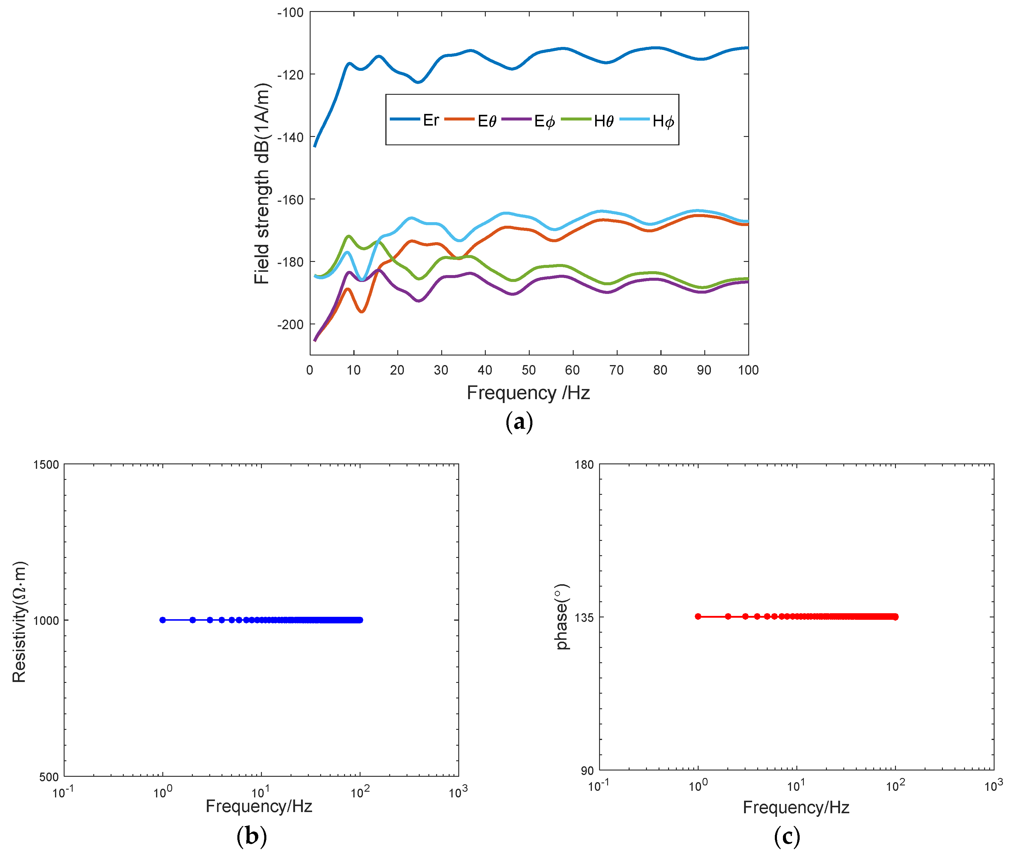
5.1. Response of a Homogeneous Earth

Figure 6 illustrates the general behavior of the EM fields generated by artificial sources in the Earth–ionosphere cavity. It shows the response of the fields as a function of transmitting frequency from 1 to 100 Hz and the observation azimuth is $\theta =2\pi /3$(~13.34 Mm). The calculations are based upon the antenna length of 100 km, the transmitting current 100 A [30], the Earth resistivity of ${10}^3\mathsf{\Omega }\cdot \mathrm{m}$, the resistivity of the atmosphere being 10¹⁴ $\mathsf{\Omega }\cdot \mathrm{m}$, and the resistivity of the ionosphere being ${10}^5\mathsf{\Omega }\cdot \mathrm{m}$.

It can be seen from Figure 6 that the amplitude of the radial electric field is much larger than that of other field components. The curves of $H_{\phi }$ and $E_{\theta }$($E_{\phi }$ and $H_{\theta }$) are closely connected near the value 7 Hz and increase rapidly. When the frequency is greater than 10 Hz, the field strengths of $E_{\theta }/H_{\phi }$ and $E_{\phi }/H_{\theta }$ have the same variation trend in the cavity, and they show harmonic oscillation. In the low-frequency band (<30 Hz), the amplitude of the magnetic field component is much larger than that of the electric field component. Interestingly, with the increase of frequency, the amplitudes of the electric field and magnetic field gradually increase and tend to be stable. Additionally, Figure 6 shows the apparent resistivity and phase response [45] when the transceiver distance is greater than the Earth radius (~13.34 Mm). It is apparent that in the ELF range, the apparent resistivity curve at different frequencies is completely coincident with the real resistivity of the Earth. Note that for a homogeneous Earth model, the phase is independent of the frequency and the electrical parameters of the media. From the definition of skin depth $\delta =\sqrt{2/\omega \mu \sigma }$, we know that the attenuation of the EM field is proportional to the square root of its working frequency, which reveals that the WEM (0.1–300 Hz) has great potential in the detection of the deep electrical structures of the Earth.

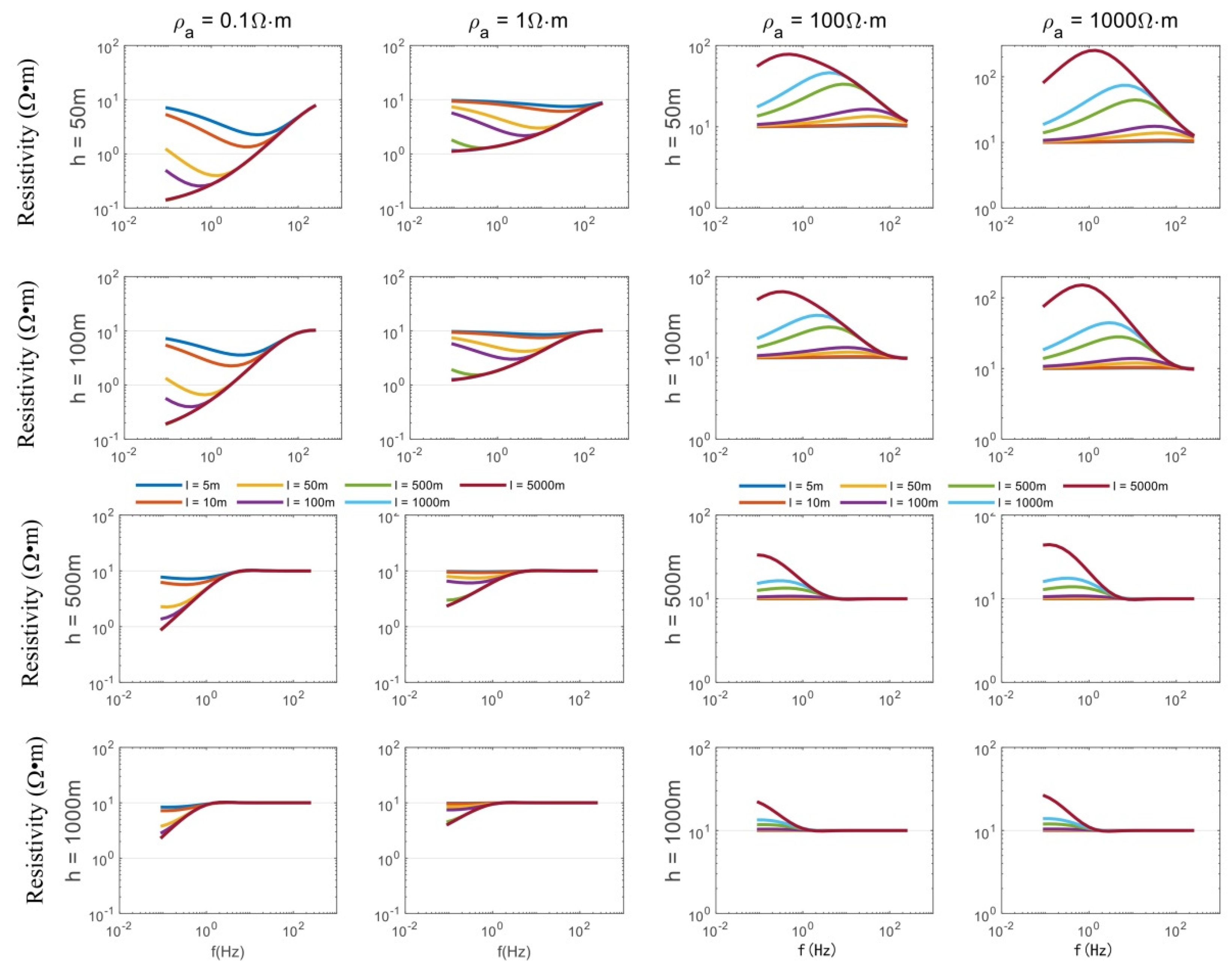
5.2. Sensitivity to a Thin Resistive Target

It is well known that the electrical properties of the ground affect the resolution of EM fields. In this section, key factors that could affect the EM field response, such as physical depth, thickness, and resistivity differences between the geological body and the surrounding rock, are discussed. The transmitting antenna is simplified as a horizontal electric dipole source. Figure 7 illustrates the resistivity behavior of a horizontal resistive layer imbedded in the homogeneous Earth with a background resistivity of 10 $\mathsf{\Omega }\cdot \mathrm{m}$, as observed in the waveguide region. The resistivity, thickness, and physical depth of the layer are varied in order to show the dependence of the responses on these parameters.

As shown in Figure 7, as the physical depth increases, at high frequencies, the high-frequency electromagnetic signal attenuates rapidly, and the apparent resistivity is equal to the resistivity of the top layer; at lower frequencies, apparent resistivity can reveal an amplitude anomaly caused by the target layer, and the maximum abnormal value of the curve moves to the low-frequency direction. In addition, the amplitude of the anomaly increases when the target layer becomes thicker, shallower, or more conductive. Note that Wannamaker (1983) pointed out that a resistive layer of a given contrast produces a lower anomalous intensity than a conductor of an equivalent contrast. Additionally, it can be found that as the ratio of the resistivity difference between the abnormal layer and the background layer decreases, the maximum abnormal amplitude of the apparent resistivity curve decreases.

It is worth noting that the apparent resistivity response of the HED is the same as that of the vertical electric dipole (VED) [38]. Following the resolution limit (Wannamaker, 1983), Zheng and Di (2021) depicted the maximum normalized anomaly curves for resistivity ratios of 0.01, 0.1, 1, 10, and 100 between the anomalous layer and the background layer, and pointed out that the resolution of the low-resistivity layer is highly dependent on the ratio of the resistivity, while the resistivity ratio has little effect on the resolution of the high-resistivity layer. That is, whether it is HED or VED, EM exploration is more sensitive to low-resistivity targets.

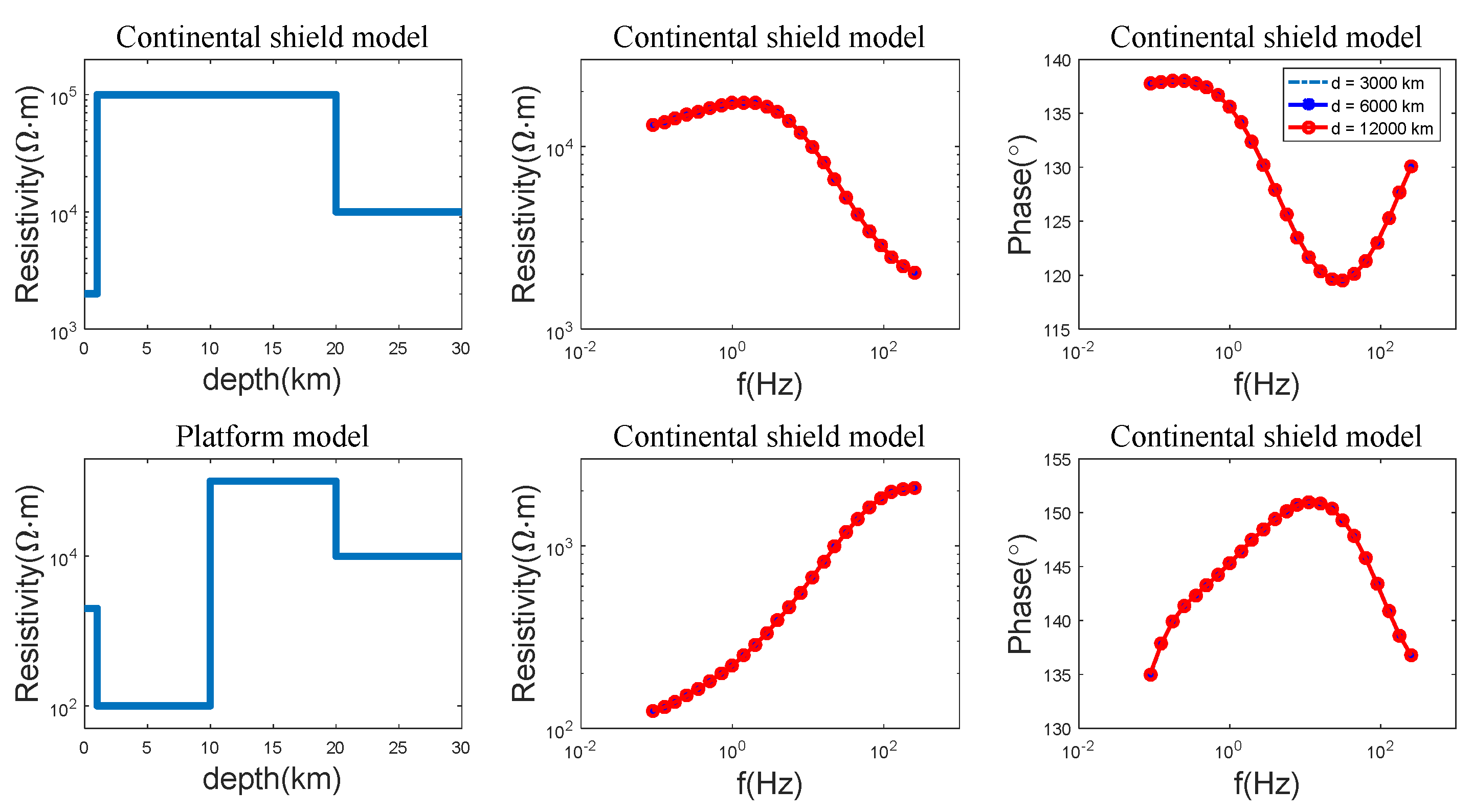
5.3. Forward Modeling of the Stratified Ground

In geophysics, it is often more interesting to model the Earth as a stack of layers of varying thickness and conductivity [36]. To study the EM properties of the layered media in the Earth–ionosphere mode, Figure 8 illustrates the resistivity and phase behavior of a two-layered Earth model with a target layer overlying an infinitely conductive basement, which is sufficient to illustrate the basic characteristics.

The coordinate system is the same as shown in Figure 2, the transmitting antenna is 100 km, the current is 100A, the transmission frequency is 2ⁿ Hz, n = −3.5:0.5:8, and the interval is 0.5. The height of the ionosphere is h = 70 km, and the resistivity of the ionosphere, air, and Earth layers are ${\rho }_{\mathrm{i}}={10}^5\mathsf{\Omega }\cdot \mathrm{m}$, ${\rho }_1={10}^{14}\mathsf{\Omega }\cdot \mathrm{m}$, ${\rho }_2={10}^2\mathsf{\Omega }\cdot \mathrm{m}$, and ${\rho }_3={10}^3\mathsf{\Omega }\cdot \mathrm{m}$, respectively. The thickness of the upper layer is taken to be l = 1000 m. The observation azimuth is $\phi =\pi /4$, and the distances from the source center are 3000 km, 6000 km, and 12,000 km, respectively. Additionally, the observation point and the transmitting antenna are both located on the ground surface.

It is known that the EM signals penetrate the Earth to a depth termed the skin depth, and as frequency decreases, the skin depth increases. The apparent resistivity can be considered as the average resistivity from the surface to the skin depth [46]. Both models shown in Figure 8 have the states of high resistance and low resistance, and the shape and amplitude of the apparent resistivity and phase response curves at different distances are the same. At high frequencies, the apparent resistivity is equal to the resistivity of the top layer; at lower frequencies, apparent resistivity is controlled by the basement. Note that due to the lack of high-frequency components, WEM needs to be combined with other EM methods such as the time-domain MTEM and SOTEM methods to achieve the effective detection of deep resources.

Furthermore, to better demonstrate the response characteristics of the EM field of the multilayer media, the frequency characteristics of the three-layered continental shield model and the four-layered platform model are simulated, which is enough to indicate the basic characteristics. For the continental shield model, the formation resistivity is: ${\rho }_2=2\times {10}^3\mathsf{\Omega }\cdot \mathrm{m}$, ${\rho }_3={10}^5\mathsf{\Omega }\cdot \mathrm{m}$, and ${\rho }_4={10}^4\mathsf{\Omega }\cdot \mathrm{m}$, and the thickness of each layer is: $l_2=1 \mathrm{km}$, $l_3=20 \mathrm{km}$, and $l_4=\infty$. For the platform model, the formation resistivity is: ${\rho }_2=2\times {10}^3\mathsf{\Omega }\cdot \mathrm{m}$, ${\rho }_3=100\mathsf{\Omega }\cdot \mathrm{m}$, ${\rho }_4={10}^5\mathsf{\Omega }\cdot \mathrm{m}$, and ${\rho }_5={10}^4\mathsf{\Omega }\cdot \mathrm{m}$, and the thicknesses of each layer are: $l_2=1\mathrm{km}$, $l_3=10 \mathrm{km}$, and $l_4=10 \mathrm{km}$, $l_5=\infty$, and other parameters are the same as in the two-layered model simulation.

As shown in Figure 9, for the given transmit and receive distance, the shape and amplitude of the apparent resistivity and phase response curves at different transmit and receive distances are basically the same. For the continental shield model, the existence of the crystalline shield layer with poor conductivity can be well shown as the frequency decreases. For the platform model, due to the influence of the low-resistance layer, the characteristics of the frequency response curve are completely different from those of the shield model. The field can reveal the existence of the middle conductive layer, but it is difficult to show the resistance status of the crystalline shield layer with poor conductivity. That is, when a thick geological layer of low resistivity is embedded in a high-resistivity background formation, it is difficult to distinguish the geological structure under the embedded layer. In this case, the resistivity response curve may lead to erroneous geological interpretation, which requires a comprehensive interpretation combined with other geophysical information.

6. Discussion and Conclusions

To extend the coverage of WEM to the global scale, we developed a spherical Earth–ionospheric waveguide model and derived the spherical harmonic expression of the ELF-EM field excited by a fixed high-power transmitter antenna. At first, the simulation results are compared with the FDTD in a full-space spherical model, which provides a good verification tool for the correctness of the spherical Earth–ionosphere theory. Then, we performed a detailed analysis of the effects of the Earth’s curvature on the ELF-EM fields. The analysis is carried out by comparing the flat and spherical models, which are notably different in their theoretical approaches and their methods of solution. It shows that when the offset is greater than the Earth’s radius, the effect of the Earth’s curvature on the ELF-EM fields is not negligible. When a spherical model is employed, the spatial ranges of EM waves are generally larger than that of the flat model. Then, the key factors that could affect the EM field response, such as physical depth, thickness, and resistivity differences between the geological body and the surrounding rock, are discussed. Additionally, the EM responses of some simple electrical conductivity structures models are modeled, which proves that WEM can provide a new solution for the division of fine resistivity structures in the lithosphere. Finally, some application cases of the ELF-EM field in geophysics are discussed to illustrate its prospects in future deep resource exploration.

Since any practical transmitter antenna will have an appreciable length, there will be errors in the dipole source model, and the next research work will focus on the fractional difference between dipole sources with the same moment and long wire.

References

1. Zhdanov, M.S. Geophysical Electromagnetic Theory and Methods; Elsevier: Amsterdam, The Netherlands, 2009. [Google Scholar]
2. Holzer, R.; Deal, O. Low audio-frequency electromagnetic signals of natural origin. Nature 1956, 177, 536–537. [Google Scholar] [CrossRef]
3. Lanzerotti, L.; Chave, A.; Sayres, C.; Medford, L.; Maclennan, C. Large-scale electric field measurements on the Earth’s surface: A review. J. Geophys. Res. Planets 1993, 98, 23525–23534. [Google Scholar] [CrossRef]
4. Dong, H.; Wei, W.; Jin, S.; Ye, G.; Jones, A.G.; Zhang, L.; Jing, J.e.; Xie, C.; Yin, Y. Shaping the Surface Deformation of Central and South Tibetan Plateau: Insights from Magnetotelluric Array Data. J. Geophys. Res. Solid Earth 2020, 125, e2019JB019206. [Google Scholar] [CrossRef]
5. Yu, N.; Unsworth, M.; Wang, X.; Li, D.; Wang, E.; Li, R.; Hu, Y.; Cai, X. New Insights into Crustal and Mantle Flow Beneath the Red River Fault Zone and Adjacent Areas on the Southern Margin of the Tibetan Plateau Revealed by a 3-D Magnetotelluric Study. J. Geophys. Res. Solid Earth 2020, 125, e2020JB019396. [Google Scholar] [CrossRef]
6. Fraser-Smith, A.C.; Bannister, P.R. Reception of ELF signals at antipodal distances. Radio Sci. 1998, 33, 83–88. [Google Scholar] [CrossRef] [Green Version]
7. Velikhov, E.; Zhamaletdinov, A.; Shevtsov, A.; Tokarev, A.; Kononov, Y.M.; Pesin, L.; Kadyshevich, G.; Pertel, M.; Veshchev, A. Deep electromagnetic studies with the use of powerful ELF radio installations. Izv. Phys. Solid Earth C/C Fiz. Zemli-Ross. Akad. Nauk. 1998, 34, 615–632. [Google Scholar]
8. Zhamaletdinov, A.; Shevtsov, A.; Korotkova, T.; Kopytenko, Y.A.; Ismagilov, V.; Petrishev, M.; Efimov, B.; Barannik, M.; Kolobov, V.; Prokopchuk, P. Deep electromagnetic sounding of the lithosphere in the Eastern Baltic (Fennoscandian) shield with high-power controlled sources and industrial power transmission lines (FENICS experiment). Izv. Phys. Solid Earth 2011, 47, 2–22. [Google Scholar] [CrossRef]
9. Bernstein, S.L.; Burrows, M.L.; Evans, J.E.; Griffiths, A.; McNeill, D.; Niessen, C.; Richer, I.; White, D.; Willim, D. Long-range communications at extremely low frequencies. Proc. IEEE 1974, 62, 292–312. [Google Scholar] [CrossRef]
10. Mosayebidorcheh, T.; Hosseinibalam, F.; Hassanzadeh, S. Analytical solution of electromagnetic radiation by a vertical electric dipole inside the earth and the effect of atmospheric electrical conductivity inhomogeneity. Adv. Space Res. 2017, 60, 1949–1957. [Google Scholar] [CrossRef]
11. Wait, J.R. Electromagnetic Waves in Stratified Media, 2nd ed.; Pergamon Press: New York, NY, USA, 1970; Volume 3. [Google Scholar]
12. Galejs, J. Terrestrial Propagation of Long Electromagnetic Waves: International Series of Monographs in Electromagnetic Waves; Elsevier: Amsterdam, The Netherlands, 2013; Volume 16. [Google Scholar]
13. Bannister, P.R.; Wolkoff, E.A.; Katan, J.R.; Williams, F. FarFarnal series of monographs in elecpagation measurements, 14 March to 9 April 1971. Radio Sci. 1973, 8, 623–631. [Google Scholar] [CrossRef]
14. Casey, J.P. Extremely Low Frequency (ELF) Propagation Formulas for Dipole Sources Radiating in a Spherical Earth-Ionosphere Waveguide; Naval Undersea Warfare Center: Newport, RI, USA, 2002. [Google Scholar]
15. Pan, W.; Li, K. Propagation of SLF/ELF Electromagnetic Waves; Springer Science & Business Media: Berlin/Heidelberg, Germany, 2013. [Google Scholar]
16. Lu, H.; Yang, J.; Li, Q.; Hao, S.; Guo, F.; Wu, J.; Chen, J.; Ma, G.; Xu, T. ELF/VLF communication experiment by modulated heating of ionospheric auroral electrojet at EISCAT. IEEE Trans. Antennas Propag. 2020, 69, 2267–2273. [Google Scholar] [CrossRef]
17. Pulinets, S.; Ouzounov, D. Lithosphere–Atmosphere–Ionosphere Coupling (LAIC) model–An unified concept for earthquake precursors validation. J. Asian Earth Sci. 2011, 41, 371–382. [Google Scholar] [CrossRef]
18. Nemec, F.; Santolik, O.; Parrot, M. Decrease of intensity of ELF/VLF waves observed in the upper ionosphere close to earthquakes: A statistical study. J. Geophys. Res. Atmos. 2009, 114, A04303. [Google Scholar] [CrossRef]
19. Asada, T.; Baba, H.; Kawazoe, M.; Sugiura, M. An attempt to delineate very low frequency electromagnetic signals associated with earthquakes. Earth Planets Space 2001, 53, 55–62. [Google Scholar] [CrossRef] [Green Version]
20. Zhamaletdinov, A.; Velikhov, E.; Shevtsov, A.; Kolobov, V.; Skorokhodov, A.; Ivonin, V.; Barannik, M.; Korotkova, T. Deep Electrical Conductivity of the Archaean Blocks of Kola Peninsula in the Light of the Results of Murman-2018 Experiment: A Review. Izv. Phys. Solid Earth 2021, 57, 61–83. [Google Scholar] [CrossRef]
21. Di, Q.; Xue, G.; Fu, C.; Wang, R. An alternative tool to controlled-source audio-frequency magnetotellurics method for prospecting deeply buried ore deposits. Sci. Bull. 2020, 65, 611–615. [Google Scholar] [CrossRef] [Green Version]
22. Qu, X.; Xue, B.; Fang, G. The propagation model and characteristics for extremely low frequency electromagnetic wave in Earth-ionosphere system and its application in geophysics prospecting. J. Electromagn. Waves Appl. 2018, 32, 319–331. [Google Scholar] [CrossRef]
23. Cao, M.; Tan, H.; Wang, K. 3D LBFGS inversion of controlled source extremely low frequency electromagnetic data. Appl. Geophys. 2016, 13, 689–700. [Google Scholar] [CrossRef]
24. Li, D.; Di, Q.; Wang, M.; Nobes, D. ‘Earth–ionosphere’mode controlled source electromagnetic method. Geophys. J. Int. 2015, 202, 1848–1858. [Google Scholar] [CrossRef]
25. Chandrasekhar, E. Regional electromagnetic induction studies using long period geomagnetic variations. In The Earth’s Magnetic Interior; Springer: Berlin/Heidelberg, Germany, 2011; pp. 31–42. [Google Scholar]
26. Barrick, D.E. Exact ULF/ELF dipole field strengths in the Earth-ionosphere cavity over the Schumann resonance region: Idealized boundaries. Radio Sci. 1999, 34, 209–227. [Google Scholar] [CrossRef]
27. Wang, Y.; Jin, R.; Geng, J.; Liang, X. Exact SLF/ELF underground HED field strengths in earth-ionosphere cavity and Schumann resonance. IEEE Trans. Antennas Propag. 2011, 59, 3031–3039. [Google Scholar] [CrossRef]
28. Cummer, S.A. Modeling electromagnetic propagation in the Earth-ionosphere waveguide. IEEE Trans. Antennas Propag. 2000, 48, 1420–1429. [Google Scholar] [CrossRef] [Green Version]
29. Simpson, J.J. Current and future applications of 3-D global earth-ionosphere models based on the full-vector Maxwell’s equations FDTD method. Surv. Geophys. 2009, 30, 105–130. [Google Scholar] [CrossRef]
30. Di, Q.; Fu, C.; Xue, G.; Wang, M.; An, Z.; Wang, R.; Wang, Z.; Lei, D.; Zhuo, X. Insight into skywave theory and breakthrough applications in resource exploration. Natl. Sci. Rev. 2021, 8, nwab046. [Google Scholar] [CrossRef]
31. Fu, C.; Di, Q.; Xu, C.; Wang, M. Electromagnetic fields for different type sources with effect of the ionosphere. Chin. J. Geophys. 2012, 55, 3958–3968. [Google Scholar]
32. Di, Q.; Wang, M.; Fu, C.; Li, D.; XU, C.; Zhuo, X. Study on the Propagation Characteristics of Electromagnetic Waves in the “Earth-Ionosphere” Mode; Science Press: Beijing, China, 2013. [Google Scholar]
33. Li, D.; Xie, W.; Di, Q.; Wang, M. Forward modeling for “earth-ionosphere” mode electromagnetic field. J. Cent. South Univ. 2016, 23, 2305–2313. [Google Scholar] [CrossRef]
34. Xu, Z.; Wu, X. Electromagnetic fields excited by the horizontal electrical dipole on the surface of the ionosphere-homogeneous earth model. Chin. J. Geophys. 2010, 53, 2497–2506. [Google Scholar]
35. Zhang, L. Research on Response of Full-Field Wiress Electromagnetic Method and 3D Intergral Equation Forward Modeling; Chinese Academy of Sciences: Beijing, China, 2021. [Google Scholar]
36. Chave, A.D.; Cox, C.S. Controlled electromagnetic sources for measuring electrical conductivity beneath the oceans: 1. Forward problem and model study. J. Geophys. Res. Solid Earth 1982, 87, 5327–5338. [Google Scholar] [CrossRef]
37. Xu, J.; Nie, Z. Scattering response of electromagnetic waves by multilayered spheres. Chin. J. Geophys. 1998, 865–876. [Google Scholar]
38. Zheng, F.; Di, Q. Propagation of ELF electromagnetic waves over a curved stratified ground and its application in geophysical prospecting. IEEE Access 2021, 9, 145563–145572. [Google Scholar] [CrossRef]
39. Ladutenko, K.; Pal, U.; Rivera, A.; Peña-Rodríguez, O. Mie calculation of electromagnetic near-field for a multilayered sphere. Comput. Phys. Commun. 2017, 214, 225–230. [Google Scholar] [CrossRef]
40. Wang, Y.; Jin, R.; Geng, J. Fast Convergence Algorithm for Earthquake Prediction Using SLF/ELF Horizontal Electric Dipole during Day and Night and Schumann Resonance. Wirel. Pers. Commun. 2012, 67, 149–163. [Google Scholar] [CrossRef]
41. Li, R.; Jiang, H.; Ren, K.F. Debye series for light scattering by a multilayered sphere. Appl. Opt. 2006, 45, 1260–1270. [Google Scholar] [CrossRef] [PubMed]
42. Kinayman, N.; Aksun, M. Comparative study of acceleration techniques for integrals and series in electromagnetic problems. Radio Sci. 1995, 30, 1713–1722. [Google Scholar] [CrossRef] [Green Version]
43. Zheng, F.; Di, Q.; Yun, Z.; Gao, Y. Convergence Acceleration of Infinite Series Involving the Product of Riccati–Bessel Function and Its Application for the Electromagnetic Field: Using the Continued Fraction Expansion Method. Appl. Comput. Electromagn. Soc. J. 2021, 36, 1518–1525. [Google Scholar]
44. Dong, H.; Yan, Y.; Li, Q. FDTD Simulation of SLF\ELF Fields Excited by Horizontal Electric Dipoles in Inhomogeneous Earth-Ionospheric Waveguides. Chin. J. Radio Sci. 2010, 25, 276–280. [Google Scholar] [CrossRef]
45. Zheng, F.; Di, Q.; Gao, Y.; Fu, C. Frequency response characteristics of WEM in seafloor. Chin. J. Geophys. 2021, 64, 2170–2183. [Google Scholar]
46. Unsworth, M. New developments in conventional hydrocarbon exploration with electromagnetic methods. CSEG Rec. 2005, 30, 34–38. [Google Scholar]
Figure 1. (a) Artificial electromagnetic signals reflected or refracted from the ionosphere back to the Earth’s surface; (b) brief model of the propagation of ELF-EM waves excited in Earth–ionospheric waveguide: the dotted line represents the lower boundary of the ionosphere, and the solid line represents the schematic diagram of the propagation paths of electromagnetic waves with different frequencies.
Remotesensing 14 03088 g001
Figure 2. (a) “Earth–ionosphere” waveguide model: the solid line represents the schematic diagram of the propagation paths of electromagnetic waves with different frequencies in the waveguide; (b) layered Earth model.
Remotesensing 14 03088 g002
Figure 3. Field components | E r | and | H φ | versus the propagation distance, where the solid line represents the result calculated by the FDTD, and the dashed line represents the results of this paper.
Remotesensing 14 03088 g003
Figure 4. Spatial distribution of field component | E r | (dB) at frequencies of f = 10 Hz and f = 100 Hz. Assuming that the transmitting antenna is placed at the North Pole, the calculations are based upon the antenna length of 100 km, the transmitting current 100 A, the Earth conductivity of 10 3   S / m , the conductivity of the atmosphere is 10 14   S / m , and the resistivity of the ionosphere is 10 5   S / m .
Remotesensing 14 03088 g004
Figure 5. Comparison of the amplitude and variation trend of the horizontal electromagnetic strength. The dots are the measurement data that Bannister obtained using the U.S. Navy ELF Wisconsin test facility, the dotted line is the result of CSAMT, the solid black line is the result of the plate model of reference [24], and the solid blue line is the result of the spherical cavity model in this paper.
Remotesensing 14 03088 g005
Figure 6. (a) Response of the EM fields generated by artificial sources in the Earth–ionosphere cavity as a function of transmitting frequency from 1 to 100 Hz and when the observation azimuth is θ = 2 π / 3 , and (b) apparent resistivity: ρ = 1 ω μ | E θ / H φ | 2 , (c) phase: ϕ = tan 1 ( Im ( E θ / H φ ) Re ( E θ / H φ ) ) .
Remotesensing 14 03088 g006
Figure 7. The electromagnetic response of a thin resistive target in the uniform Earth space; where ρ a is the resistivity (reciprocal of conductivity) of the layer, l is the thickness, and h is the buried depth.
Remotesensing 14 03088 g007
Figure 8. The apparent resistivity ρ = 1 ω μ | E θ / H φ | 2 and phases ϕ = tan 1 ( Im ( E θ / H φ ) Re ( E θ / H φ ) ) that are observed at the surface of a two-layered Earth Model G and Model D.
Remotesensing 14 03088 g008
Figure 9. Frequency responses of the continental shield model and platform model ( ρ = 1 ω μ | E θ / H φ | 2 , ϕ = tan 1 ( Im ( E θ / H φ ) Re ( E θ / H φ ) ) ), and the distances from the source center are 3000 km, 6000 km, and 12,000 km, respectively.
Remotesensing 14 03088 g009
Publisher’s Note: MDPI stays neutral with regard to jurisdictional claims in published maps and institutional affiliations.