An Improved Independent Parameter Decomposition Method for Gaofen-3 Surveying and Mapping Calibration

Abstract

The Gaofen-3 (GF-3) satellite can provide digital elevation model (DEM) data from its interferogram outputs. However, the accuracy of these data cannot be ensured without applying a surveying and mapping (SAM) calibration process, thus necessitating geometric and interferometric calibration technologies. In this paper, we propose an independent parameter decomposition (IPD) method to conduct SAM calibration on GF-3 data and generate high-accuracy DEMs. We resolved the geometric parameters to improve the location accuracy and resolved the interferometric parameters to improve the height accuracy. First, we established a geometric calibration model, analyzed the Range–Doppler (RD) model and resolved the initial imaging time error as well as the initial slant range error. Then, we established a three-dimensional reconstruction (TDR) model to analyze the height error sources. Finally, the interferometric phase error and baseline vector error were precisely estimated to ensure the vertical accuracy of the interferometric results by establishing the interferometric calibration model. We then used the GF-3 interferometric data derived on the same orbit in a north–south distribution to conduct the calibration experiment. The results show that the plane positioning accuracy was 5.09 m following geometric calibration, that the vertical accuracy of the interferometric results was 4.18 m following interferometric calibration and that the average absolute elevation accuracy of the derived DEM product was better than 3.09 m when using the GF-3 SAR data, thus confirming the correctness and effectiveness of the proposed GF-3 IPD calibration method. These results provide a technical basis for SAM calibration using GF-3 interferograms at the 1:50,000 scale in China.

1. Introduction

The Gaofen-3 (GF-3) satellite is the first civil C-band multipolarization synthetic aperture radar (SAR) satellite in China. This satellite has 12 imaging modes, including strip, spotlight and scanning modes. The image resolution ranges from 1 to 500 m, while the observation width ranges from 10 to 650 km. GF-3 can monitor global ocean and land information during all types of weather at all times and can expand the range of Earth observations through left–right attitude maneuvering. The satellite data can be used in many fields, such asoceanography, disaster reduction, water conservancy and meteorological and mapping research, to improve rapid response capabilities. This satellite has also filled the gap in civil autonomous high-resolution multipolarization SAR remote sensing data in China [1,2]. Topographic mapping is an important application direction in the field of remote sensing. Digital elevation model (DEM) data play important roles in national economic construction and scientific research [3,4]. Precise surveying and mapping (SAM) calibration technology has become one of the most effective means of global mapping; by incorporating SAR interferometry (InSAR) to acquire interferometric phase information of the land surface, high-precision elevation information is retrieved [5,6]. In 2000, the National Aeronautics and Space Administration (NASA), the National Imagery and Mapping Agency (NIMA) and the German Aerospace Center (DLR) jointly conducted the Shuttle Radar Topography Mission (SRTM), successfully completing approximately 80% of the proposed terrestrial topographic mapping mission on Earth; in addition, the absolute elevation accuracy of the DEM obtained by the SRTM was 16 m [7,8]. In 2016, the DLR acquired global TanDEM-X DEM data with an absolute elevation accuracy of 4 m; these data were improved over other global DEM data in their accuracy, thus introducing new opportunities for global topographic mapping [9]. In 2018, the DLR released global TanDEM-X DEM data at a 90 m grid size [10,11]. Therefore, obtaining global DEM data constitutes major engineering projects in the field of InSAR topographic mapping [11]. The abilities of high-precision satellite measurements in this application are important and depend not only on the design of the satellite platform index but also on the calibration of the geometric and interferometric parameters [6,12]. Geometric calibration steps improve the plane positioning accuracy of SAR images by calibrating the geometric parameters, while interferometric calibration technologies improve the vertical accuracy of the interferometric results by calibrating the acquired interferometric parameters [13,14]; together, these calibration steps can be used to determine the accuracy level of a global DEM. At present, many research teams in China and globally have published geometric and interferometric calibration methods that are applicable for mainstream SAR satellites [9,13,15].

After applying the geometric calibration method to the data obtained by the Japanese Advanced Land-Observing Satellite-Phased Array L-band SAR (ALSO-PALSAR), the geometric positioning accuracy of the strip mode reached 9.7 m [16]. A 5.74 m plane positioning accuracy was obtained for the Canada Radarsat-2 satellite after a geometric calibration method using corner reflectors (CRs) was applied [17]. German TerraSAR-X satellite data were subjected to high-precision geometric calibration with CRs and achieved a plane positioning result with an accuracy of 0.3 m [18]. In 2017, the geometric calibration precision of the GF-3 SAR satellite was studied, and the positioning accuracy was found to be better than 3 m [14]. In 2017, a multimode hybrid geometric calibration method was proposed for GF-3 images, and the geometric positioning accuracy was found to be better than 3 m [19]. In 2018, a sparse-control multiplatform geometric calibration method was proposed for TerraSAR-X/TanDEM-X and GF-3 images. The geometric positioning accuracy of the TerraSAR-X/TanDEM-X images found using this method was better than 3 m, while that of the GF-3 images was better than 7.5 m following calibration [15]. In 2020, a wide-area joint geometric calibration method was proposed for GF-3 SAR images, and the positioning error of the calibrated SAR images was better than 9 m [20]. Thus, this geometric calibration method has been successfully applied in engineering and scientific research in the past.

Although interferometric calibration technologies are complex, extensive research work has been conducted on this topic both in China and across the globe, and many interferometric calibration methods have been proposed. In 1999, an airborne interferometric calibration method based on a sensitivity equation was deduced using flat-ground geometric relationships [21]. In 2001, based on this research, an airborne interferometric calibration method was formulated based on the interferometric sensitivity equation under squint angle conditions [22]. In 2003, a three-dimensional reconstruction (TDR) model was introduced to derive the interferometric sensitivity equation, and a CR placement algorithm was proposed to minimize the condition numbers in sensitivity matrices [23]. In 2010, an airborne interferometric calibration model was proposed to accommodate the phase offset, baseline length and baseline angle [24]. Then, an airborne dual-antenna SAR interferometric calibration method based on the three-dimensional information of control points was proposed [25]. In 2011, a distributed satellite SAR interferometric altimetry model was proposed based on the TDR model [26]. An interferometric calibration optimization method for spaceborne distributed SAR systems was proposed to solve the problem of coupling the contribution of interferometric parameters to the elevation error [27]. In 2016, the interferometric calibration method derived based on the InSAR TDR model and sensitivity equation was verified using TanDEM-X data, thus proving the universality of this spaceborne SAR interferometric calibration method. However, in this technology verification, each error was not solved independently [28]. Table 1 further describes the current status of research on geometric and interferometric calibration methods.

Table 1. Research status of geometric calibration and interferometric calibration methods.

No.	Year	Authors	Description of the Method
1	2017	R. Zhao, G. Zhang, M. Deng [19]	A multimode hybrid geometric calibration method was proposed for GF-3 images, and the geometric positioning accuracy was found to be better than 3 m.
2	2018	LÜ Guannan, Tang Xinming, Ai Bo [15]	A sparse-control multiplatform geometric calibration method was proposed for Ter-raSAR-X/TanDEM-X and GF-3 images. The geometric positioning accuracy of the Ter-raSAR-X/TanDEM-X images found using this method was better than 3 m, while that of the GF-3 images was better than 7.5 m following calibration.
3	2020	DING Liujian, TAO Qiuxiang, LI Tao [20]	A wide-area joint geometric calibration method was proposed for GF-3 SAR images, and the positioning error of the calibrated SAR images was better than 9 m.
4	1999	Zink M, Geudtner D [21]	An airborne interferometric calibration method based on a sensitivity equation was deduced using flat-ground geometric relationships. The system parameters that were found to affect the interferometric elevation measurements were summarized, and the interferometric error sensitivity was analyzed.
5	2001	J. J. Mallorqui, M. Bara, and A. Broquetas [22]	An airborne interferometric calibration method was deduced based on the interferometric sensitivity equation under squint angle conditions. The simulation data confirmed that the condition numbers of different sensitivity matrices affect the interferometric calibration results differently; however, the identified corner reflector placement problem has not yet been explored.
6	2003	Wang Yanping [23]	A three-dimensional reconstruction (TDR) model was introduced to derive the interferometric sensitivity equation, and a CR placement algorithm was proposed to minimize the condition numbers in sensitivity matrices.
7	2010	Jin Guowang, Zhang Wei, Xiang Maosheng [24]	An airborne interferometric calibration model was proposed to accommodate the phase offset, baseline length and baseline angle, but the plane information of ground calibration points (GCPs) was not considered in this model.
8	2010	Zhang Wei, Xiang Maosheng, Wu Yirong [25]	An airborne dual-antenna SAR interferometric calibration method based on the three-dimensional information of control points was proposed, and this method could verify the plane and elevation accuracies of a DEM following calibration; however, the correction of each interferometric parameter was not solved independently in this method.
9	2011	HU Jiwei, Hong Jun [26]	A distributed satellite SAR interferometric altimetry model was proposed based on the TDR model, and the characteristics of the baseline vector and phase error were analyzed using simulated data.
10	2011	Zhang Yongjun [27]	An interferometric calibration optimization method for spaceborne distributed SAR systems was proposed to solve the problem of coupling the contribution of interferometric parameters to the elevation error. The simulated results showed that the method was feasible, but the existing research on each error factor has not been sufficiently deep, and studies analyzing measured supporting data have been lacking.
11	2016	Wu Danqin [28]	The interferometric calibration method derived based on the InSAR TDR model and sensitivity equation was verified using TanDEM-X data, thus proving the universality of this spaceborne SAR interferometric calibration method. However, in this technology verification, each error was not solved independently.

To date, geometric calibration technologies have gradually matured, and interferometric calibration technologies have developed from airborne to spaceborne systems. 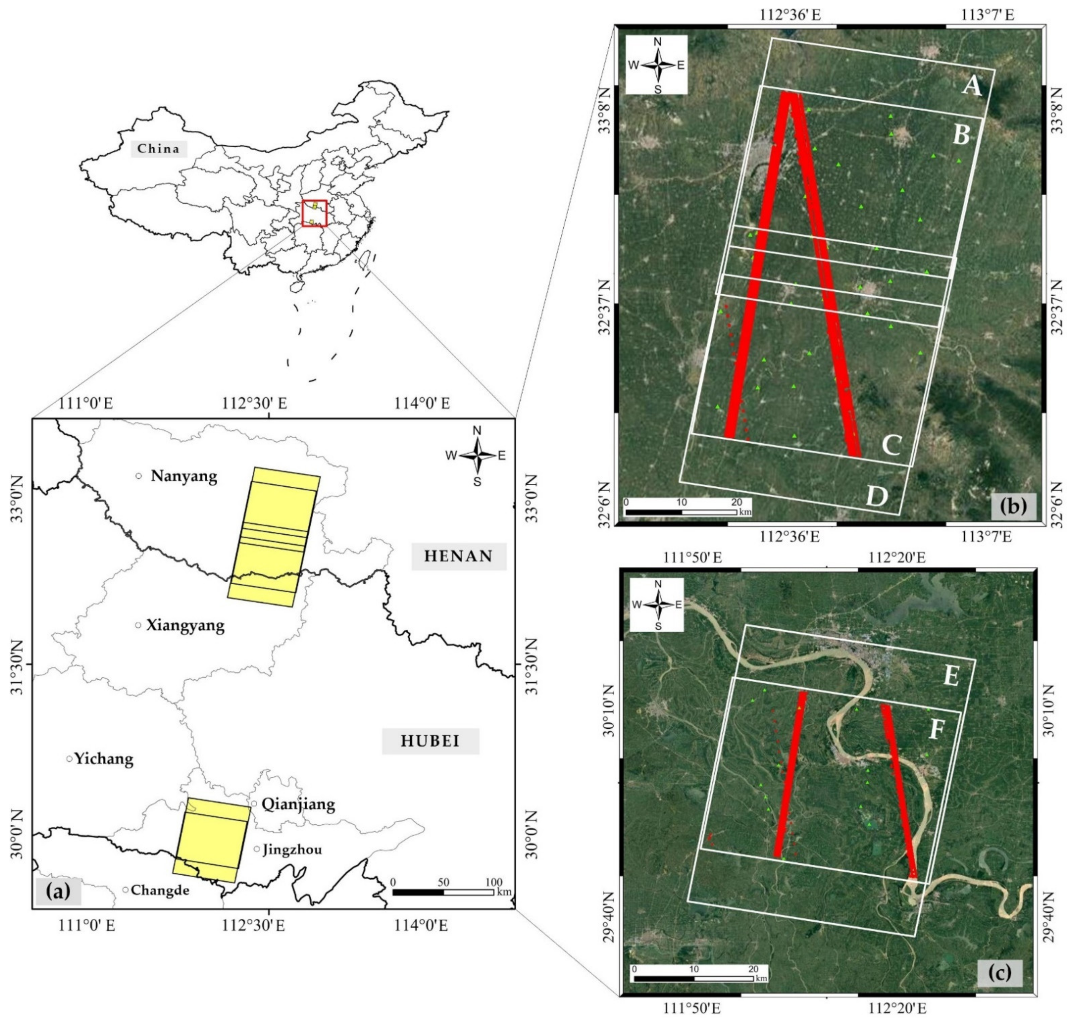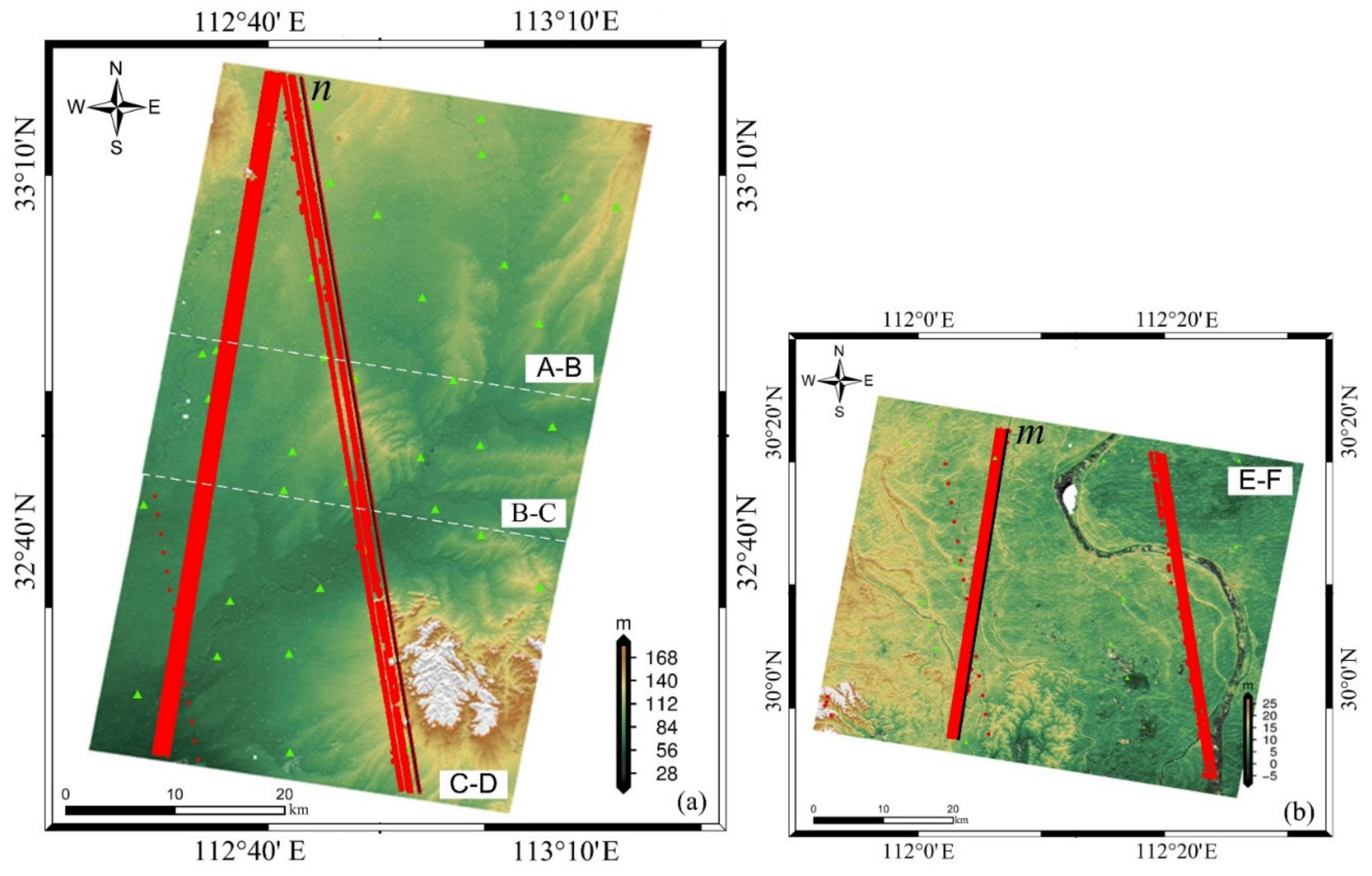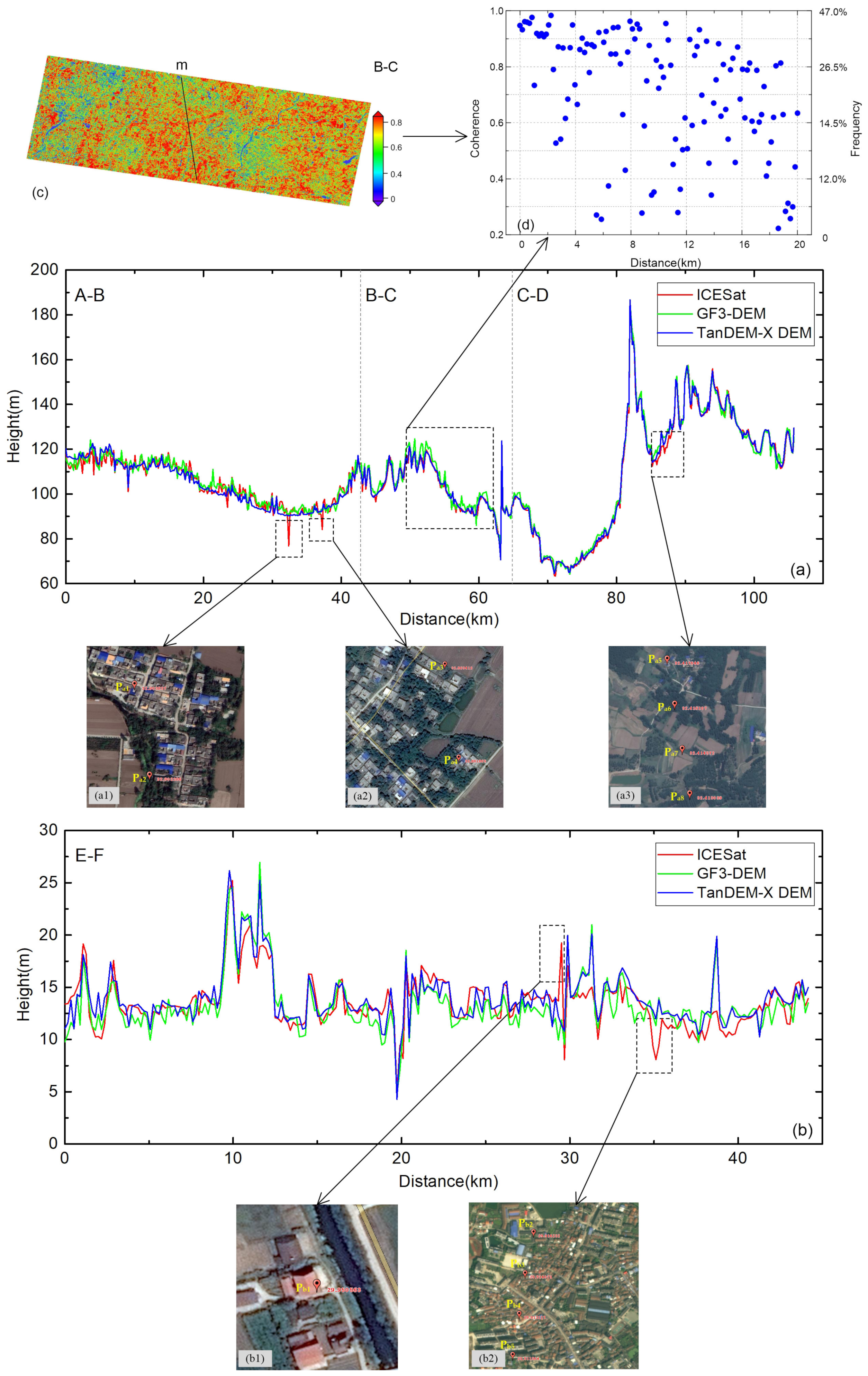Although extensive research has been conducted on this topic, most analyzed parameter errors exhibit strong coupling effects during the interference process, and no joint solution has been accurately distinguished, leading to inaccurate interferometric parameter corrections [28]. To solve this problem, a precise SAM calibration method is proposed herein based on independent parameter decomposition (IPD). We established a geometric calibration model and resolved the initial imaging time error as well as the initial slant range error to improve the location accuracy. On this basis, the interferometric phase error and baseline vector error were precisely estimated to ensure the vertical accuracy of the interferometric results by establishing the interferometric calibration model. The accuracy and reliability of the proposed method were verified by processing GF-3 SAR data obtained on the same orbit in six scenes, and high-accuracy DEM products were obtained, thus providing a technical reference for the global mapping missions of domestic SAR satellites.

2. Geometric Calibration Model

Due to the measurement errors of satellite orbit and imaging parameters, the plane positioning accuracy of SAR images is always restricted. Geometric calibration technologies are the key to achieving high-precision SAR image positioning information and are also the main method by which the generation of high-precision DEMs can be ensured. The Range–Doppler (R-D) model, the mainstream positioning model used for SAR geometry processing, is a rigorous model that conforms to the SAR imaging mechanism and describes the geometric relationships between satellite sensors and object points in the geocentric coordinate system. The R-D model is a nonlinear system of equations composed of the slant range equation, Doppler equation and Earth ellipsoid equation; these three equations can be expressed as follows [15]:

$$R_1=\left|{\overrightarrow{S}}_1-\overrightarrow{P}\right|$$

(1)

$$f_{dop}=-\frac{2}{\lambda }\frac{\left({\overrightarrow{S}}_1-\overrightarrow{P}\right)\cdot \left({\overrightarrow{v}}_{\mathrm{s}}-{\overrightarrow{v}}_t\right)}{R_1}$$

(2)

$$\frac{X_t^2+Y_t^2}{{\left(R_e+H_t\right)}^2}+\frac{Z_t^2}{R_p^2}=1$$

(3)

where $R_1$ is the distance between the main satellite sensor and the ground object, ${\overrightarrow{S}}_1={\left(X_{\mathrm{s}},Y_s,Z_s\right)}^{\mathrm{T}}$ is the position vector of the satellite sensor, $\overrightarrow{P}={(X_t,Y_t,Z_t)}^{\mathrm{T}}$ is the position vector of the ground object, $f_d{}_{op}$ is the Doppler frequency, $\lambda$ is the radar wavelength, ${\overrightarrow{v}}_{\mathrm{s}}={\left(V_{\mathrm{x}},V_y,V_z\right)}^{\mathrm{T}}$ is the velocity vector of the satellite sensor and ${\overrightarrow{v}}_t$ is the velocity vector of the ground object. Because the ground object point is located on the Earth ellipsoid, the velocity vector of the ground object point in the geocentric coordinate system is 0; that is, ${\overrightarrow{v}}_t=0$. $R_e$ and $R_p$ are the major semiaxes and minor semiaxes of the Earth reference ellipsoid, respectively, and $H_t$ is the elevation of the ground object.

The position and velocity vectors of the satellite sensor can be described as functions of time using cubic polynomials, as shown in Formula (4).

$$\left\{\begin{array}{c}{X}_{\mathrm{s}}=a_0+a_{1}t+a_2{t}^2+a_3{t}^3\\ Y_{\mathrm{s}}=b_0+b_{1}t+b_2{t}^2+b_3{t}^3\\ Z_{\mathrm{s}}=c_0+c_{1}t+c_2{t}^2+c_3{t}^3\end{array}\begin{array}{c}\begin{array}{cc}& \\ & \end{array}\\ \end{array}\right.\left\{\begin{array}{c}{V}_x=a_1+2a_{2}t+3a_3{t}^2\\ V_y=b_1+2b_{2}t+3b_3{t}^2\\ V_{\mathrm{z}}=c_1+2c_{2}t+3c_3{t}^2\end{array}\right.$$

(4)

According to the R-D positioning model, the variables that are necessary for geometric positioning include the slant range (R), satellite sensor position vector (${\overrightarrow{S}}_1={\left(X_{\mathrm{s}},Y_s,Z_s\right)}^{\mathrm{T}}$), satellite sensor velocity vector (${\overrightarrow{v}}_{\mathrm{s}}={\left(V_{\mathrm{x}},V_y,V_z\right)}^{\mathrm{T}}$), Doppler frequency ($f_d{}_{op}$), radar wavelength ($\lambda$) and ellipsoid parameters ($Re/Rp$). Among them, the radar wavelength is a known value that can be obtained according to the formula $\lambda =c/f$, where c is the speed of light and f is the frequency. The ellipsoid parameters can also be obtained after the ellipsoid model is selected.

The slant range can be obtained by measuring the temporal difference between the transmission and reception of the radar pulse; the slant range error causes the position of the field of view of the target to move along the Doppler line, thus resulting in a positioning error. In the geometric positioning model, the slant range can be expressed as a linear function of the image column number as follows:

$$R_1=r_0+m_j\cdot j$$

(5)

where $r_0$ is the initial slant range, $m_j$ is the range pixel spacing and $j$ is the range pixel coordinate. In Equation (5), only the effect of the initial slant range error is considered when assessing the positioning accuracy in the range direction.

The linear function between the azimuth direction time and image line number can be expressed as follows:

$$t=t_0+t_1\cdot i$$

(6)

where $t_0$ is the initial imaging time, $t_1$ is the azimuth time spacing and $i$ is the line number of the image along the azimuth. Equation (6) considers only the effect of the initial imaging time error on the positioning accuracy in the azimuth direction.

In summary, we consider only the impacts of the initial slant range and imaging time on the plane positioning accuracy, so the geometric calibration parameters of interest in this paper are $(r_0,t_0)$. Then, the geometric calibration model is established according to the R-D model, and the geometric calibration parameters are estimated.

First, a conditional equation based on the slant range equation is established as follows:

$$F_1=\left|{\overrightarrow{S}}_1-\overrightarrow{P}\right|-\left(r_0+m_j\cdot j\right)$$

(7)

Next, a conditional equation based on the Doppler frequency is established as follows:

$$F_2=-\frac{2}{\lambda }\cdot \frac{\left({\overrightarrow{S}}_1-\overrightarrow{P}\right)\cdot \overrightarrow{v}}{R_1}$$

(8)

Then, the geometric calibration parameters are estimated using the nonlinear least squares method by considering several calibration points derived based on the conditional equation. The calibration parameter $(r_0,t_0)$ is used as an unknown observation value, and the error equation is obtained by linearizing the observation value derivation; these equations can be expressed as follows:

$$\left\{\begin{array}{l}{V}_1=\frac{\partial F_1}{\partial r_0}\Delta r_0+\frac{\partial F_1}{\partial t_0}\Delta t_0+{\left(F_1\right)}^0-F_1\\ V_2=\frac{\partial F_2}{\partial r_0}\Delta r_0+\frac{\partial F_2}{\partial t_0}\Delta t_0+{\left(F_2\right)}^0-F_2\end{array}\right.$$

(9)

where the true observation value is $F_1=F_2=0$. The observation errors ${\left(F_1\right)}^0$ and ${\left(F_2\right)}^0$ can be calculated by substituting approximate values of each undetermined geometric calibration parameter $(r_0,t_0)$ into Equations (7) and (8), respectively. The error equation can be rewritten as a matrix and expressed as follows:

$$V=BX-L$$

(10)

where $V=\left[\begin{array}{l}{V}_1\\ V_2\end{array}\right]$, $B=\left[\begin{array}{cc}\frac{\partial F_1}{\partial r_0}& \frac{\partial F_1}{\partial t_0}\\ \frac{\partial F_2}{\partial r_0}& \frac{\partial F_2}{\partial t_0}\end{array}\right]$, $X=\left[\begin{array}{l}\Delta r_0\\ \Delta t_0\end{array}\right]$ and $L=\left[\begin{array}{l}-{\left(F_1\right)}^0\\ -{\left(F_2\right)}^0\end{array}\right]$.

The coefficients in matrix B are derived from the partial derivatives of Equations (7) and (8) to obtain the geometric calibration parameter $(r_0,t_0)$, which can be expressed as follows:

$$\left\{\begin{array}{l}\frac{\partial F_1}{\partial r_0}=-1\hfill \\ \frac{\partial F_1}{\partial t_0}=\frac{K}{R^2}\left(Q_{1}R-\frac{M{Q}_2}{R}\right)\hfill \\ \frac{\partial F_2}{\partial r_0}=0\hfill \\ \frac{\partial F_2}{\partial t_0}=\frac{Q_2}{R}\hfill \end{array}\right.$$

(11)

where $K=-2/\lambda$, $M=X_v\left(X_s-X_t\right)+Y_v\left(Y_s-Y_t\right)+Z_v\left(Z_s-Z_t\right)$, and

$$\begin{array}{l}{Q}_1=X_v\left(a_1+2a_{2}t+3a_3{t}^2\right)+\left(X_s-X_t\right)\cdot \left(2a_2+6a_{3}t\right)+Y_v\left(b_1+2b_{2}t+3b_3{t}^2\right)+\left(Y_s-Y_t\right)\cdot \left(2b_2+6b_{3}t\right)+\\ Z_v\left(c_1+2c_{2}t+3c_3{t}^2\right)+\left(Z_s-Z_t\right)\cdot \left(2c_2+6c_{3}t\right)\\ Q_2=\left(X_s-X_t\right)\cdot \left(a_1+2a_{2}t+3a_3{t}^2\right)+\left(Y_s-Y_t\right)\cdot \left(b_1+2b_{2}t+3b_3{t}^2\right)+\left(Z_s-Z_t\right)\cdot \left(c_1+2c_{2}t+3c_3{t}^2\right)\end{array}$$

Finally, the normal equation can be established based on the initial value ($X_0$) of the geometric parameter.

$$B^{T}BX-B^{T}L=0$$

(12)

The geometric correction parameter can then be corrected based on the normal equation; the result can be written as follows:

$$\Delta X={\left(B^{T}B\right)}^{-1}{B}^{T}L$$

(13)

The first geometric calibration parameter estimation can be obtained as follows:

$$X=X_0+X$$

(14)

The geometric correction parameter solution is obtained in a gradual iterative approach process. First, the initial values of calibration parameters $r_0$ and $t_0$ are obtained; then, the error equation is established according to these initial values, and the geometric calibration parameter is corrected using the normal equation. Next, the first approximate value of the calibration parameter is obtained, and this value is taken as the initial value in the next iteration. When the calibration parameter gradually stabilizes after many iterations and the parameter correction is less than the specified threshold ($\epsilon ={10}^{-6}$), the iteration is said to have converged. At this time, the cumulative parameter correction result is considered to be the final error in the geometric calibration parameters.

3. Three-Dimensional Reconstruction Model

The TDR is the basic model applied to spaceborne InSAR. Its basic principle involves obtaining the three-dimensional coordinates of GCPs by combining the slant range equation and Doppler equation in the R-D positioning model through the interferometric equation [29].

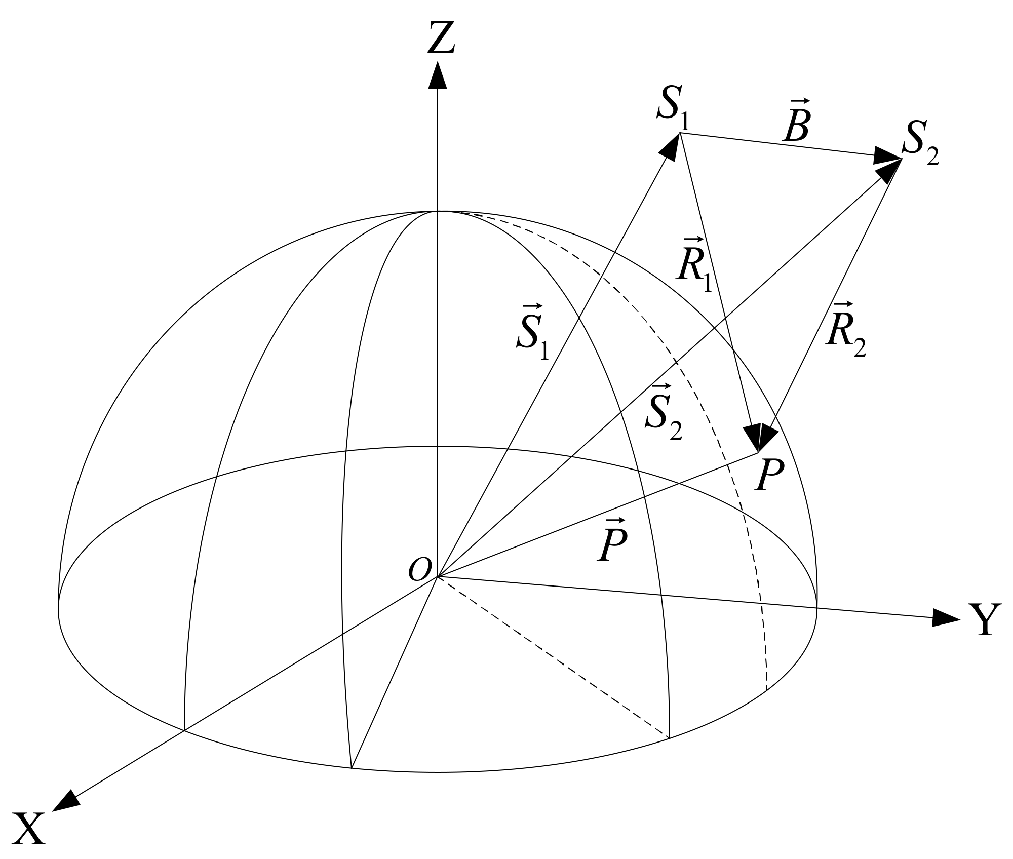
Herein, we describe the geometric relationship of the InSAR data in geocentric space rectangular coordinates (O-XYZ), as shown in Figure 1, where $S_1$ and $S_2$ are satellites; ${\overrightarrow{R}}_1$ and ${\overrightarrow{R}}_2$ are the position vectors of the satellite to the GCP; $\overrightarrow{P}$ is the position vector of the GCP; $R_1$ and $R_2$ are the slant ranges of $S_1$ and $S_2$, respectively; $\overrightarrow{v}$ is the velocity vector; $f_{dop}$ is the Doppler frequency; $\lambda$ is the radar wavelength; $\phi$ is the absolute phase; $\varphi$ is the wrapped phase; $B$ is the baseline vector; and $Q$ is the antenna receiving mode. The Q values of 2 and 1 represent the repeated-orbit interferometric mode and the double-antenna interferometric mode, respectively.

Figure 1. Geometric relationships of the spaceborne InSAR.

We mainly focus on the cross-track interferometry (XTI) mode of the spaceborne InSAR. The slant range equation, the Doppler equation in the R-D model and the interferometric phase equation are combined to establish the TDR model, and the geometric relationships can be expressed as follows:

$$R_1=\left|{\overrightarrow{S}}_1-\overrightarrow{P}\right|$$

(15)

$$f_{dop}=-\frac{2}{\lambda }\frac{\left({\overrightarrow{S}}_1-\overrightarrow{P}\right)\cdot \left({\overrightarrow{v}}_{\mathrm{s}}-{\overrightarrow{v}}_t\right)}{R_1}$$

(16)

$$\phi =\varphi +2k\pi =\frac{2\pi Q(R_1-R_2)}{\lambda }$$

(17)

According to the geometric relationships of the interferometric SAR, the GCP can be expressed in O-XYZ coordinates as follows:

$$\overrightarrow{P}={\overrightarrow{S}}_1+{\overrightarrow{R}}_1={\overrightarrow{S}}_1+R_1\cdot \widehat{r}$$

(18)

where ${\overrightarrow{R}}_1$ is the look vector and $\widehat{r}$ is the unit look vector. In Equation (18), the look vector decomposition (LVD) method is generally used to obtain the GCP coordinates. In this work, we convert the look vector to the unit look vector during the calculation [29], and the unit look vector needs to be represented in the Madsen moving coordinate (MMC) system [30]. The MMC system is based on applying the phase center of the main antenna as the origin of the coordinate system; the velocity vector direction is set to be equal to the V axis; the velocity and baseline cross product direction are set to be equal to the W axis; and V, N and W are set to meet the requirements of the right-hand coordinate system. To more conveniently describe the system, we refer to the MMC system as VNW in this work. The terms $r_v$, $r_n$ and $r_w$ are considered components of the unit look vector on the V, N and W axes, respectively, and $\widehat{r}$ can be written as follows:

$$\widehat{r}=\left[\begin{array}{l}{r}_v\\ r_n\\ r_w\end{array}\right]$$

(19)

In the LVD method, the look vector is converted from VNW coordinates to O-XYZ coordinates to obtain the three-dimensional coordinates of the GCPs, as shown in Equation (20) below:

$$\begin{array}{cc}\hfill & \overrightarrow{P}={\overrightarrow{S}}_1+{\overrightarrow{R}}_1={\overrightarrow{S}}_1+R_1·T_{vnw}^{-1}·{\widehat{r}}_{vnw}\hfill \\ \hfill & ={\overrightarrow{S}}_1+R_1·\left[\frac{\overrightarrow{v}}{\left|\overrightarrow{v}\right|},\frac{\left(\overrightarrow{v}\otimes \overrightarrow{B}\right)\otimes \overrightarrow{v}}{\left|\left(\overrightarrow{v}\otimes \overrightarrow{B}\right)\otimes \overrightarrow{v}\right|},\frac{\left(\overrightarrow{v}\otimes \overrightarrow{B}\right)}{\left|\left(\overrightarrow{v}\otimes \overrightarrow{B}\right)\right|}\right]\left[\begin{array}{c}\frac{\lambda f_{dop}}{2\left|\overrightarrow{v}\right|}\hfill \\ \frac{R_1}{2\left|b_{pv}\right|}\left[1+\frac{{\left|\overrightarrow{B}\right|}^2}{R_1^2}-{\left(1-\frac{\lambda \phi }{2\pi Q{R}_1}\right)}^2\right]-\frac{b_v{r}_v}{\left|b_{pv}\right|}\hfill \\ \pm \sqrt{1-r_v^2-r_n^2}\hfill \end{array}\right]\hfill \end{array}$$

(20)

where $T_{vnw}^{-1}$ is the transformation matrix, $b_v$ is the baseline component in the velocity direction and $b_{pv}$ is the baseline component in the direction perpendicular to the velocity.

According to the TDR expression, the main factors that affect the precision of interferometric SAR data are the interferometric phase error and the baseline vector error. Due to coupling among interferometric parameter error sources, to improve the accuracy of the interferometric parameter calculations during the calibration process, we adopted the IPD method, thus allowing us to precisely estimate the interferometric phase error and baseline vector error, improve the vertical accuracy of interferometric results and ultimately obtain high-precision DEM products.

4. Interferometric Calibration Model

The method utilized in this paper is based on the transmission characteristics of the interferometric phase error and baseline vector error to the elevation error; these characteristics are used herein to establish the interferometric calibration model. In spaceborne InSAR topographic mapping, interferometric phase errors generally consist of random and systematic errors. The random errors are caused by incoherent sources in the InSAR system, and the corresponding phases are randomly distributed; these errors are not involved in the calibration process. The systematic errors consist of phase drift, phase synchronization, temperature and absolute phase deviation errors [12,27]. Because the phase drift, phase synchronization and temperature errors are not the main sources of interferometric phase errors, they are omitted from the calibration process in this work. In a spaceborne InSAR system, when the interferometric phase is filtered and unwrapped, fixed deviations still exist among the flat phase, the unwrapped phase and the absolute interferometric phase; this fixed deviation can be considered the absolute phase deviation [31]. Therefore, the main component of the interferometric phase error is the absolute phase deviation, calculated as the interferometric parameter in this paper.

First, the absolute interferometric phase of each point was obtained from the GCPs. Then, the unwrapped phase and flat phase were subtracted from the absolute phase. Finally, the fixed deviation of the phase data of the SAR image was compensated based on the mean estimation method. In this way, the interferometric phase error of each image was obtained as follows:

$${\phi }_{off}={\phi }_{abs}-{\phi }_{fla}-{\phi }_{unw}=\frac{2\pi (R_1-R_2)}{\lambda }-{\phi }_{fla}-{\phi }_{unw}$$

(21)

where ${\phi }_{abs}$ is the absolute interferometric phase, ${\phi }_{unw}$ is the unwrapped phase, ${\phi }_{fla}$ is the flat phase and ${\phi }_{off}$ is the interferometric phase error.

In spaceborne InSAR topographic mapping, the baseline vector error directly affects many factors, such as the elevation ambiguity and the transmission coefficient of the elevation error. The baseline is a three-dimensional vector, and to more conveniently express the baseline parameters, the track–cross–normal (TCN) coordinate system is generally adopted. In this system, the master antenna phase center is set as the origin of the coordinates, and the N axis is derived from the main antenna phase center in the direction pointing toward the geocenter; the cross-product direction between the N axis and the velocity vector is considered the positive direction of the C axis, and T, C and N are set to meet the requirements of the right-hand coordinate system [28]. The baseline vector is then decomposed into the initial baseline and time-related baseline rate in the TCN system. Considering that all calculations are projected to the zero-Doppler plane of the main image during the XTI process conducted in this paper, the baseline along-track direction is always zero ($B_t=0$) [32]. The baseline vectors are calculated as follows:

$$\left\{\begin{array}{l}{B}_t=0\\ B_c=b_{c0}+t\cdot b_c{}_v\\ B_n=b_{n0}+t\cdot b_{nv}\end{array}\right.$$

(22)

where $B_t$, $B_c$ and $B_n$ are the baseline three-dimensional (3D) vectors of the TCN coordinate system; $b_{c0}$ and $b_{cv}$ are the initial baseline and baseline rate of baseline $B_c$ in the C direction; and $b_{n0}$ and $b_{nv}$ are the initial baseline and baseline rate of baseline $B_n$ in the N direction.

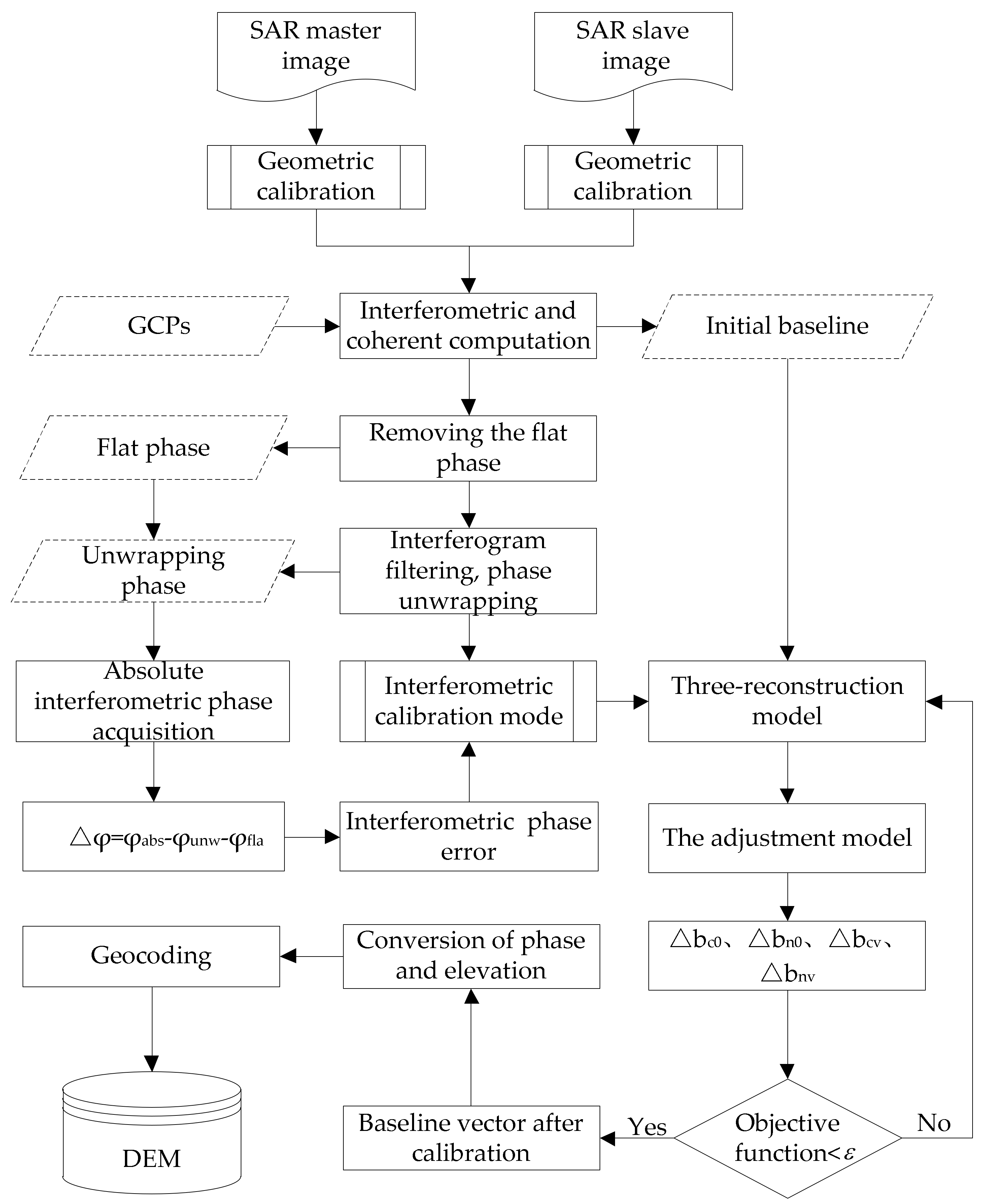
In this paper, when the baseline vector parameters are calibrated, we first start from the TDR model expression of the InSAR data; then, the sensitivity equation is established. Finally, we use the adjustment model to correct the interferometric parameters based on the least-squares criterion. To improve the accuracy of the baseline calculation, we adopt the iteration method. The root mean square error (RMSE) of the coordinate difference derived before and after the iteration is defined as the objective function. When the objective function is less than a specified threshold ($\epsilon =0.05$ in this paper), iterative convergence occurs. Finally, high-precision baseline 3D vectors are obtained to ensure the generation of high-precision DEM products. The process by which the baseline vectors are precisely estimated is shown in Figure 2 [13].

Figure 2. Methodological flow of the spaceborne SAR interferometric calibration process.

First, TDR equations representing the three coordinate axis directions are derived from the spaceborne InSAR model; these equations can be expressed as follows:

$$\left[\begin{array}{c}{F}_x\\ F_y\\ F_z\end{array}\right]=\left[\begin{array}{c}{S}_x\\ S_y\\ S_z\end{array}\right]-\left[\begin{array}{c}{P}_x\\ P_y\\ P_z\end{array}\right]+R_1\left[\begin{array}{ccc}{a}_{11}& a_{12}& a_{13}\\ a_{21}& a_{22}& a_{23}\\ a_{31}& a_{32}& a_{33}\end{array}\right]\left[\begin{array}{c}{r}_v\\ r_n\\ r_w\end{array}\right]$$

(23)

where ${\left[\begin{array}{ccc}{S}_x& S_y& S_z\end{array}\right]}^{ \mathrm{T}}$ are the coordinates of the master antenna phase center, ${\left[\begin{array}{ccc}{P}_x& P_y& P_z\end{array}\right]}^{ \mathrm{T}}$ are the coordinates of the GCP, $R_1$ is the slant range between the phase center of the master antenna and the GCP and $\left[\begin{array}{ccc}{a}_{11}& a_{12}& a_{13}^{}\\ a_{21}& a_{22}& a_{23}\\ a_{31}& a_{32}& a_{33}\end{array}\right]$ is the transformation matrix.

Second, the partial derivative of the baseline vector is calculated based on the TDR equation, and the interferometric sensitivity equation is established; this equation can be expressed as follows:

$$\left[\begin{array}{c}\frac{\partial F_x}{\partial X}\\ \frac{\partial F_y}{\partial X}\\ \frac{\partial F_z}{\partial X}\end{array}\right]=\left[\begin{array}{c}\frac{\partial S_x}{\partial X}\\ \frac{\partial S_y}{\partial X}\\ \frac{\partial S_z}{\partial X}\end{array}\right]+\frac{\partial R_1}{\partial X}\left[\begin{array}{ccc}{a}_{11}& a_{12}& a_{13}\\ a_{21}& a_{22}& a_{23}\\ a_{31}& a_{32}& a_{33}\end{array}\right]\left[\begin{array}{c}{r}_v\\ r_n\\ r_w\end{array}\right]+R_1\left\{\left[\begin{array}{ccc}\frac{\partial a_{11}}{\partial X}& \frac{\partial a_{12}}{\partial X}& \frac{\partial a_{13}}{\partial X}\\ \frac{\partial a_{21}}{\partial X}& \frac{\partial a_{22}}{\partial X}& \frac{\partial a_{23}}{\partial X}\\ \frac{\partial a_{31}}{\partial X}& \frac{\partial a_{32}}{\partial X}& \frac{\partial a_{33}}{\partial X}\end{array}\right]\right.\left[\begin{array}{c}{r}_v\\ r_n\\ r_w\end{array}\right]+\left[\begin{array}{ccc}{a}_{11}& a_{12}& a_{13}\\ a_{21}& a_{22}& a_{23}\\ a_{31}& a_{32}& a_{33}\end{array}\right]\left.\left[\begin{array}{c}\frac{\partial r_v}{\partial X}\\ \frac{\partial r_n}{\partial X}\\ \frac{\partial r_w}{\partial X}\end{array}\right]\right\}$$

(24)

The error equation is then established as follows:

$$V_B=\left[\begin{array}{cccc}\frac{\partial F_{x1}}{\partial b_{c0}}& \frac{\partial F_{x1}}{\partial b_{cv}}& \frac{\partial F_{x1}}{\partial b_{n0}}& \frac{\partial F_{x1}}{\partial b_{nv}}\\ \frac{\partial F_{y1}}{\partial b_{c0}}& \frac{\partial F_{y1}}{\partial b_{cv}}& \frac{\partial F_{y1}}{\partial b_{n0}}& \frac{\partial F_{x1}}{\partial b_{nv}}\\ \frac{\partial F_{z1}}{\partial b_{c0}}& \frac{\partial F_{z1}}{\partial b_{cv}}& \frac{\partial F_{z1}}{\partial b_{n0}}& \frac{\partial F_{x1}}{\partial b_{nv}}\\ ...& ...& ...& ...\\ \frac{\partial F_{xn}}{\partial b_{c0}}& \frac{\partial F_{xn}}{\partial b_{cv}}& \frac{\partial F_{xn}}{\partial b_{n0}}& \frac{\partial F_{xn}}{\partial b_{nv}}\\ \frac{\partial F_{yn}}{\partial b_{c0}}& \frac{\partial F_{yn}}{\partial b_{cv}}& \frac{\partial F_{yn}}{\partial b_{n0}}& \frac{\partial F_{yn}}{\partial b_{nv}}\\ \frac{\partial F_{zn}}{\partial b_{c0}}& \frac{\partial F_{zn}}{\partial b_{cv}}& \frac{\partial F_{zn}}{\partial b_{n0}}& \frac{\partial F_{zn}}{\partial b_{nv}}\end{array}\right]\left[\begin{array}{c}\Delta b_{c0}\\ \Delta b_{cv}\\ \Delta b_{n0}\\ \Delta b_{nv}\end{array}\right]+\left[\begin{array}{c}\left(F_{x1}\right)-\\ \left(F_{y1}\right)-\\ \left(F_{z1}\right)-\\ \cdots \\ \left(F_{xn}\right)-\\ \left(F_{yn}\right)-\\ \left(F_{zn}\right)-\end{array}\begin{array}{c}{F}_{x1}\\ F_{y1}\\ F_{z1}\\ \cdots \\ F_{xn}\\ F_{yn}\\ F_{zn}\end{array}\right]$$

(25)

where $\Delta b_{c0}$ and $\Delta b_{cv}$ denote the correction of the initial baseline and the baseline rate in the C direction, respectively, and $\Delta b_{n0}$ and $\Delta b_{nv}$ denote the correction of the initial baseline and the baseline rate in the N direction, respectively. The observation error can be calculated as follows:

$${\left[\begin{array}{ccc}(F_{x1})& \cdots & (F_{zn})\end{array}\right]}^{\mathrm{T}}={\left[\begin{array}{ccc}{P}_{x1}^0-P_{x1}& \cdots & P_{zn}^0-P_{zn}\end{array}\right]}^{\mathrm{T}}$$

(26)

where ${\left[\begin{array}{ccc}{P}_{xi}^0& P_{yi}^0& P_{zi}^0\end{array}\right]}^{ \mathrm{T}}$ are the three-dimensional reconstruction coordinates of the targets, ${\left[\begin{array}{ccc}{P}_{xi}^{}& P_{yi}^{}& P_{zi}^{}\end{array}\right]}^{ \mathrm{T}}$ are the coordinates of the known GCP, and ${\left[\begin{array}{ccc}{F}_{x1}& \cdots & F_{zn}\end{array}\right]}^{ \mathrm{T}}=0$ is the true observed value.

In the interferometric calibration process, the observation accuracy usually varies due to different observation conditions; thus, the introduced errors are often different. The coherence coefficient is an important criterion used to evaluate the quality of SAR images. Therefore, in this work, the coherence coefficients of the GCPs are weighted, and the objective function is expressed as follows:

$$J_{\min }=V^{\mathrm{T}}WV$$

(27)

where $W$ is the diagonal matrix. The diagonal matrix can be written as follows:

$$W=\left[\begin{array}{cccc}{w}_1& 0& \cdots & 0\\ 0& w_2& & ⋮\\ ⋮& & \ddots & 0\\ 0& \cdots & 0& w_n\end{array}\right]$$

(28)

where $w_i$ is the coherence coefficient of each GCP.

Finally, given the initial values of the baseline vector parameters, the normal equation can be established as follows:

$$A^{\mathrm{T}}WAX-A^{\mathrm{T}}WL=0$$

(29)

The baseline vector was corrected based on the normal equation, which could be denoted as follows:

$$\Delta X=(A^{\mathrm{T}}WA{)}^{-1}{A}^{\mathrm{T}}WL$$

(30)

The first estimation of the baseline vector was obtained as follows:

$$X=X_0+\Delta X$$

(31)

5. Experiments and Analyses

5.1. Experimental Data

In this work, the research areas are located in southern Nanyang city in Henan Province and in northern Xiangyang city and western Jingzhou city in Hubei Province. The whole study area covered approximately 55 km in the east–west direction and 411 km in the north–south direction. The topographic relief is very small, and the topographic type is typical flat terrain. The geographical location of the study area is shown in Figure 3. Fifty-six GCPs were acquired from the differential global positioning system (DGPS) in the geodetic coordinate system. The plane positioning error was 15 cm, and the elevation measurement error was 20 cm. The interferometric phase error was less than 1.12°, allowing these data to be used for high-precision measurement calibration tasks. Road intersections, house corners and other feature points were selected as GCPs in this paper [33], and the detailed GCP distribution is shown by the green triangles in Figure 3b,c. Before using the Ice, Cloud and Land Elevation Satellite (ICESat) data, it was necessary to filter out some data with elevation errors of tens or even hundreds of meters due to the presence of clouds, trees or buildings. In the end, a total of 10,438 points were selected, and the detailed point distribution is shown using the red dots in Figure 3b,c.

Figure 3. The study area considered in this paper: (a) the geographical location of the study area, (b) enlarged views of areas A to D, and (c) enlarged views of areas E to F. In (b,c), the white wireframes indicate the coverage of the SAR images, the green triangles denote GCPs, and the red points are the ICESat track.

We chose six FS1 GF-3 images obtained in the descending direction to conduct our interferometric calibration experiment. Table 2 presents the derived statistics on the experimental image parameters. The images are denoted as A–F from top to bottom. SAR images A, C and F were acquired on 29 November 2016, while SAR images B, D and E were acquired on 28 December 2016. In this paper, a total of four pairs of interferometric regions were formed. The number of interferometric pairs, as well as the initial baseline and baseline rates in the TCN coordinate system, are listed in Table 2. The polarization mode was HH, the incident angle was 42.8 degrees, the range resolution was 2248 m and the azimuth resolution was 2865 m. SRTM data at a 90 m grid size were selected as the external reference DEM data.

Table 2. Parameters of experimental images.

ID	Initial Baseline in the TCN Direction (m)	Baseline Rate in the TCN Direction (m/s)
A–B	0, 1087.691, 419.482	0, 0.596, 0.182
B–C	0, −1090.332, −419.650	0, −0.575, −0.070
C–D	0, 1092.000, 420.847	0, 0.723, 0.065
E–F	0, −1117.443, −423.586	0, −0.506, −0.066

5.2. Results and Analysis

5.2.1. Plane Positioning Accuracy Analysis

The plane positioning accuracies of the SAR images were evaluated using an indirect positioning algorithm (IPA). First, the image coordinates and geodetic coordinates of the GCPs were obtained. Then, the geodetic coordinates of the GCPs were transformed into image coordinates with the IPA. Finally, the RMSEs of the azimuth and range directions of all GCPs were obtained, and the RMSEs of the image points were calculated to evaluate the plane positioning accuracies of the SAR images. The results are shown in Table 3.

Table 3. Plane precisions of the test images before the geometric calibration process.

SAR Image Number	Number of GCPs	RMSE
		Azimuth (m)	Range (m)	Plane Precision (m)
A	15	44.789	28.803	53.251
B	15	40.553	28.160	49.371
C	15	21.523	21.293	30.275
D	15	19.574	21.288	28.919
E	15	30.531	17.282	35.082
F	15	24.074	16.763	29.335
Average		30.174	22.264	37.706

Table 3 shows that the average plane positioning accuracy of the six GF-3 images before the geometric calibration process was 37.706 m. The $\Delta t$ and $\Delta r$ corrections associated with the geometric parameter errors of each image were obtained after the six images were geometrically calibrated, and the initial time and slant range were both compensated for. The indirect geometric positioning algorithm was used to evaluate the plane positioning accuracies of the calibrated SAR images, and the results are listed in Table 4.

Table 4. Plane precision results of the test images after the geometric calibration process.

SAR Image Number	Geometric Parameter Correction		RMSE
	$\mathbf{\Delta }\mathit{t} \left(\mathbf{ms}\right)$	$\mathbf{\Delta }\mathit{r} \left(\mathbf{m}\right)$	Azimuth (m)	Range (m)	Plane Precision (m)
A	−3.229	−19.843	3.20	4.00	5.12
B	−3.227	−18.168	2.86	3.04	4.17
C	−3.229	−15.545	2.97	5.89	6.59
D	−2.733	−21.247	2.40	4.30	4.92
E	−3.401	−16.430	3.00	3.24	4.41
F	−4.632	−15.396	2.20	4.88	5.35
Average			2.77	4.22	5.09

From Table 4, it can be seen that the average plane accuracy of the six GF-3 images after the geometric calibration process was 5.09 m, the average positioning error of the ranges of the image points was 4.22 m (approximately 1.87 pixels) and the average positioning error of the azimuths of the image points was 2.77 m (approximately 0.96 pixels). These results show that the plane positioning accuracies of the SAR image after geometric calibration can ensure the vertical accuracy of the interferometric results in the subsequent calibration process.

5.2.2. Vertical Accuracy Analysis

The elevation information of the GCPs was calculated using the spaceborne SAR interferometric model, and the results were evaluated using the elevations of the known GCPs to obtain the vertical accuracies of the interferometric results, as shown in Table 5.

Table 5. Vertical accuracies of the interferometric results before the interferometric calibration process.

Interferometric Pair	Number of GCPs	Vertical Accuracy (m)
A–B	15	396.682
B–C	11	16.950
C–D	15	175.936
E–F	15	75.069
Average		166.159

Table 5 shows that the average elevation accuracy of the four pairs of GF-3 data was 166.159 m before the interferometric calibration process. We performed an interferometric calibration experiment on four pairs of GF-3 data. First, the phase error and baseline vector error were corrected based on IPD. Then, the absolute interferometric phase and baseline vector were compensated for. Finally, the vertical accuracy of the interferometric results was evaluated using the spaceborne SAR interferometric model; the evaluation results are listed in Table 6.

Table 6. Vertical accuracies of the interferometric results after the interferometric calibration process.

Interferometric Pair	Number of GCPs	Phase Error (°)	Interferometric Parameter Correction				Vertical Accuracy (m)
		$\mathbf{\Delta }\mathit{\phi }$	$\mathbf{\Delta }{\mathit{b}}_{\mathit{c}}{}_0$	$\mathbf{\Delta }{\mathit{b}}_{\mathit{n}}{}_0$	$\mathbf{\Delta }{\mathit{b}}_{\mathit{c}}{}_{\mathit{v}}$	$\mathbf{\Delta }{\mathit{b}}_{\mathit{n}}{}_{\mathit{v}}$
A–B	15	−137.337	−0.194	0.558	0.0113	−0.120	6.31
B–C	11	−96.657	−0.534	0.412	0.029	−0.010	2.26
C–D	15	−115.966	0.816	−0.592	−0.126	0.0041	4.45
E–F	15	−97.804	−0.127	0.535	0.0918	−0.034	3.70
Average							4.18

As shown in Table 6, the average vertical accuracy of the four pairs of GF-3 data was 4.18 m following the calibration process, and this accuracy meets the requirements for 1:50000-scale topographic mapping in flat areas. The vertical accuracies of the A–B, B–C, C–D and E–F pairs were 6.31 m, 2.26 m, 4.45 m and 3.70 m, respectively.

5.2.3. Spatiotemporal Analysis

To verify the applicability and stability of the calibration parameters characterizing the same-orbit images obtained at different imaging times, we conducted calibration compensation verification experiments. The interferometric calibration results of the A–B pair were compensated using those of the E–F pair, which had the longest imaging time difference in the same orbit. Finally, the accuracy of the verification data was evaluated; the evaluation results are listed in Table 7.

Table 7. Accuracy evaluation results of the verification scene data.

Interferometric Pair	Image Type	Interferometric Parameter Correction					Vertical Accuracy (m)
		$\mathbf{\Delta }\mathit{\phi } (°)$	$\mathbf{\Delta }{\mathit{b}}_{\mathit{c}}{}_0 \left(\mathbf{m}\right)$	$\mathbf{\Delta }{\mathit{b}}_{\mathit{n}}{}_0 \left(\mathbf{m}\right)$	$\mathbf{\Delta }{\mathit{b}}_{\mathit{c}}{}_{\mathit{v}} (\mathbf{m}/\mathbf{s})$	$\mathbf{\Delta }{\mathit{b}}_{\mathit{n}}{}_{\mathit{v}} (\mathbf{m}/\mathbf{s})$
E–F	Calibration scene	−97.804	−0.127	0.535	0.0918	−0.034	3.70
E–F	Verification scene	−137.337	−0.194	0.558	−0.0113	0.120	4.75

As Table 7 shows, when the calibration parameters were used to compensate for the verification scenes, the average vertical accuracy of the interferometric results without control points was 4.75 m; this accuracy meets the standard requirements of 1:50,000-scale topographic map mapping above grade 3 in flat areas in China (≤6 m) [34].

To analyze the influence of the spatial distribution of GCPs on the interferometric calibration results, we selected a pair of interferometric data (pair B–C) as an example and designed four schemes characterizing different spatial distributions of GCPs. In schemes (a), (b) and (c), six points were selected, while in scheme (d), 11 points were selected. The GCPs in scheme (a) were distributed along the azimuth, those in scheme (b) were distributed along the range and those in schemes (c) and (d) were randomly distributed, as shown in Figure 4. The number of calibration points included in schemes (a) and (b) were the same, but their spatial distribution modes were differentiated to verify the influence of the spatial distribution mode of the calibration points on the interferometric calibration results. Schemes (c) and (d) had the same calibration point distribution modes, characterized by random distributions, but the numbers of calibration points were differentiated to verify the influence of the number of calibration points on the interferometric calibration results.

Figure 4. Four GCP layout schemes considered herein: (a) denotes the distribution of the 6 points along the azimuth direction, (b) denotes the distribution of the 6 points along the range direction (c) and (d) denote the distribution of 6 and 11 points along the random direction, respectively. Where the blue triangles represent the GCPs.

Under the guarantee of the plane positioning accuracy of the utilized SAR images, the spatial distribution and number of GCPs directly affect the accuracy of the interferometric calibration results; these effects were explored by establishing four calibration schemes. The vertical accuracies of the interferometric results derived after calibration were evaluated according to the spaceborne SAR interferometric model; the results are listed in Table 8.

Table 8. Evaluation results of the interferometric calibration accuracies derived under 4 calibration schemes.

Scheme	$\mathbf{\Delta }\mathit{\phi } (°)$	$\mathbf{\Delta }{\mathit{b}}_{\mathit{c}}{}_0 \left(\mathbf{m}\right)$	$\mathbf{\Delta }{\mathit{b}}_{\mathit{n}}{}_0 \left(\mathbf{m}\right)$	$\mathbf{\Delta }{\mathit{b}}_{\mathit{c}}{}_{\mathit{v}} (\mathbf{m}/\mathbf{s})$	$\mathbf{\Delta }{\mathit{b}}_{\mathit{n}}{}_{\mathit{v}} (\mathbf{m}/\mathbf{s})$	Elevation Accuracy (m)
(a)	−108.232	−0.423	0.333	0.0760	−0.0442	2.513
(b)	−116.711	−0.425	0.334	0.0763	−0.0445	2.640
(c)	−96.543	−0.246	0.200	0.775	−0.572	5.584
(d)	−96.657	−0.534	0.412	0.0294	−0.0106	2.260

As shown in Table 8, when the number of calibration points was consistent, as between schemes (a) and (b), the elevation accuracy of scheme (a) was found to be better than that of scheme (b). Thus, the interferometric calibration accuracy was higher when the GCPs were distributed along the azimuth than along the range. While scheme (c) contained six GCPs and scheme (d) contained 11 GCPs, the GCPs in both schemes were randomly distributed in space; we found that the elevation accuracy of scheme (d) was better than that of scheme (c). Therefore, when GCPs are randomly distributed, the greater the number of points, the higher the interferometric calibration accuracy.

5.2.4. DEM Accuracy Analysis

We proposed a precise SAM calibration method based on GF-3 data. We decomposed the plane and elevation error sources in the spaceborne InSAR system by establishing IPD models; these factors are also the main sources of DEM product errors. In this paper, TanDEM-X DEM and ICESat data were used to evaluate the absolute elevation accuracy of the analyzed DEM after calibration, and the results are listed in Table 9.

Table 9. DEM accuracy evaluation results (unit: m).

Interferometric Pair	TanDEM-X DEM	ICESat
A–B	2.10	2.63
B–C	2.73	2.78
C–D	2.40	3.09
E–F	1.44	2.55

Focusing on interferometric pair A–B, following the calibration process, the absolute elevation accuracies of the derived DEM were better than 2.10 m when the TanDEM-X DEM was used and 2.63 m when ICESat data were used. Regarding interferometric pair B–C, the post calibration absolute elevation accuracies of the DEMs were better than 2.73 m when the TanDEM-X DEM was used and 2.78 m when the ICESat DEM was used. For interferometric pair C–D, the post calibration absolute elevation accuracies were better than 2.40 m when TanDEM-X DEM was applied and better than 3.09 m when ICESat was applied. Focusing on interferometric pair E–F, the absolute elevation accuracies of the calibrated DEM were better than 1.44 m when TanDEM-X DEM was used and better than 2.55 m when ICESat data were used.

To quantitatively analyze the elevation variations in the GF-3-derived DEM following the calibration process, we drew a transect in the flat area shown in Figure 5a,b according to the distribution of ICESat points. As shown in Figure 5a, this transect covers pairs A–B, B–C and C–D from the northwest to the southeast corners of the image, with a length of approximately 106 km. As shown by the black line (labeled $n$) in the figure, the section map corresponds to Figure 6a. The section line shown in Figure 5b spans from the north to the south regions of the image with a length of approximately 45 km. As shown by the black line (labeled $m$) in the figure, the section map corresponds to Figure 6b, and the elevation data of the GF-3 DEM, ICESat DEM and TanDEM-X DEM are represented by green, red and blue lines, respectively, in the figure.

Figure 5. DEM products obtained after the calibration process: (a) the DEM results corresponding to interferometric pairs A–B, B–C and C–D and (b) DEM results corresponding to interferometric pair E–F. In (a,b), the green triangles show the GCPs and the red points show the ICESat laser points.

Figure 6. Elevation distribution maps of transects m and n: (a) the elevation change along section line m in interferometric pairs A–B, B–C and C–D; (b) the elevation change along section line n in interferometric pair E–F; (c) the coherence distribution maps of interferometric pair B–C; (d) the coherence distribution results of section line m. Panels (a1–a3) and (b1,b2) contain enlarged images of regions with abnormal ICEsat points; the labels P_a1–P_b5 represent abnormal ICEsat points.

It is obvious that the elevation data contained in the GF-3 DEM and TanDEM-X DEM are basically consistent at interferometric pairs A–B, C–D and E–F. However, the elevations at some ICESat laser points are abnormal, as shown in Figure 6a1–a3,b1,b2. The information in the figure shows that the ICESat laser points in these areas are mainly distributed in building construction areas and vegetation-covered areas, possibly leading to poor elevation results. Therefore, the accuracy of the monitored GF-3 DEM products derived by comparison to the TanDEM-X DEM in this area was higher than that of the ICESat DEM.

Regarding interferometric pair B–C, the elevations of the ICESat DEM and TanDEM-X DEM were basically consistent. However, compared to the elevations of the ICESat DEM and TanDEM-X DEM, some of the elevation data in the GF-3 DEM were obviously abnormal. For further analysis, the coherence distribution was calculated in this area, as shown in Figure 6c; the coherence distribution corresponding to transect $m$ is shown in Figure 6d. According to the statistical results, the coherence of transect m was lower than 0.6, accounting for 26.5%. In other words, 26.5% of the points in this region were located in incoherent areas, mainly due to the abundant ground feature information, including water areas, vegetation areas, and residential and urban areas; this ground feature information is often the main factor leading to incoherence in satellite images. Moreover, large shadows and overlaps are generated in side-looking radar imaging, which may lead to the poor accuracy of the elevation data reflected in the GF-3 DEM obtained in these areas.

6. Conclusions

In this paper, we proposed an IPD method to support the application of SAM approaches using GF-3 SAR data. In the proposed IPD method, geometric and interferometric calibration models are separately utilized to prevent parameter coupling phenomena from arising. We decomposed the sources of geometric and interferometric parameter errors in the GF-3 SAR system by establishing IPD models, and the derived errors could also be considered the main factors affecting the resulting DEM products. Herein, the plane positioning accuracies of the SAR images, the vertical accuracies of the interferometric results and the spatiotemporal distribution characteristics and elevation accuracies of DEM products were analyzed. The correctness, reliability and practicability of the proposed method were verified. The results show that the average plane positioning accuracy of the SAR images was 5.09 m following the geometric calibration process, and the average post-calibration vertical accuracy of the interferometric results was 4.18 m. The corresponding average absolute elevation accuracy of the DEM products was better than 3.09 m. These results confirm that the method proposed herein can improve the elevation accuracies of Gaofen-3 DEM products, which met the 1:50000-scale topographic map SAM precision, or even higher precisions, in the flat areas of China. Moreover, there are still some problems to be further studied in this paper. Due to the lack of high-precision CRs, the method proposed cannot fully verify the on-orbit calibration of satellites. Follow-up research will mainly focus on this aspect.

The follow-up satellites to GF-3, i.e., the 1 m C-SAR 01 and 02, were launched on 23 November 2021 and on 7 April 2022. This ocean-monitoring SAR satellite constellation consists of three satellites. The 1 m C-SAR satellites were designed in consideration of their interferometric capabilities. An increasing number of interferograms can be provided by this new satellite constellation, and these novel interferometric data can also be obtained more easily. We hope that the proposed method will be useful in supporting the usage of these new satellites.