Estimation of Aboveground Carbon Density of Forests Using Deep Learning and Multisource Remote Sensing

Abstract

Forests are crucial in carbon sequestration and oxygen release. An accurate assessment of forest carbon storage is meaningful for Chinese cities to achieve carbon peak and carbon neutrality. For an accurate estimation of regional-scale forest aboveground carbon density, this study applied a Sentinel-2 multispectral instrument (MSI), Advanced Land Observing Satellite 2 (ALOS-2) L-band, and Sentinel-1 C-band synthetic aperture radar (SAR) to estimate and map the forest carbon density. Considering the forest field-inventory data of eastern China from 2018 as an experimental sample, we explored the potential of the deep-learning algorithms convolutional neural network (CNN) and Keras. The results showed that vegetation indices from Sentinel-2, backscatter and texture characters from ALOS-2, and coherence from Sentinel-1 were principal contributors to the forest carbon-density estimation. Furthermore, the CNN model was found to perform better than traditional models. Results of forest carbon-density estimation validated the improvements effectively by combining the optical and radar data. Compared with traditional regression methods, deep learning has a higher potential for accurately estimating forest carbon density using multisource remote-sensing data.

1. Introduction

The subtropical-forest coverage rate of Zhejiang Province reaches 61.17%, ranking among the top five in China [1], and it is crucial in regional carbon cycles and ecosystems. The area has a subtropical monsoon climate, which is suitable for the growth of forest vegetation. Accordingly, the assessment of forest aboveground carbon storage in the region is essential to learn the carbon cycle, mitigate global warming, and scientifically manage the abundant forest resources [2].

As forests account for a major part of terrestrial ecosystems, they regulate the regional ecological environment [3] and provide the largest proportion of water in all land uses [4]. The carbon-sequestration capacity of forests accounts for 76–98% of the entire terrestrial ecosystem [5] and is vital for reducing global warming caused by carbon dioxide concentration [6]. According to Sixth Assessment Report (AR6) of Intergovernmental Panel on Climate Change (IPCC), the temperature of the Earth has already increased by 1.2 °C compared to the average in 1850–1900 [7]. Under such severe conditions, increasing forest carbon storage is an effective and low-cost method to deal with global warming. As forests are the largest terrestrial carbon pool, any increase or decrease in forest carbon storage may cause changes in the global atmospheric CO₂. Thus, increasing forest carbon storage can significantly contribute to maintaining global carbon balance and mitigating climate change [8,9], and is a rapid, accurate, and macro-scale method to understand forest spatial distribution and carbon storage.

The estimation of forest carbon storage primarily includes the biomass-plot-inventory, carbon-flux-detection, and stable-isotope methods. However, the most common method is based on forest biomass calculation, which measures the production and biomass of forest vegetation directly or indirectly, and then multiplies the percentage of carbon content of the corresponding tree species [10]. This method is easy to operate, has high precision, and is extensively used; therefore, the determination of aboveground biomass is the vital parameter to estimate forest carbon storage.

Remote-sensing data are cost-effective and spatiotemporally comparable, which has been used in researching forest aboveground biomass (AGB) [11]. Combining multispectral instrument (MSI) imagery with synthetic aperture radar (SAR) can improve estimation accuracy [12]. Optical images provide abundant canopy spectral and textural information, and frequently used variables from optical sensors for estimating forest parameters include band information, vegetation indices, texture features, etc. Additional information can be obtained through image conversions such as principal component analysis and tasseled cap transformation [13]. Common predictors from radar data include backscatter coefficient, interference coefficient, texture characteristics, etc. SAR has a certain penetration depth of forest vegetation, which increases with wavelength and reflects the vertical information of forest [14]. Interferometric Synthetic Aperture Radar (InSAR) techniques are increasingly being used for earth observations [15,16,17] and can provide forest height information [18] in forest parameter inversion, and AGB is obtained indirectly using tree height substitution into the growth equation [19]. The use of multiple variables and techniques in estimating forest AGB reduces errors in forest inversion [20]. Sentinel-2 is equipped with a new multispectral imager with high spatial resolution, and contains three red-edge bands, which are used to detect the distribution and parameter inversion of forest resources. The Sentinel-1 C-band SAR acquires images under all light and weather conditions and has served with forest vegetation research [21]. The ALOS-2 L-band SAR has a better penetration of branches and leaves than the C-band and has greater potential for forest-resource monitoring [22,23]. Thus, different remote sensing data have contributed significantly to forest-resource management and research [24].

Currently, multiple linear regression is often used to estimate forest AGB, but this method cannot effectively represent nonlinear relationships, and does not always capture the relationship between the observable and AGB [25]. Therefore, machine learning is used to improve estimation accuracy [26]. In [27], three classical machine-learning approaches (multiple linear regression, support-vector regression, and random forest) were selected to predict forest parameters from Sentinel-1 data, which showed that support-vector regression and random-forest methods had better performance over the parametric multiple linear-regression method. Machine learning involves the selection of parameters that are related to unclear physical mechanisms. Owing to the complex spatial heterogeneity and dynamic changes in forest ecosystems, studies on remote-sensing predictors, model construction, and accuracy of forest AGB estimation continue to face many challenges. Deep-learning (DL) algorithms have been developed to identify complex nonlinear relationships in data [28]. Ref. [29] proposed and evaluated the use of deep-learning-based methods and unmanned aerial-vehicle-based RGB images to estimate the value of biomass yield in the models, which were able to establish a high correlation between the images and the biomass value measured in the field. DL models can use multiple successive hidden layers, and the learning process involves determining the parameter values of each layer. In recent years, various geospatial analytic projects have used DL algorithms [30,31]. A study [32] proposed a deep-learning-based water-body-extraction model that exploited sentinel-1 data and flood-related geospatial datasets. Through validation, the DL model improved the accuracy of image water-body extraction by 7.68 percent. DL has been extensively studied with image processing and classification; however, few studies have been conducted on its application in estimating forest carbon storage and AGB, particularly using the different models and types of DL. In this study, Keras and convolutional neural network (CNN) methods were used to calculate forest AGB, and the results were compared with those of other methods.

The purpose of this study was to (1) use different satellite data to explore the relationship of different variables and their combinations with AGB and carbon storage of subtropical forests in China; (2) compare different regression-learning models to analyze whether DL methods could increase the accuracy of forest AGB; and (3) develop a carbon-storage map for the study region to support spatial analysis and forest-resource management.

This paper includes five sections. Section 2 presents information on the characteristics of the study area, climate, ground data, and remote-sensing data, and also describes the principles of five experimental methods for estimating forest AGB. Section 3 shows the results. Section 4 is a discussion, and finally Section 5 provides the main conclusions of the article.

2. Materials and Methods

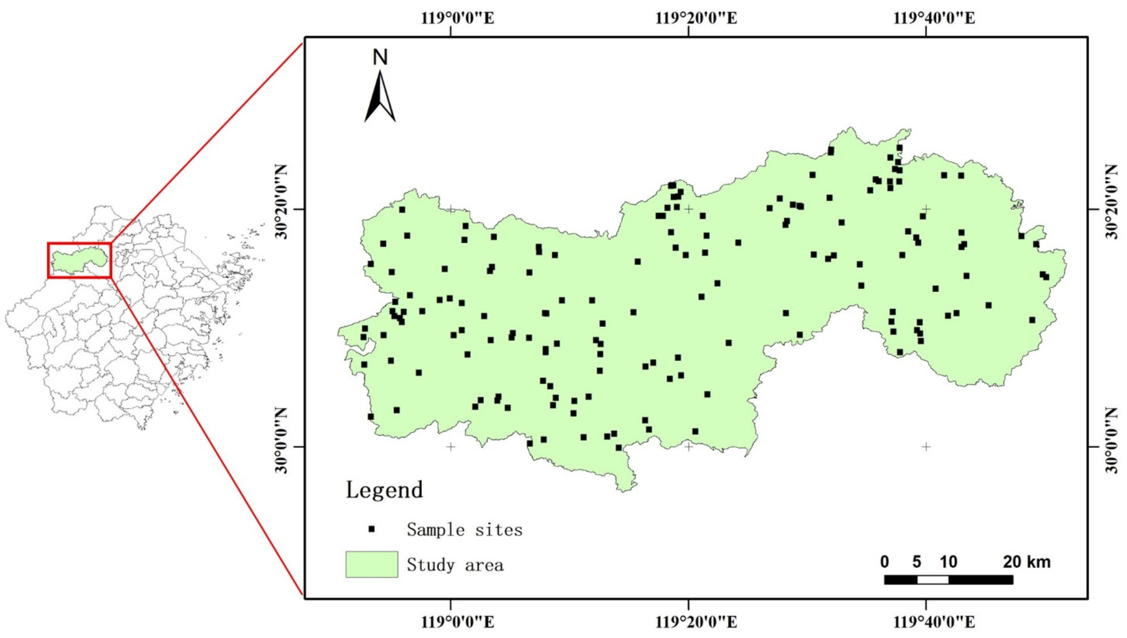
2.1. Description of Study Area

Lin’an district (118°51′–119°52′E, 29°56′–30°23′N), Hangzhou City, Zhejiang Province in eastern China was chosen as the study area of this study (Figure 1). Zhejiang Province has a subtropical monsoon climate, with an average annual temperature of 16.4 °C and 1500.0–1628.6 mm of precipitation. The region is sparsely covered by hills with a high forest-coverage rate and high species richness. The dominant species are Pinus massoniana and Cunninghamia lanceolate, and the main forest types include coniferous mixed and broadleaf mixed forests.

2.2. Data Collection and Processing

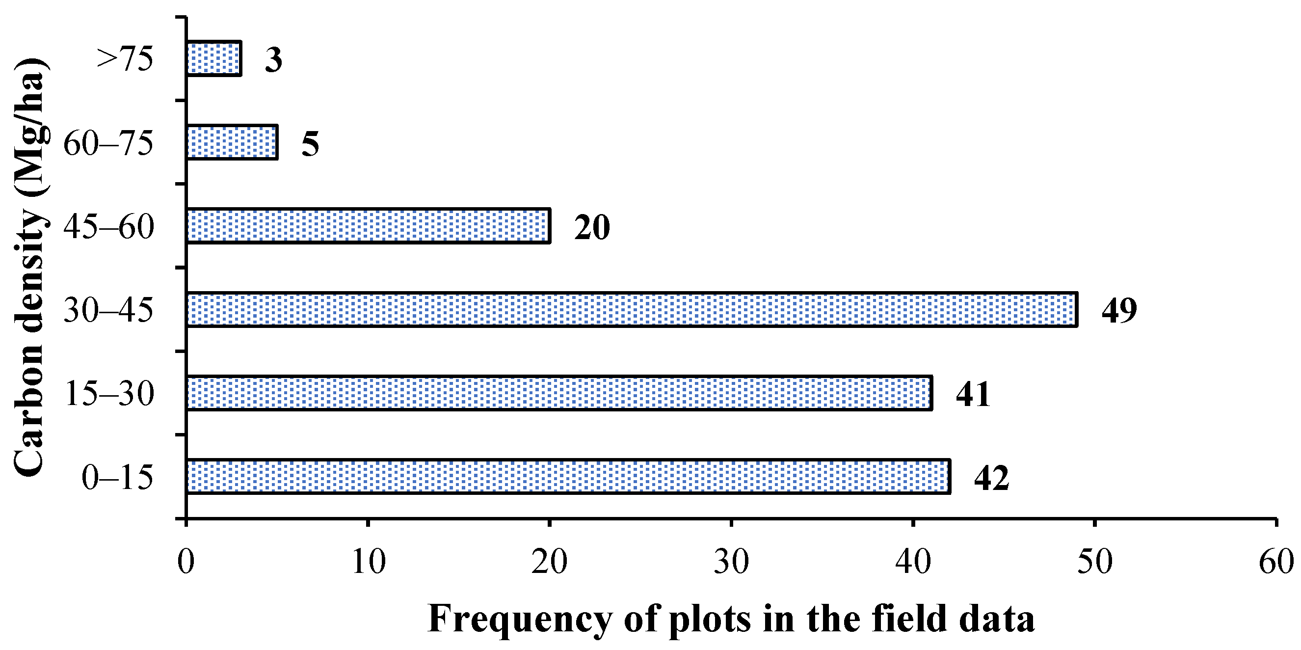
2.2.1. Field Data

The goal of a national forest-resource continuous inventory is to acquire the quantity, quality, growth, and extinction patterns of forest resources. This is a significant component of the comprehensive detection of environmental conditions and forest resources in China. Forest inventory data are the most systematic, comprehensive, and accurate data that reflect the status of forest resources, and include forest types, stock, growth, and harvesting [33].

The ground data of this study were obtained from the ninth forest-resource inventory in 2018. The data included 160 forested plots covering an area of 0.067 hectare (ha). The data comprised the location, date of measurement, origin, and forest species composition of the plots. For each plot, the main investigation parameters were tree species, tree age, tree height, and diameter at breast height (DBH).

Forest AGB were calculated using DBH and tree height, which were from field studies at different sampling sites. Based on the growth models and parameters of various tree species or tree groups reported in literature, the AGB of individual living trees was estimated for each tree species (

Table 1. Allometric growth equations of major tree species in the study region, where W is the AGB, D is the DBH, and H is the tree height.

Tree Species	Model Expression and the Parameters
Cunninghamia lanceolata group	W = 0.0492Power(D, 2.660)
Pinus massoniana group	W = 0.1309Power(D, 2.4367)
Hard broadleaf group	W = 0.0710Power(D2H, 0.9117)
Soft broadleaf group	W = 0.1351Power(D2H, 0.8020)

). According to the forest distribution statistics of the study area, the dominant tree species were divided into four types: Cunninghamia lanceolata, Pinus massoniana, hard broad leaves, and soft broad leaves. After calculating the forest AGB, the carbon storage of a certain tree species (forest type) was obtained by multiplying the AGB by the carbon content [34]. In numerous forest carbon-storage estimation studies, the internationally commonly used tree carbon-content rates such as 0.45 [35], 0.5 [36], or 0.55 [37] are usually used to convert forest AGB to carbon storage. In this paper, the carbon-content rate of the main dominant tree species in the study area is 0.5 [38], so the conversion coefficient of this study was set at 0.5 [3,39]. The carbon storage of aboveground parts of each tree was directly converted from the estimated AGB of the tree. The carbon storage was calculated as follows:

$$C=W\times CF$$

(1)

where C is the carbon storage, W is the forest AGB, and CF is the carbon content.

The carbon density of the quadrats and the number of related stands were obtained according to the conversion relationship (Figure 2). Most of the quadrats exhibited carbon density at 30–45 Mg/ha with fewer quadrats having high (>60 Mg/ha) carbon density.

2.2.2. Optical and Radar Data Processing

We used optical (Sentinel-2) and radar (ALOS-2 PALSAR-2 and Sentinel-1) remote-sensing data.

Based on the ground survey time and the location of the study area, two Sentinel-2 Level-1C multispectral optical images with good imaging quality were downloaded. The imaging times were 29 October and 10 November 2018, which were consistent with the field-investigation times. The atmospheric-correction processor SEN2COR was used for atmospheric correction, which was based on the radiative-transfer model. Installing the SEN2COR plugin in SNAP software (version 8.0, European Space Agency, Paris, France) and level-2A products were obtained [40]. After cropping and mosaicking the Sentinel-2 images, eight texture features were acquired using a gray-level co-occurrence matrix (GLCM) with a window size of 5 × 5.

We used data from two synthetic-aperture radar satellites: the ALOS-2 PALSAR-2 L-band SAR data from the Japan Aerospace Exploration Agency and Sentinel-1 C-band data of the European Aviation Agency. Four ALOS-2 single-look complex (SLC) images for 8 November 2018, were captured in fine-beam double-polarization (FBD) mode at a Level-1.1. In addition, we downloaded two images of C-band Sentinel-1A Level-1 IW SLC products from Copernicus Sentinel Scientific Data Hub on 1 October and 13 October 2018. The procedures were completed using SNAP software, combined with 30 m spatial resolution DEM data. The processing of ALOS-2 data consisted of the following steps: radiometric correction, coherent speckle filtering by Lee filter to suppress speckle and noise, with a window size of 5 × 5, and terrain correction by Range–Doppler method. Sentinel-1 data were subject to orbit correction in addition to the above steps [41]. Then, the backscatter intensity was normalized by radiometric calibration to obtain the backscatter coefficient in decibels. In addition, the SNAP toolbox was applied to Sentinel-1 image processing by coherent interference; the main procedures included co-registration, interferogram formation, topographic-phase removal, phase filtering by Goldstein phase filtering, and terrain correction by Range–Doppler method. The acquisition data and basic information of the remote-sensing data used in the paper are shown in

Table 2. The remote-sensing data sources used in study area.

Data Sources	Acquisition Data	Processing Level	Spectral/Polarization Used
Sentinel-2	29 October 2018 10 November 2018	Level-1C	10 multispectral bands
Sentinel-1	1 October 2018 13 October 2018	Level-1 IW SLC	C-band, VV and VH polarizations
ALOS-2 PALSAR-2	25 October 2018 8 November 2018	Level 1.1	L-band, HH and HV polarizations

Note: VV, transmitting and receiving both with vertical polarization; VH, transmitting with vertical polarization and receiving with horizontal polarization; HH, transmitting and receiving both with horizontal polarization; HV, transmitting with horizontal polarization and receiving with vertical polarization.

.

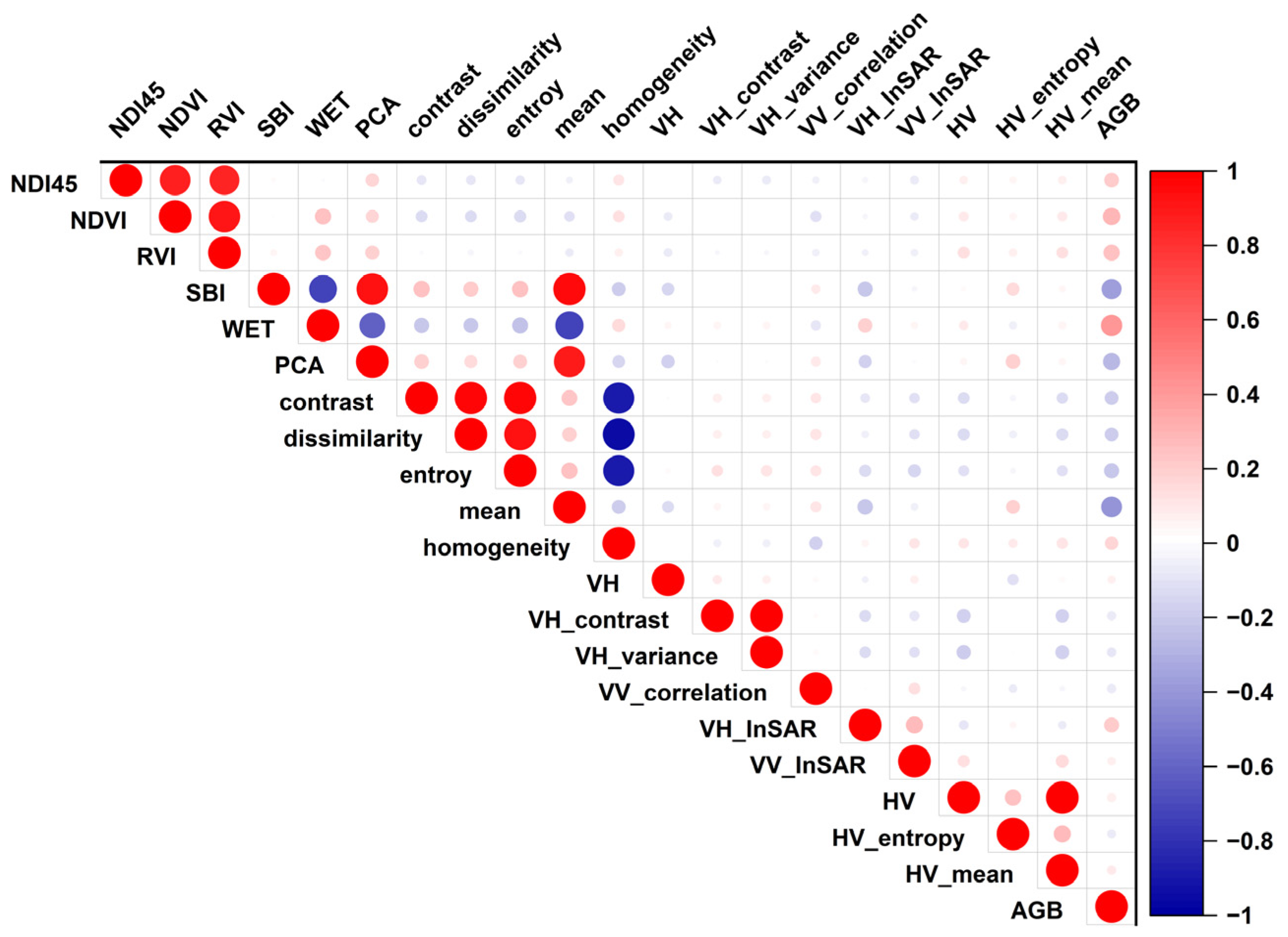
2.3. Characteristic Variables Selection

We selected and calculated 67 variables, and 29 variables were derived from Sentinel-2 images, including band reflectance (excluding three atmospheric bands 1, 9, and 10), vegetation index, texture feature, tassel-cap transform factor, and principal-component-analysis factor. In addition, 20 variables of VV, VH backscattering coefficient, texture features, and coherence were extracted from the Sentinel-1 images. Based on the ALOS-2 images, 18 variables were extracted, including HH, HV backscattering coefficients, and texture feature parameters (

Table 3. Description of different indices from remote-sensing data.

Data	Characteristic Type	Indices	Description
Sentinel-2	Bands	B2, 3, 4, 5, 6, 7, 8, 8a, 11, and 12	Three “atmospheric” bands B1, 9, and 10 were removed
	Vegetation indices	NDVI	Normalized difference vegetation index, NDVI = (B8 − B4)/(B8 + B4)
		DVI	Difference vegetation index, DVI = B8 − B4
		GNDVI	Green normalized difference vegetation index, GNDVI = (B7 − B3)/(B7 + B3)
		NDI45	Normalized difference vegetation index with band 4 and 5,NDI45 = (B5 − B4)/(B5 + B4)
		REIP	Red-edge infection point index, REIP = 700 + (40 × ((B4 + B7)/2 − B5))/(B6 − B5)
		RVI	Ratio vegetation index, RVI = B8/B4
		S2REP	Sentinel-2 red-edge position index, S2REP = 705 + (35 × ((B4 + B7)/2 − B5))/(B6 − B5)
	Biophysical variables	SBI	Tasseled cap transformation, SBI = 0.3037 × B2 + 0.2793 × B3 + 0.4743 × B4 + 0.5585 × B8 + 0.5082 × B11 + 0.1863 × B2
		GVI	GVI = −0.2848 × B2 − 0.2435 × B3 − 0.5436 × B4 + 0.7243 × B8 + 0.084 × B11 − 0.18 × B12
		WET	WET = 0.1509 × B2 + 0.1973 × B3 + 0.3279 × B4 + 0.3406 × B8 − 0.7112 × B11 − 0.4572 × B12
		PCA	Principal component analysis
	Texture	Mean, variance, contrast, dissimilarity, homogeneity	8 texture features extracted Texture by GLCM of 5 × 5 window size
ALOS-2	Backscatter coefficients	HH_db, HV_db	Backscatter coefficient of the horizontal transmit-horizontal and transmit-vertical receive channel in dB
	Texture	HH or HV_Contrast	Contrast, local variations
		HH or HV_Dissimilarity	Dissimilarity, degree of similarity
		HH or HV_Homogeneity	Homogeneity, uniformity of color tone
		HH or HV_Angular second moment	Angular second moment, degree of order of texture distribution
		HH or HV_Mean	Mean, average of grayscale values
		HH or HV_Variance	Variance, change of grayscale values
		HH or HV_Correlation	Correlation, linear correlation between the image elements
		HH or HV_Entropy	Entropy, disorder of texture distribution
Sentinel-1	Backscatter coefficients	VV_db, VH_db	Backscatter coefficient of the vertical transmit-vertical and transmit-horizontal receive channel in dB
	Texture	VV or VH_Contrast, VV or VH_Dissimilarity, VV or VH_Homogeneity, VV or VH_Angular second moment, VV or VH_Mean, VV or VH_Variance, VV or VH_Correlation, VV or VH_ ntropy	The texture feature of VV and VH. Same as mentioned above
	InSAR	VV_InSAR, VH_InSAR	Interference coherence of VV and VH

).

2.4. Experimental Models

Remote-sensing predictor variables and forest AGB have a nonlinear relationship, and the AGB is commonly estimated in a data-driven manner by using nonlinear models. Experiments are necessary to determine the most suitable machine-learning algorithm. A comparison of different algorithms can discover the complex nonlinear relationship. Therefore, this study used multiple linear regression (MLR) analysis, support-vector machine (SVM), random forest (RF), and DL (including Keras and CNN) to predict the AGB regression.

2.4.1. Multiple Linear Regression

MLR is a regression-analysis method that applies multiple independent variables to estimate unknown variables to describe the linear relationship between independent and dependent variables [42,43]. In this study, MLR was applied to establish a linear function between the measured AGB and the information parameters, and then estimated the AGB using the model without the requirement of measured data. The model is relatively simple and easy to understand and does not require highly processed remote-sensing data [44]; therefore, it is widely used in forest AGB estimation. The model is mathematically represented as follows.

$$\mathrm{y}=b_0+b_1{x}_1+b_2{x}_2+\cdots +b_n{x}_n+\epsilon$$

(2)

where y is the predicted forest AGB, $x_1\cdots x_n$ are the information parameters, $\epsilon$ is the error term, $b_0$ is a constant, and $b_1\cdots b_n$ are the regression coefficients.

2.4.2. Support Vector Machine

No assumption is required of the SVM model for the underlying data distribution and dimensions of the input space and provides a group of classified data samples [24]. In addition, SVM is applied to regression, which is known as support-vector regression (SVR). Numerous existing studies have applied SVR to remote-sensing quantitative estimation, such as ocean chlorophyll-concentration inversion [45], biomass estimation [46], etc.

In this study, we adopted an SVR algorithm based on MATLAB (The MathWorks, Inc., Natick, MA, USA) and selected a radial-basis kernel function. SVR optimization is primarily based on c and g [47], which are the most important components of SVM; c is the penalty coefficient, which refers to the error tolerance range; and g is the internal parameter of the kernel function used to determine the distribution of the data after mapping to the new feature space. Parameter settings of SVR algorithms are quite important. Therefore, c and g were tested within certain value intervals for each characteristic set for the algorithm to determine the most accurate value.

2.4.3. Random Forest

RF consists of multiple decision trees selected according to certain conditions to achieve a goal, and is used for classification and regression prediction [48,49]. The bootstrap-sampling method was applied in this study to conduct random sampling with replacement of the samples. Each sampling result was used to construct a regression tree, and multiple decision trees were combined to form an RF model. The variables were screened and classified using the model to predict the unknown parameters. RF does not require the assumption of a prior probability distribution; therefore, it has good flexibility and stability, as well as high computation speed and accuracy [14].

We used TreeBagger in MATLAB to implement the RF model construction. The number of decision trees (n) and the number of variables preselected by the tree nodes (m) were two important parameters that must be determined in the algorithm. The results were determined through multiple iterations; m was set to 5 and n to 500, and the error was stable.

2.4.4. Keras

TensorFlow (Google Inc., Menlo Park, CA, USA) is the most extensively used and popular low-level framework [30]. Keras is a well-known advanced DL framework with TensorFlow as its backend engine [50]. Keras was written in Python in this study, and the sample data were randomly split into a training part and a testing part. Three hidden layers were added to the model. The first two were set with eight neurons, and the last one with one neuron, and a rectified linear unit (ReLU) was selected as the activation function. The loss function was used as an index to measure the learning performance, which was set as the mean-square error in this regression problem. Adaptive-moment estimation (Adam) was set the weights of different neural corrections as the optimization function [51]. An early stop function was set to prevent the model from overfitting, and 50 as a patience value, implying that the loop automatically ends if the accuracy does not improve after 50 operations.

2.4.5. Convolutional Neural Network

The CNN algorithm reduces the processing of a large number of parameters by sharing a convolution kernel within each layer, and the convolution algorithm can improve high-level abstract features from spatial information [52]. The specific equation is as follows:

$$ma{p}_{l,j}^{x,y}=f\left({\displaystyle \sum }_{\delta }{\displaystyle \sum }_{h=0}^{h_i-1}{\displaystyle \sum }_{w=0}^{w_i-1}{k}_{i,j,\delta }^{h,w}ma{p}_{\left(i-1\right),\delta }^{\left(x+h\right),\left(y+w\right)}+b_{i,j}\right)$$

(3)

where f(x) is an activation function; $k_{l,j,\delta }^{h,w}$ are the values of the kernel at the position (h, w) associated to the $\delta$th feature map in the (i − 1)th layer; $h_i$ are the height of the kernel;$w_i$ are the width of the kernel; and $b_{i,j}$ is the bias of the jth feature map in the ith layer.

In the process of backpropagation, the derivative is propagated back along the calculated path, and the derivative of the loss for each parameter is calculated according to the chain derivative equation [53]. The Adam algorithm was used for optimization [54]. The Adam optimizer combines momentum and adaptive learning rate with the advantages of stable optimization, and the adaptive learning rate does not easily fall into the local optima. The iterative equations for the Adam algorithm are as follows:

$$Y_1={\alpha }_1\times Y_1+\left(1-{\alpha }_1\right)\times gra{d}_w$$

(4)

$$Y_2={\alpha }_2\times Y_2+\left(1-{\alpha }_2\right)\times {\left(gra{d}_w\right)}^2$$

(5)

$$b_1=\frac{Y_1}{1-{\alpha }_1^t}$$

(6)

$$b_2=\frac{Y_2}{1-{\alpha }_2^t}$$

(7)

$$\omega =\omega -b_1\times \frac{l_r}{\sqrt{b_2}+\theta }$$

(8)

where $gra{d}_w$ is the influence of parameter w in each neural network on the best loss; $Y_1$ and $Y_2$ are the first and second momenta, respectively; $b_1$ and $b_2$ are the $Y_1$ and $Y_2$ adjustments to prevent a longer step at the start of the training; ${\alpha }_1$ and ${\alpha }_2$ are the rates of the momentum decrease; t is the number of training epochs; $l_r$ is the learning rate; and $\theta$ is used to avoid the error of dividing by 0.

We adopted a simplified CNN structure to facilitate multiple repetitions, reduce the impact of the samples, and experiment the input-window size. The CNN included two fully connected layers with a window size of 3 × 3. The Adam algorithm was used for optimization, the activation function was ReLU, and the loss function was the root-mean-square error (RMSE).

2.5. Model Accuracy Evaluation

The RMSE and determinant coefficient (R²) were chosen as model evaluation parameters to compare the depth-regression model with the other models [55]. The R² range is [0, 1]; generally, the closer it is to 1, the better the model performance. Because the number of observations (n) is limited in practical applications, the RMSE can better reflect the maximum and minimum errors of a set of data and reflect the precision of the data estimation. As a rule, the model that has a high R² and a low RMSE fits well with the sample, and the model exhibits good performance.

$$\mathrm{RMSE}=\sqrt{\frac{1}{n}{\displaystyle \sum }_{i=1}^n{\left(Y_i-{\widehat{Y}}_i\right)}^2}$$

(9)

$${\mathrm{R}}^2=1-\frac{{{\displaystyle \sum }}_{i=1}^n{\left(Y_i-{\widehat{Y}}_i\right)}^2}{{{\displaystyle \sum }}_{i=1}^n{\left(Y_i-{\overline{Y}}_i\right)}^2}$$

(10)

where Y_i is the measured forest AGB, ${\widehat{Y}}_i$ is the calculated forest AGB by models, and ${\overline{Y}}_i$ is the average observer forest AGB.

3. Results

3.1. Predicted Variables

According to SPSS (version 24.0, IBM, Armonk, NY, USA) experiment of Pearson’s product-moment correlation, feature parameters with significant correlations were selected, r values indicted the relationship between predictors and AGB. For the analysis, if all relevant feature parameters were included in the model, the results would not be ideal [56]. Therefore, referring to existing research [57], information redundancy between the predictors produces a large error, which occurs between model building and forecasting, and by understanding each factor’s physical significance, we screened the variables and eliminated the predictors with weak correlation with AGB in the same category of redundant parameters. The 20 variables with high correlation coefficients with forest AGB are shown in Figure 3, which also demonstrates the correlation coefficients between the variables. Finally, 11 predicted variables for estimating forest AGB were obtained (

Table 4. Selected predictors derived from remote-sensing data and correlation coefficient with AGB (“**” denotes that the p < 0.01).

Data	Characteristic Type	Predictor Variables	r
Sentinel-2	Vegetation indices	NDVI	0.282 **
	Biophysical variables	WET	0.420 **
		SBI	−0.368 **
	Texture	Mean	−0.405 **
Sentinel-1	Backscatter	VH_db	0.072 **
	Interference coherence	VH_InSAR	0.212 **
	Texture	VH_Contrast	−0.079 **
		VH_Variance	−0.083 **
ALOS-2	Backscatter	HV_db	0.079 **
	Texture	HV_Mean	0.082 **
		HV_Entropy	−0.077 **

).

3.2. Model Test Results

3.2.1. MLR Model

To discover the quantitative relationships between multiple variables, regression analysis is used in this study. According to the correlation-analysis experiments of the independent variables and AGB of the sample plots, 11 characteristic variables were extracted from different data sources in SPSS, and the MLR model was constructed based on different data sources. Figure 4 showed the obtained regression models and their accuracies.

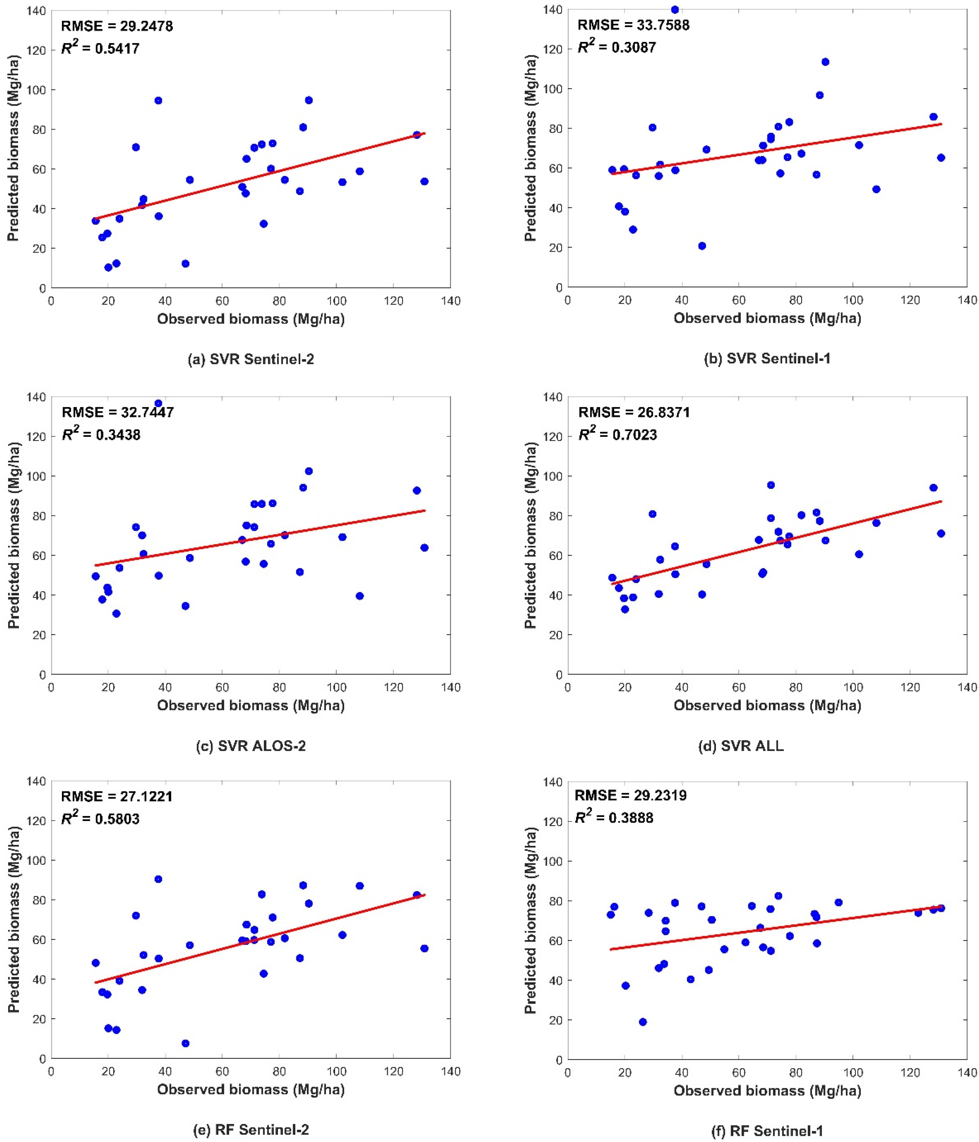
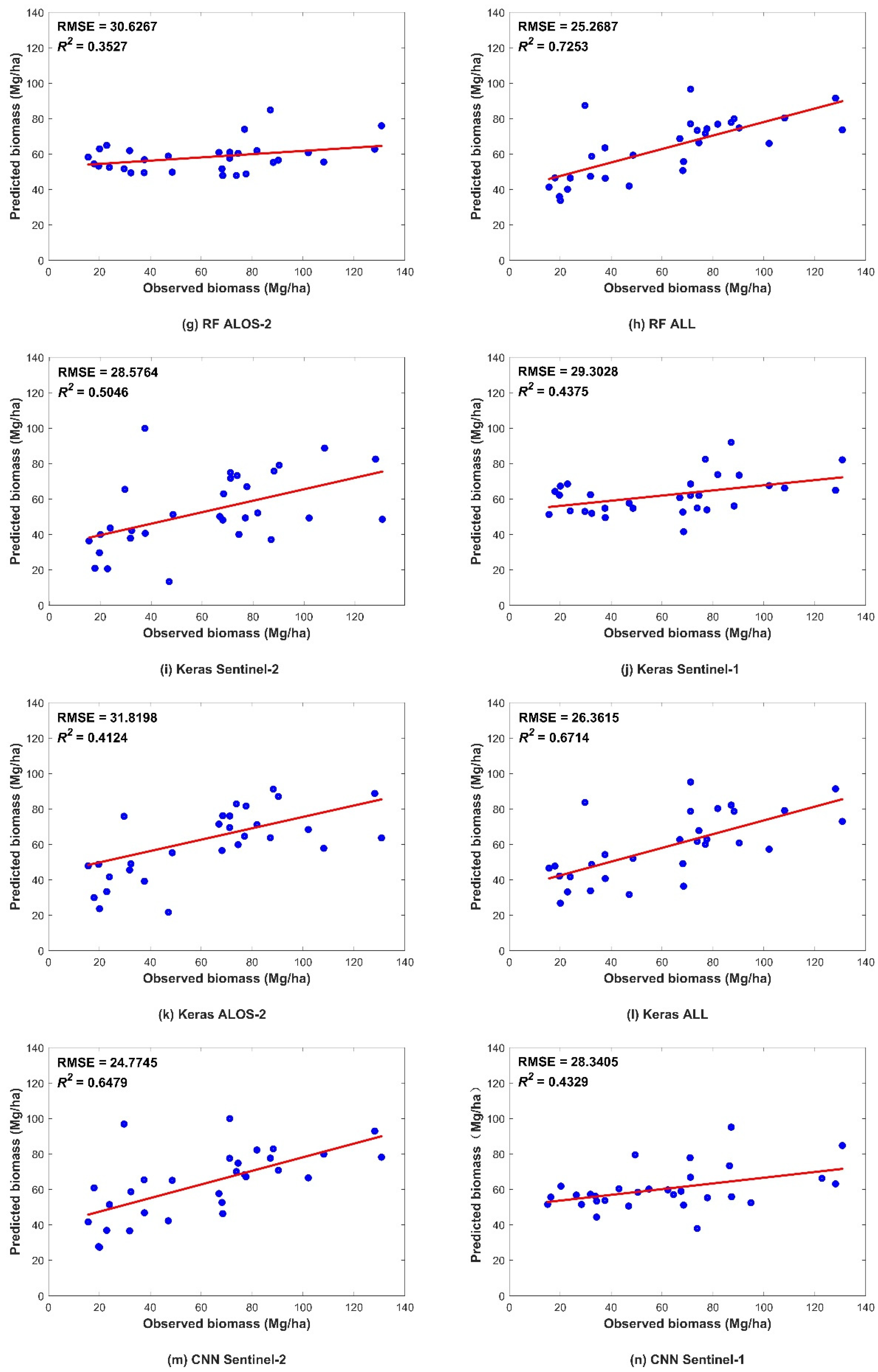
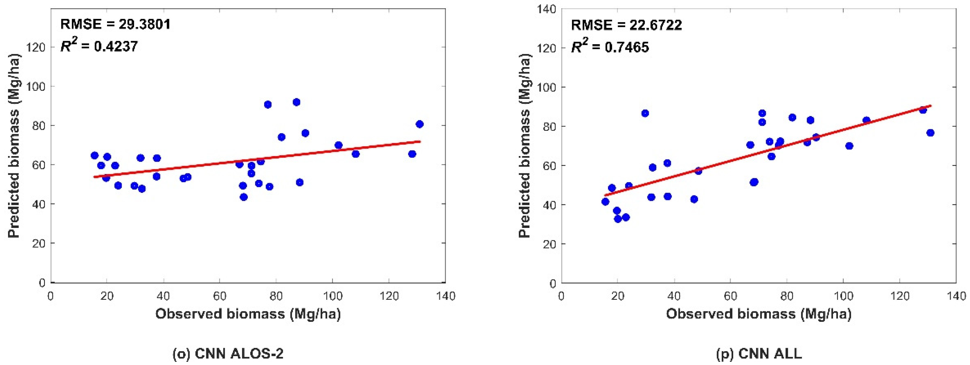
3.2.2. Machine-Learning Model

A total of 20% of the samples were randomly drawn to validate the accuracy of different machine-learning model. The data were divided into two parts for training and validation first, and the validation dataset was the same for each model. The results with optimal parameter were chosen for each model after repeating test. The scatter diagrams of different machine experiments are presented in Figure 5, showing the RMSE and R² values were performed based on Sentinel-2, Sentinel-1, ALOS-2, and the combination of all three sources. The result of a higher R² and a lower RMSE proves that the modeling effect was satisfactory. The combination of MSI and SAR showed a stronger ability of prediction accuracy than single sources.

Figure 5 shows the R² and RMSE values of the four models. In all four models, better performance was found with increasing data sources, followed by the performance using the Sentinel-2 data. This indicated that the vegetation index and biophysical predictors from Sentinel-2 were more helpful than those from other datasets. The SAR-derived predictors showed fewer effects than MSI predictors on the AGB predicted by the four models. In addition, compared to ALOS-2, Sentinel-1 performed slightly better. The L-band is known to be more sensitive than the C-band in AGB estimation. Nevertheless, we added SAR interference coherence to Sentinel-1 predicted variables, which increased the performance of the models with Sentinel-1 variables.

Regardless of whether the model was based on a single dataset or combined data, the CNN algorithm exhibited the highest prediction accuracy, while the MLR had the lowest (Figure 6). All nonparametric models were more accurate than parametric model represented by the linear regression model, indicating that the forest AGB and multisource remote-sensing parameters have a complicated nonlinear relationship. In the machine-learning models, the RF model performed better in prediction than that of the SVR model. The RF algorithm has a high tolerance to outliers and noise, and rarely exhibits the overfitting phenomenon; therefore, a high prediction accuracy could be achieved. Among the DL models, the Keras algorithm had better prediction results than machine-learning models for single SAR data source, while the accuracies of MSI and collaborative data were lower than that of machine-learning models. The accuracy improvement was more evident in the CNN model based on any data source.

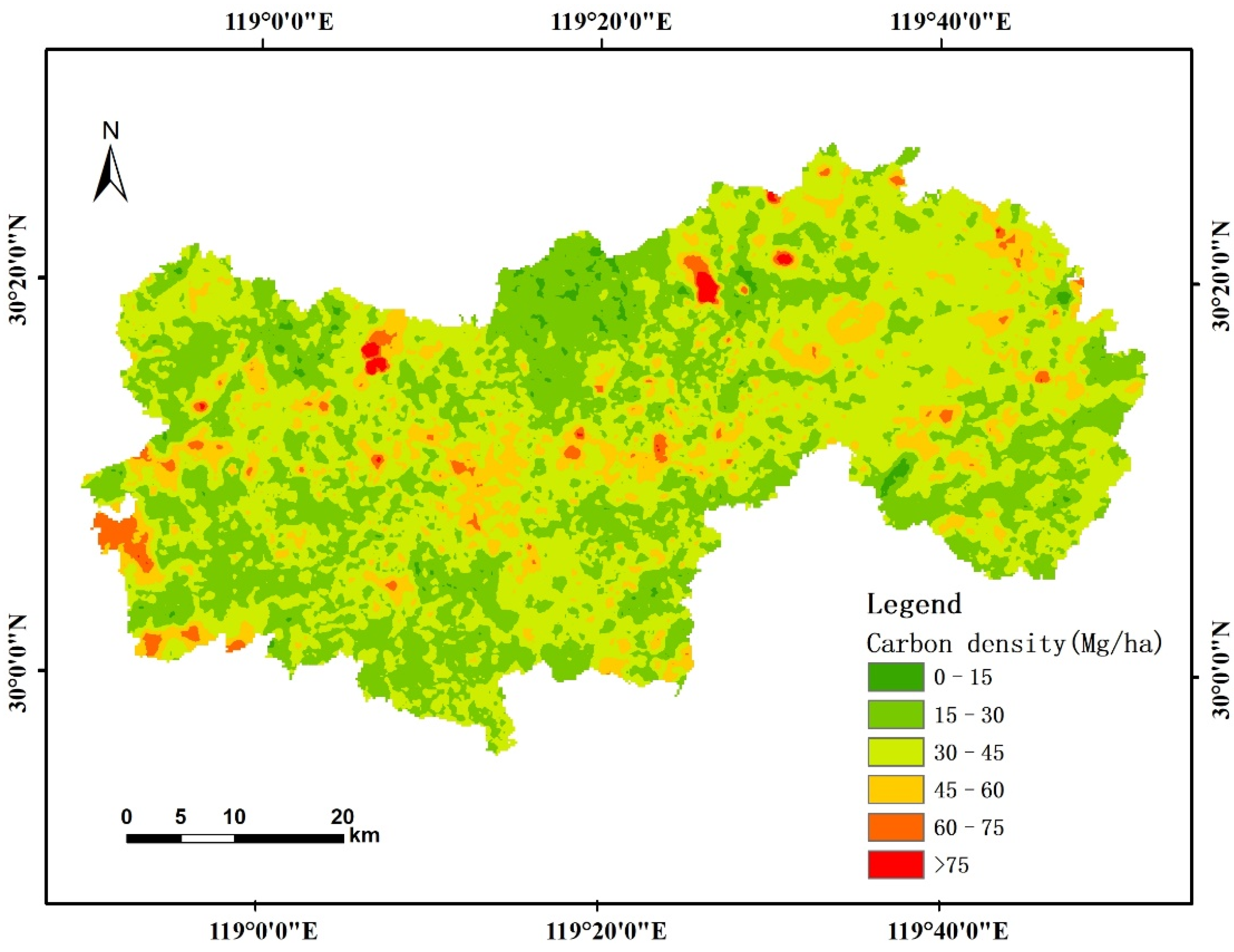
3.3. Mapping Spatial Distribution of Forest

The CNN estimation model exhibited the highest accuracy among the abovementioned methods. The regional forest AGB of the entire study area was obtained by applying the optimal model. Carbon density was calculated by the abovementioned method using forest AGB. Figure 5 shows a forest aboveground carbon-density map with spatial distribution patterns. As shown in Figure 7, the average carbon-density value was 32.10 Mg/ha, and most of that was concentrated at approximately 30–45 Mg/ha.

4. Discussion

4.1. Forest-Resource Inventory Data and Satellite Data

In this study, we propose different methods for modeling and mapping forest carbon density at a regional scale. As different environments and tree species exist in various areas, establishing a specific regional-scale model could provide more detailed and precise information, as well as improve the model estimation accuracy. The forest-resource inventory data contain information on various forest attributes, including not only DBH and tree height, which are the two most related variables to forest AGB [58], but also age, canopy density, soil type, altitude, and slope aspect, which are important in analyzing the influencing parameters of carbon spatial distribution.

In previous studies, forest AGB estimation using only optical data would reach saturation and limit the estimation results [59]. Combining optical and radar data can raise the upper limit and improve the estimation accuracy [22,60]. Optical data are effective for the classification of forest types and estimation of forest characteristic parameters, whereas radar data can penetrate the forest branches and leaves and predict the vertical structure of forests. To improve the accuracy of forest AGB estimation, radar data can be used as a supplement to optical data.

4.2. Variable Selection

Characteristic variables exhibiting a high correlation with AGB were chosen based on the physical significance of the attributes and correlation coefficients; the predictors with a weak correlation in the same category of redundancy parameters were eliminated. Optical remote sensing was found to have a stronger predictive ability than radar remote sensing in predicting AGB, and the characteristic variables showed a stronger correlation. This is primarily caused by the saturation of radar remote-sensing backscattering. This also indicated that the texture and interference information of radar data are more useful than backscattering information in predicting forest AGB, and that the texture feature can reduce the effect of spatial heterogeneity. The comparison of the Sentinel-1 and ALOS-2 data revealed that the L-band is more sensitive to forest AGB than the C-band, and it is more suitable for forest AGB prediction. This is consistent with the findings of previous studies [23,61], since longer wavelengths could penetrate the canopy, they can provide more information from the trunk and branches [62]. While interference coherence provides more vertical information about the forest. Moreover, HV polarization is more sensitive to forest AGB than HH, as cross-polarization is stronger than homo-polarization in vertical penetration.

In previous study, InSAR coherence is not commonly used as predictor variables for forest AGB estimation [62,63], but coherence can be used as good predictors. This is because the InSAR technique can obtain the interferometric phase and coherence coefficients that contain the information of the features, which improve the saturation point of biomass [64,65]. This study demonstrated the advantages of combining multiple sensor data sources for forest AGB prediction, and the limitations of using single remote-sensing predictors. The vegetation index of optical data, and the texture and coherence variables of radar data were the main variables of forest AGB estimation.

4.3. Model Comparison

This study proposed a DL model for estimating forest AGB and carbon storage. The nonlinear property of the DL model made it more accurate in estimating the forest AGB and performed better than the MLR model. The prediction of extreme forest AGB by the MLR model was unsatisfactory, which is consistent with the results of previous studies [66,67]. The RF algorithm is not subject to the problems of sample size, distribution, or optimal-model-parameter selection [34] and exhibited good performance in the estimation results. Compared with the RF and SVR models, the CNN model was more suitable for forest AGB estimation, while the estimation using Keras was less ideal, mainly because the experiment was performed using only 160 samples, which was a relatively small number of samples for achieving high prediction accuracy. The SVR model has more advantages in processing small sample sizes for prediction [68], whereas the RF model is not affected by sample size.

The DL model is widely known to be sensitive in the process of mesh design, parameter setting, and calculation. The algorithms can be difficult to handle, even though they have been applied for decades [69]. Therefore, the uncertainties in the chosen structures and input-window sizes were difficult to fully understand. In this study, we explored the uncertainty that existed mainly in neuron-number selection and parameter settings.

Certainly, there are some limitations in this paper. Environmental factors such as soil, climate, and hydrology have an impact on forest AGB estimation [67,70], which have not been considered in this paper, and this needs to be strengthened in future research. Future work can experiment and compare more deep-learning models in order to generate more complete and universal products for estimating forest AGB with multisource remote-sensing data. Finally, the results of the deep-learning models used to estimate AGB in this study suggest that further research is needed to better understand and apply deep learning in forest mapping.

5. Conclusions

Based on Sentinel-2 optical data, Sentinel-1 C-band SAR, and ALOS-2 L-band SAR, different algorithms, including MLR, SVR, RF, Keras, and CNN, were applied in this study to estimate the forest carbon density based on AGB and generate a map of carbon density. The performance of the results demonstrated that for the same predicted variables, the traditional MLR model could not accurately represent the nonlinear relationship between predictors and forest AGB, the accuracy of R² reached 0.3794 with three remote-sensing data, while the DL algorithm was found to be more efficient in carbon-density estimation with an R² of 0.7465. Thus, CNN can evidently be applied to carbon-density prediction and achieve ideal results if suitably adjusted. Consequently, some aspects of CNN should be further investigated in forest applications, and the development of DL may lead to a convenient and improved prediction.

References

1. Tang, H.; Hong, Q.; Xu, B. Landscape performance assessment of phase I of greenway around Qingshan Lake National Forest Park, Zhejiang Province. J. Zhejiang A&F Univ. 2020, 37, 1177–1185. [Google Scholar]
2. Chen, L.; Wang, Y.; Ren, C.; Zhang, B.; Wang, Z. Assessment of multi-wavelength SAR and multispectral instrument data for forest aboveground biomass mapping using random forest kriging. For. Ecol. Manag. 2019, 447, 12–25. [Google Scholar] [CrossRef]
3. Wu, M.; Dong, G.; Wang, Y.; Xiong, R.; Li, Y.; Cheng, W.; Fu, Z.; Fan, S. Estimation of forest aboveground carbon storage in Sichuan Miyaluo Nature Reserve based on remote sensing. Acta Ecol. Sin. 2020, 40, 621–628. [Google Scholar]
4. Liu, N.; Caldwell, P.V.; Dobbs, G.R.; Miniat, C.F.; Bolstad, P.V.; Nelson, S.A.C.; Sun, G. Forested lands dominate drinking water supply in the conterminous United States. Environ. Res. Lett. 2021, 16, 084008. [Google Scholar] [CrossRef]
5. Cheng, W.X.; Yang, C.J.; Zhou, W.C.; Liu, Y.C. Research summary of forest volume quantitative estimation based on remote sensing technology. J. Anhui Sci. 2009, 37, 7746–7750. [Google Scholar] [CrossRef]
6. Wang, X.; Shao, G.; Chen, H.; Lewis, B.J.; Qi, G.; Yu, D.; Zhou, L.; Dai, L. An Application of Remote Sensing Data in Mapping Landscape-Level Forest Biomass for Monitoring the Effectiveness of Forest Policies in Northeastern China. Environ. Manag. 2013, 52, 612–620. [Google Scholar] [CrossRef]
7. Mu, B.; Zhao, X.; Zhao, J.; Liu, N.; Si, L.; Wang, Q.; Sun, N.; Sun, M.; Guo, Y.; Zhao, S. Quantitatively Assessing the Impact of Driving Factors on Vegetation Cover Change in China’s 32 Major Cities. Remote Sens. 2022, 14, 839. [Google Scholar] [CrossRef]
8. Fu, Y. Aboveground biomass estimation and uncertainties assessing on regional scale with an improved model analysis method. Hubei For. Sci. Technol. 2018, 47, 1–4+38. [Google Scholar]
9. Liu, N.; Sun, P.; Caldwell, P.V.; Harper, R.; Liu, S.; Sun, G. Trade-off between watershed water yield and ecosystem productivity along elevation gradients on a complex terrain in southwestern China. J. Hydrol. 2020, 590, 125449. [Google Scholar] [CrossRef]
10. Bi, H.; Murphy, S.; Volkova, L.; Weston, C.; Fairman, T.; Li, Y.; Law, R.; Norris, J.; Lei, X.; Caccamo, G. Additive biomass equations based on complete weighing of sample trees for open eucalypt forest species in south-eastern Australia. For. Ecol. Manag. 2015, 349, 106–121. [Google Scholar] [CrossRef]
11. Vahtmae, E.; Kotta, J.; Lougas, L.; Kutser, T. Mapping spatial distribution, percent cover and biomass of benthic vegetation in optically complex coastal waters using hyperspectral CASI and multispectral Sentinel-2 sensors. Int. J. Appl. Earth Obs. Geoinf. 2021, 102, 102444. [Google Scholar] [CrossRef]
12. Pan, L.; Sun, Y.J.; Wang, Y.F. Estimation of aboveground biomass in a Chinese fir (Cunninghamia lanceolata) forest combining data of Sentinel-1 and Sentinel-2. J. Nanjing For. Univ. Nat. Sci. Ed. 2020, 44, 149–156. [Google Scholar]
13. Chrysafis, I.; Mallinis, G.; Tsakiri, M.; Patias, P. Evaluation of single-date and multi-seasonal spatial and spectral information of Sentinel-2 imagery to assess growing stock volume of a Mediterranean forest. Int. J. Appl. Earth Obs. Geoinf. 2019, 77, 1–14. [Google Scholar] [CrossRef]
14. Naidoo, L.; van Deventer, H.; Ramoelo, A.; Mathieu, R.; Nondlazi, B.; Gangat, R. Estimating above ground biomass as an indicator of carbon storage in vegetated wetlands of the grassland biome of South Africa. Int. J. Appl. Earth Obs. Geoinf. 2019, 78, 118–129. [Google Scholar] [CrossRef]
15. Jiang, M.; Ding, X.; Hanssen, R.F.; Malhotra, R.; Chang, L. Fast Statistically Homogeneous Pixel Selection for Covariance Matrix Estimation for Multitemporal InSAR. IEEE Trans. Geosci. Remote Sens. 2015, 53, 1213–1224. [Google Scholar] [CrossRef]
16. Jiang, M.; Guarnieri, A.M. Distributed Scatterer Interferometry With the Refinement of Spatiotemporal Coherence. Ieee Trans. Geosci. Remote Sens. 2020, 58, 3977–3987. [Google Scholar] [CrossRef]
17. Xiao, R.; Jiang, M.; Li, Z.; He, X. New insights into the 2020 Sardoba dam failure in Uzbekistan from Earth observation. Int. J. Appl. Earth Obs. Geoinf. 2022, 107, 102705. [Google Scholar] [CrossRef]
18. Tian, X.; Jiang, M.; Xiao, R.; Malhotra, R. Bias Removal for Goldstein Filtering Power Using a Second Kind Statistical Coherence Estimator. Remote Sens. 2018, 10, 1559. [Google Scholar] [CrossRef] [Green Version]
19. Dinh Ho Tong, M.; Thuy Le, T.; Rocca, F.; Tebaldini, S.; d’Alessandro, M.M.; Villard, L. Relating P-Band Synthetic Aperture Radar Tomography to Tropical Forest Biomass. IEEE Trans. Geosci. Remote Sens. 2014, 52, 967–979. [Google Scholar] [CrossRef]
20. Gholizadeh, A.; Misurec, J.; Kopackova, V.; Mielke, C.; Rogass, C. Assessment of Red-Edge Position Extraction Techniques: A Case Study for Norway Spruce Forests Using HyMap and Simulated Sentinel-2 Data. Forests 2016, 7, 226. [Google Scholar] [CrossRef] [Green Version]
21. Udali, A.; Lingua, E.; Persson, H.J. Assessing Forest Type and Tree Species Classification Using Sentinel-1 C-Band SAR Data in Southern Sweden. Remote Sens. 2021, 13, 3237. [Google Scholar] [CrossRef]
22. Vafaei, S.; Soosani, J.; Adeli, K.; Fadaei, H.; Naghavi, H.; Pham, T.D.; Bui, D.T. Improving Accuracy Estimation of Forest Aboveground Biomass Based on Incorporation of ALOS-2 PALSAR-2 and Sentinel-2A Imagery and Machine Learning: A Case Study of the Hyrcanian Forest Area (Iran). Remote Sens. 2018, 10, 172. [Google Scholar] [CrossRef] [Green Version]
23. Stelmaszczuk-Gorska, M.A.; Urbazaev, M.; Schmullius, C.; Thiel, C. Estimation of Above-Ground Biomass over Boreal Forests in Siberia Using Updated In Situ, ALOS-2 PALSAR-2, and RADARSAT-2 Data. Remote Sens. 2018, 10, 1550. [Google Scholar] [CrossRef] [Green Version]
24. Laurin, G.V.; Pirotti, F.; Callegari, M.; Chen, Q.; Cuozzo, G.; Lingua, E.; Notarnicola, C.; Papale, D. Potential of ALOS2 and NDVI to Estimate Forest Above-Ground Biomass, and Comparison with Lidar-Derived Estimates. Remote Sens. 2017, 9, 18. [Google Scholar] [CrossRef] [Green Version]
25. Santoro, M.; Cartus, O. Research Pathways of Forest Above-Ground Biomass Estimation Based on SAR Backscatter and Interferometric SAR Observations. Remote Sens. 2018, 10, 608. [Google Scholar] [CrossRef] [Green Version]
26. Wu, C.; Tao, H.; Zhai, M.; Lin, Y.; Wang, K.; Deng, J.; Shen, A.; Gan, M.; Li, J.; Yang, H. Using nonparametric modeling approaches and remote sensing imagery to estimate ecological welfare forest biomass. J. For. Res. 2018, 29, 151–161. [Google Scholar] [CrossRef]
27. Ndikumana, E.; Dinh Ho Tong, M.; Hai Thu Dang, N.; Baghdadi, N.; Courault, D.; Hossard, L.; El Moussawi, I. Estimation of Rice Height and Biomass Using Multitemporal SAR Sentinel-1 for Camargue, Southern France. Remote Sens. 2018, 10, 1394. [Google Scholar] [CrossRef] [Green Version]
28. Vamosi, S.; Reutterer, T.; Platzer, M. A deep recurrent neural network approach to learn sequence similarities for user-identification. Decis. Support Syst. 2022, 155, 113718. [Google Scholar] [CrossRef]
29. Castro, W.; Marcato, J., Jr.; Polidoro, C.; Osco, L.P.; Goncalves, W.; Rodrigues, L.; Santos, M.; Jank, L.; Barrios, S.; Valle, C.; et al. Deep Learning Applied to Phenotyping of Biomass in Forages with UAV-Based RGB Imagery. Sensors 2020, 20, 4802. [Google Scholar] [CrossRef]
30. Ghosh, S.M.; Behera, M.D. Aboveground biomass estimates of tropical mangrove forest using Sentinel-1 SAR coherence data-The superiority of deep learning over a semi-empirical model. Comput. Geosci. 2021, 150, 104737. [Google Scholar] [CrossRef]
31. Xing, W.; Qian, Y.; Guan, X.; Yang, T.; Wu, H. A novel cellular automata model integrated with deep learning for dynamic spatio-temporal land use change simulation. Comput. Geosci. 2020, 137, 104430. [Google Scholar] [CrossRef]
32. Kim, J.; Kim, H.; Jeon, H.; Jeong, S.H.; Song, J.Y.; Vadivel, S.K.P.; Kim, D.J. Synergistic Use of Geospatial Data for Water Body Extraction from Sentinel-1 Images for Operational Flood Monitoring across Southeast Asia Using Deep Neural Networks. Remote Sens. 2021, 13, 4759. [Google Scholar] [CrossRef]
33. Li, X.H. Using “random forest” for classification and regression. Chin. J. Appl. Entomol. 2013, 50, 1190–1197. [Google Scholar]
34. Huang, X.; Wang, Z.; Xu, X. Comparison of fitting approaches with biomass expansion factor equations. J. Zhejiang A&F Univ. 2017, 34, 775–781. [Google Scholar]
35. Li, S.-M.; Yang, C.-Q.; Wang, H.-N.; Ge, L.-Q. Carbon storage of forest stands in Shandong Province estimated by forestry inventory data. Ying Yong Sheng Tai Xue Bao J. Appl. Ecol. 2014, 25, 2215–2220. [Google Scholar]
36. Saatchi, S.S.; Harris, N.L.; Brown, S.; Lefsky, M.; Mitchard, E.T.A.; Salas, W.; Zutta, B.R.; Buermann, W.; Lewis, S.L.; Hagen, S.; et al. Benchmark map of forest carbon stocks in tropical regions across three continents. Proc. Natl. Acad. Sci. USA 2011, 108, 9899–9904. [Google Scholar] [CrossRef] [Green Version]
37. Liu, H.; Lei, R. Research Methods and Advances of Carbon Storage and Balance in Forest Ecosystems of China. Acta Bot. Boreali-Occident. Sin. 2005, 25, 835–843. [Google Scholar]
38. Liu, Y.; Zhang, Y.; Liu, S. Aboveground carbon stock evaluation with different restoration approaches using tree ring chronosequences in Southwest China. For. Ecol. Manag. 2012, 263, 39–46. [Google Scholar] [CrossRef]
39. Dixon, R.K. Carbon Pools and Flux of Global Forest Ecosystems. Science 1994, 265, 171. [Google Scholar] [CrossRef]
40. Tien Dat, P.; Yokoya, N.; Xia, J.; Nam Thang, H.; Nga Nhu, L.; Thi Thu Trang, N.; Thi Huong, D.; Thuy Thi Phuong, V.; Tien Duc, P.; Takeuchi, W. Comparison of Machine Learning Methods for Estimating Mangrove Above-Ground Biomass Using Multiple Source Remote Sensing Data in the Red River Delta Biosphere Reserve, Vietnam. Remote Sens. 2020, 12, 1334. [Google Scholar] [CrossRef] [Green Version]
41. Tian, X.; Malhotra, R.; Xu, B.; Qi, H.; Ma, Y. Modeling Orbital Error in InSAR Interferogram Using Frequency and Spatial Domain Based Methods. Remote Sens. 2018, 10, 508. [Google Scholar] [CrossRef] [Green Version]
42. Vieilledent, G.; Vaudry, R.; Andriamanohisoa, S.; Rakotonarivo, O.S.; Randrianasolo, H.Z.; Razafindrabe, H.N.; Rakotoarivony, C.B.; Rasamoelina, J.E. A universal approach to estimate biomass and carbon stock in tropical forests using generic allometric models. Ecol. Appl. 2012, 22, 572–583. [Google Scholar] [CrossRef] [PubMed]
43. Xu, Z.Y. Forest biomass retrieval based on Sentinel-1A and Landsat 8 image. J. Cent. South Univ. For. Technol. 2020, 40, 147–155. [Google Scholar] [CrossRef]
44. Godinho Cassol, H.L.; de Brito Carreiras, J.M.; Moraes, E.C.; Oliveira e Cruz de Aragao, L.E.; de Jesus Silva, C.V.; Quegan, S.; Shimabukuro, Y.E. Retrieving Secondary Forest Aboveground Biomass from Polarimetric ALOS-2 PALSAR-2 Data in the Brazilian Amazon. Remote Sens. 2019, 11, 59. [Google Scholar] [CrossRef] [Green Version]
45. Camps-Valls, G.; Gomez-Chova, L.; Munoz-Mari, J.; Vila-Frances, J.; Amoros-Lopez, J.; Calpe-Maravilla, J. Retrieval of oceanic chlorophyll concentration with relevance vector machines. Remote Sens. Environ. 2006, 105, 23–33. [Google Scholar] [CrossRef]
46. Du, H.; Mao, F.; Zhou, G.; Li, X.; Xu, X.; Ge, H.; Cui, L.; Liu, Y.; Zhu, D.e.; Li, Y. Estimating and Analyzing the Spatiotemporal Pattern of Aboveground Carbon in Bamboo Forest by Combining Remote Sensing Data and Improved BIOME-BGC Model. IEEE J. Sel. Top. Appl. Earth Obs. Remote Sens. 2018, 11, 2282–2295. [Google Scholar] [CrossRef]
47. Axelsson, C.; Skidmore, A.K.; Schlerf, M.; Fauzi, A.; Verhoef, W. Hyperspectral analysis of mangrove foliar chemistry using PLSR and support vector regression. Int. J. Remote Sens. 2013, 34, 1724–1743. [Google Scholar] [CrossRef]
48. Breiman, L. Random forests. Mach. Learn. 2001, 45, 5–32. [Google Scholar] [CrossRef] [Green Version]
49. Lausch, A.; Erasmi, S.; King, D.J.; Magdon, P.; Heurich, M. Understanding Forest Health with Remote Sensing-Part II—A Review of Approaches and Data Models. Remote Sens. 2017, 9, 129. [Google Scholar] [CrossRef] [Green Version]
50. Osah, S.; Acheampong, A.A.; Fosu, C.; Dadzie, I. Deep learning model for predicting daily IGS zenith tropospheric delays in West Africa using TensorFlow and Keras. Adv. Space Res. 2021, 68, 1243–1262. [Google Scholar] [CrossRef]
51. Moolayil, J. Learn Keras for Deep Neural Networks: A Fast-Track Approach to Modern Deep Learning with Python; Apress: New York, NY, USA, 2019. [Google Scholar]
52. Li, Y.; Zhang, H.; Xue, X.; Jiang, Y.; Shen, Q. Deep learning for remote sensing image classification: A survey. Wiley Interdiscip. Rev. Data Min. Knowl. Discov. 2018, 8, e1264. [Google Scholar] [CrossRef] [Green Version]
53. Dong, L.; Du, H.; Han, N.; Li, X.; Zhu, D.e.; Mao, F.; Zhang, M.; Zheng, J.; Liu, H.; Huang, Z.; et al. Application of Convolutional Neural Network on Lei Bamboo Above-Ground-Biomass (AGB) Estimation Using Worldview-2. Remote Sens. 2020, 12, 958. [Google Scholar] [CrossRef] [Green Version]
54. Fu, G.; Liu, C.; Zhou, R.; Sun, T.; Zhang, Q. Classification for High Resolution Remote Sensing Imagery Using a Fully Convolutional Network. Remote Sens. 2017, 9, 498. [Google Scholar] [CrossRef] [Green Version]
55. Saud, P.; Lynch, T.B.; Anup, K.C.; Guldin, J.M. Using quadratic mean diameter and relative spacing index to enhance height-diameter and crown ratio models fitted to longitudinal data. Forestry 2016, 89, 215–229. [Google Scholar] [CrossRef] [Green Version]
56. Sarker, L.R.; Nichol, J.E. Improved forest biomass estimates using ALOS AVNIR-2 texture indices. Remote Sens. Environ. 2011, 115, 968–977. [Google Scholar] [CrossRef]
57. Ma, J.; Xiao, X.; Qin, Y.; Chen, B.; Hu, Y.; Li, X.; Zhao, B. Estimating aboveground biomass of broadleaf, needleleaf, and mixed forests in Northeastern China through analysis of 25-m ALOS/PALSAR mosaic data. For. Ecol. Manag. 2017, 389, 199–210. [Google Scholar] [CrossRef]
58. Rutishauser, E.; Noor’an, F.; Laumonier, Y.; Halperin, J.; Rufi’ie; Hergoualc’h, K.; Verchot, L. Generic allometric models including height best estimate forest biomass and carbon stocks in Indonesia. For. Ecol. Manag. 2013, 307, 219–225. [Google Scholar] [CrossRef]
59. Gao, Y.; Lu, D.; Li, G.; Wang, G.; Chen, Q.; Liu, L.; Li, D. Comparative Analysis of Modeling Algorithms for Forest Aboveground Biomass Estimation in a Subtropical Region. Remote Sens. 2018, 10, 627. [Google Scholar] [CrossRef] [Green Version]
60. Laurin, G.V.; Balling, J.; Corona, P.; Mattioli, W.; Papale, D.; Puletti, N.; Rizzo, M.; Truckenbrodt, J.; Urban, M. Above-ground biomass prediction by Sentinel-1 multitemporal data in central Italy with integration of ALOS2 and Sentinel-2 data. J. Appl. Remote Sens. 2018, 12, 016008. [Google Scholar] [CrossRef]
61. Balzter, H.; Baker, J.R.; Hallikainen, M.; Tomppo, E. Retrieval of timber volume and snow water equivalent over a Finnish boreal forest from airborne polarimetric Synthetic Aperture Radar. Int. J. Remote Sens. 2002, 23, 3185–3208. [Google Scholar] [CrossRef] [Green Version]
62. Sadeghi, Y.; St-Onge, B.; Leblon, B.; Prieur, J.-F.; Simard, M. Mapping boreal forest biomass from a SRTM and TanDEM-X based on canopy height model and Landsat spectral indices. Int. J. Appl. Earth Obs. Geoinf. 2018, 68, 202–213. [Google Scholar] [CrossRef]
63. Hunter, M.O.; Keller, M.; Victoria, D.; Morton, D.C. Tree height and tropical forest biomass estimation. Biogeosciences 2013, 10, 8385–8399. [Google Scholar] [CrossRef] [Green Version]
64. Shi, J.; Du, Y.; Du, J.; Jiang, L.; Chai, L.; Mao, K.; Xu, P.; Ni, W.; Xiong, C.; Liu, Q.; et al. Progresses on microwave remote sensing of land surface parameters. Sci. China-Earth Sci. 2012, 55, 1052–1078. [Google Scholar] [CrossRef]
65. Santoro, M.; Shvidenko, A.; McCallum, I.; Askne, J.; Schmullius, C. Properties of ERS-1/2 coherence in the Siberian boreal forest and implications for stem volume retrieval. Remote Sens. Environ. 2007, 106, 154–172. [Google Scholar] [CrossRef]
66. Fuchs, H.; Magdon, P.; Kleinn, C.; Flessa, H. Estimating aboveground carbon in a catchment of the Siberian forest tundra: Combining satellite imagery and field inventory. Remote Sens. Environ. 2009, 113, 518–531. [Google Scholar] [CrossRef]
67. Zhu, Y.; Feng, Z.; Lu, J.; Liu, J. Estimation of Forest Biomass in Beijing (China) Using Multisource Remote Sensing and Forest Inventory Data. Forests 2020, 11, 163. [Google Scholar] [CrossRef] [Green Version]
68. Souza, G.S.A.d.; Soares, V.P.; Leite, H.G.; Gleriani, J.M.; do Amaral, C.H.; Ferraz, A.S.; Silveira, M.V.d.F.; Santos, F.C.d.; Velloso, S.G.S.; Domingues, G.F.; et al. Multi-sensor prediction of Eucalyptus stand volume: A support vector approach. ISPRS J. Photogramm. Remote Sens. 2019, 156, 135–146. [Google Scholar] [CrossRef]
69. Jia, M.; Tong, L.; Chen, Y.; Wang, Y.; Zhang, Y. Rice biomass retrieval from multitemporal ground-based scatterometer data and RADARSAT-2 images using neural networks. J. Appl. Remote Sens. 2013, 7, 073509. [Google Scholar] [CrossRef]
70. Narine, L.L.; Popescu, S.C.; Malambo, L. Synergy of ICESat-2 and Landsat for Mapping Forest Aboveground Biomass with Deep Learning. Remote Sens. 2019, 11, 1503. [Google Scholar] [CrossRef]
Figure 1. Spatial distribution of field sampling sites and location of study area in Zhejiang.
Remotesensing 14 03022 g001
Figure 2. Graphs depicting the carbon-density range and frequency of plots in the study area.
Remotesensing 14 03022 g002
Figure 3. The importance of predictor variables, 20 variables with a high Pearson correlation coefficient were selected to observe the correlation among variables.
Remotesensing 14 03022 g003
Figure 4. Scatter plots showing the accuracies of the MLR models obtained using the following remote-sensing data: (a) Sentinel-2, (b) Sentinel-1, (c) ALOS-2, and (d) all three data sources. The blue dots indicate a pair of corresponding predicted and observed values. The red line indicates the trend line.
Remotesensing 14 03022 g004
Figure 5. Scatter plots showing the predicted and observed AGB obtained from data validation using the four models. The figures depict the different predictors, including (a,e,i,m) Sentinel-2 data; (b,f,j,n) Sentinel-1 data; (c,g,k,o) ALOS-2 data; and (d,h,l,p) combination of all three datasets. The blue dots indicate a pair of corresponding predicted and observed values. The red line indicates the trend line.
Remotesensing 14 03022 g005aRemotesensing 14 03022 g005bRemotesensing 14 03022 g005c
Figure 6. The RMSE comparison of five different algorithms by validation data.
Remotesensing 14 03022 g006
Figure 7. Map showing the carbon-density distribution in the study area determined using CNN algorithms.
Remotesensing 14 03022 g007