Genus-Level Mapping of Invasive Floating Aquatic Vegetation Using Sentinel-2 Satellite Remote Sensing

Abstract

Invasive floating aquatic vegetation negatively impacts wetland ecosystems and mapping this vegetation through space and time can aid in designing and assessing effective control strategies. Current remote sensing methods for mapping floating aquatic vegetation at the genus level relies on airborne imaging spectroscopy, resulting in temporal gaps because routine hyperspectral satellite coverage is not yet available. Here we achieved genus level and species level discrimination between two invasive aquatic vegetation species using Sentinel 2 multispectral satellite data and machine-learning classifiers in summer and fall. The species of concern were water hyacinth (Eichornia crassipes) and water primrose (Ludwigia spp.). Our classifiers also identified submerged and emergent aquatic vegetation at the community level. Random forest models using Sentinel-2 data achieved an average overall accuracy of 90%, and class accuracies of 79–91% and 85–95% for water hyacinth and water primrose, respectively. To our knowledge, this is the first study that has mapped water primrose to the genus level using satellite remote sensing. Sentinel-2 derived maps compared well to those derived from airborne imaging spectroscopy and we also identified misclassifications that can be attributed to the coarser Sentinel-2 spectral and spatial resolutions. Our results demonstrate that the intra-annual temporal gaps between airborne imaging spectroscopy observations can be supplemented with Sentinel-2 satellite data and thus, rapidly growing/expanding vegetation can be tracked in real time. Such improvements have potential management benefits by improving the understanding of the phenology, spread, competitive advantages, and vulnerabilities of these aquatic plants.

1. Introduction

Invasive floating aquatic vegetation (FAV) species are a global concern due to their negative impacts on fragile wetland ecosystem processes such as nutrient cycling, hydrology, and energy budgets [1,2,3,4]. Their introduction threatens ecosystem biodiversity and function, and often results in economic impact on fisheries, hydropower generation, and transportation services [5,6,7]. Understanding invasion pathways, processes, impacts, and triggers of change is an essential step in effective wetland management and is dependent on accurate mapping of vegetation and species prevalence through time [8].

Satellite remote sensing is a favored tool for monitoring invasive vegetation due to its synoptic views and repeat coverage; however, discrimination of multiple aquatic species in areas of high spatio-temporal complexity is often difficult due to spectral similarity between species and high spectral variation within a class [9,10,11]. Imaging spectroscopy has historically been the favored tool for mapping vegetation at the species or genus level because it offers high spectral resolution capable of discriminating between multiple aquatic species within the same functional type [12,13,14,15,16]. Airborne imaging spectroscopy (AIS) commonly has a high spatial resolution, which is important for mapping multiple FAV species that often co-occur within the same patch [13,17,18]. However, spaceborne imaging spectrometers with systematic, repeat sampling capabilities are currently rare and commercial AIS campaigns to collect such data are expensive—often resulting in annual and intra-annual data gaps. Such gaps hinder the ability to relate invasive species distribution to environmental and anthropogenic drivers of change during the growing season [19]. Newer multispectral satellites such as Sentinel-2A and B (S2) have a repeat period of 5 days at improved spectral and spatial resolutions compared to older multispectral satellites often used in wetland studies, such as Landsat or MODIS. This makes Sentinel-2 an attractive contender for mapping FAV species that are mobile and rapidly expand throughout the growing season.

The Sentinel-2 sensors provide the opportunity to discriminate between multiple FAV at the species and genus level throughout the growing season because of their high revisit frequency and high spatial resolution along with additional bands (relative to Landsat) that are intrinsically linked to vegetation traits [20]. Sentinel-2 has been used to distinguish between multiple emergent aquatic vegetation species (e.g., Spartina alterniflora, Phragmites australis) but the potential to spectrally discriminate between different types of FAV has yet to be determined [21,22]. Although Sentinel-2 has previously been used to map invasive FAV, such as water hyacinth, most study sites in the literature focus on relatively homogenous environments and community types, or target only one invasive species [23,24,25]. These prior studies also do not demonstrate the extent of Sentinel-2′s utility across a range of environments, nor do they differentiate floating vegetation at the genus or species-level.

The Sacramento-San Joaquin Delta (henceforth the Delta) is an extensively modified wetland system comprising multiple tidally influenced habitat types, including open lake-like and channelized riverine environments. The spatial heterogeneity and range of wetland environments in the Delta make it a unique setting for testing the potential of Sentinel-2 to distinguish FAV at the species or genus level, while simultaneously mapping submerged and emergent aquatic vegetation at the community level to provide holistic wetland maps that can inform and assess management actions. Currently, aquatic vegetation in the Delta is mapped to the species, genus, and community level using annual AIS acquisitions [14,26]. However, the imagery is costly and thus only consists of one annual snapshot per year, which does not allow for intra-annual tracking of aquatic vegetation composition and coverage. At times, lack of funding has resulted in annual data gaps as well, further increasing the temporal gaps.

Here, we demonstrate for the first time that separation between invasive FAV at the genus and species level is possible using Sentinel-2. We compared our Sentinel-2 maps to those derived from AIS; the current near-operational method employed for aquatic mapping in the Delta. Our classifiers distinguish between invasive FAV water hyacinth (Pontederia crassipes; formerly Eichornia crassipes) and water primrose (Ludwigia spp.) and identify submerged and emergent aquatic vegetation at the community level for both summer and fall imagery, demonstrating that the intra-annual temporal gap can be closed, and rapidly expanding vegetation can be tracked throughout the growing season. Such improvements have multiple possible management benefits. For example, the State of California spends millions of dollars each year to control IAV in the Delta and costs are likely to continue to rise [27]. Gaining a better understanding of invasive FAV distribution and spread within the year can lead to more informed and effective control strategies.

2. Materials and Methods

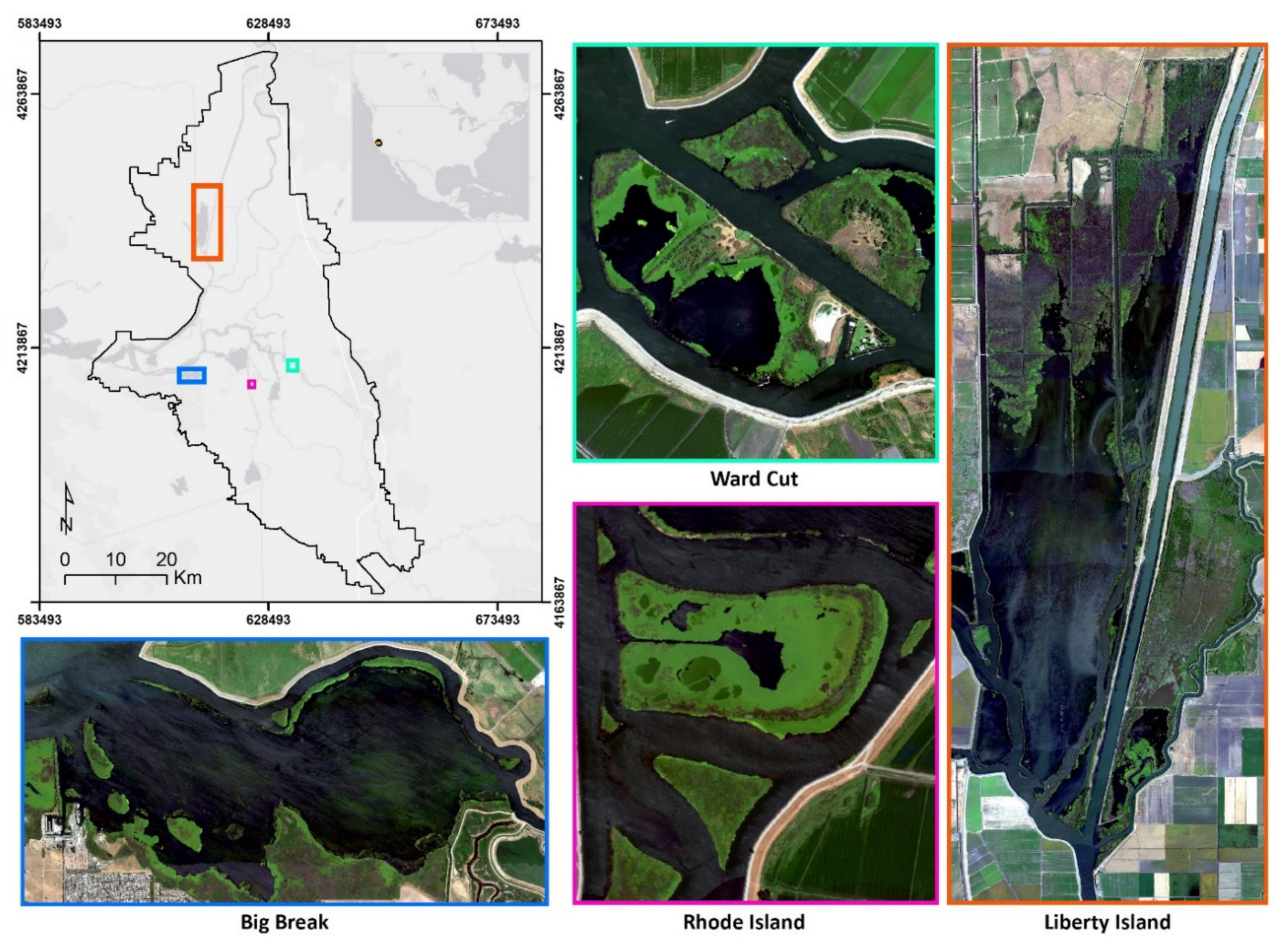
2.1. Experimental Design

Two floating aquatic macrophytes, water hyacinth (Pontederia crassipes) and water primrose (Ludwigia spp.), were targeted in this study. Water primrose, although nominally rooted, develops adventitious roots that can draw nutrients directly from the water. This allows water primrose to form floating canopies that extend several meters into the channel from the shore [28]. In contrast, water hyacinth is truly free-floating aquatic macrophyte—often anchoring itself to nearby emergent vegetation [29]. Both are among some of the most invasive aquatic macrophytes globally and are frequently referred to as ‘ecosystem engineers’ because of their ability to alter physical, biological, and chemical processes to their benefit [7,30,31]. For these reasons, we focused our extension of mapping capabilities on these two FAV aquatic macrophytes. Overall, our classification scheme comprises 8 classes—water hyacinth, water primrose, emergent aquatic vegetation (EAV), submerged aquatic vegetation (SAV), riparian vegetation, open water, non-photosynthetic vegetation (NPV), and soil (Figure 1 and

Table 1. Target classes and their descriptions.

Map Class	Description
Water Hyacinth	Pontederia crassipes
Water Primrose	Ludwigia spp.
Emergent Vegetation (EAV)	Cattail (Typha spp.) Common reed (Phragmites australis) Tule (Schoenoplectus spp.)
Riparian	For example: Willow species (Salix spp.), Oak species (Quercus spp.), and Cottonwood (Populus spp.)
Submerged Aquatic Vegetation (SAV)	Algae mats Brazilian waterweed (Egeria densa) Coontail (Ceratophyllum demersum) Curly leaf pondweed (Pomatogedon crispus) Fanwort (Cabomba caroliniana) Sago pondweed (Stuckenia pectinata) Watermilfoil (Myriophyllum spicatum) Waterweed (Elodea canadensis)
Non-Photosynthetic Vegetation (NPV)	Senescent or dead vegetation
Soil	Soil
Water	Water

). Figure 1 depicts the difference in spectral response between Sentinel-2 and AIS datasets for the target vegetation classes, further descriptions of the AIS instruments used here are in Section 2.3.

This study was conducted for the Delta, which is the hub of California’s water system spanning approximately 2220 km² in Northern and Central California. It is a heavily engineered system comprising a diverse network of channels and freshwater tidal marshes at the confluence of the Sacramento and the San Joaquin rivers (Figure 2) The Delta is also recognized as one of the most invaded estuaries in the world [33]. In the past few decades, water primrose and water hyacinth have negatively impacted water quality, water pumping, and native species, and there are ongoing efforts to control persistence and spread [27,34,35].

As part of the control and monitoring programs, AIS efforts to map these invasive floating species have been led by the Center of Spatial Technologies and Remote Sensing (CSTARS) at UC Davis from 2004–2008 and 2014–2021 [13,14,26,36,37]. An imaging spectrometer is flown on a low-altitude aircraft collecting high spatial resolution (~1.7–3 m pixels) and high spectral quality data. These data are used to prepare maps for California State Agencies and for assessing annual invasive species spread and community dynamics.

To evaluate the potential of Sentinel-2 for filling intra-annual data gaps, we compared the performance of a machine learning classifier using Sentinel-2 data to the current state-of-the-art approach for FAV mapping in the Delta derived from AIS [37]. To compare the two products, we identified the closest Sentinel-2 overpass to AIS acquisition with low cloud cover, we refer to these date pairs as “match up dates” that included fall 2018, fall 2019, and summer 2020 (

Table 2. Match-up dates and tidal ranges ¹ for corresponding imaging spectrometer acquisitions and Sentinel-2 over passes.

Match up Date	Imaging Spectrometer Acquisition Date	Closest Sentinel-2 Image Date	Imaging Spectrometer	Sentinel-2 Sensor	Tidal Range AIS 1 (m)	Tidal Range S2 (m)
Fall 2018	6–9 October 2018	7 October 2018	HyMap	S2B	0.01–0.25	0.49–0.64
Fall 2019	23–27 September 2019	2 October 2019	HyMap	S2B	0.01–1.02	0.28–0.39
Summer 2020	15–18 July 2020	18 July 2020	Fenix 1K	S2B	0.01–0.37	0.17–0.30

¹ Tidal ranges were downloaded from NOAA for the sensors at Antioch and Rio Vista (Station ID: 9415064 and 9415316, respectively). The ranges include measurements from stations.

). We labeled our mapping efforts FAV genus-level because multiple Ludwigia species are present in the Delta, but the exact number is unknown; they are difficult to visually distinguish in the field let alone from space.

While we mapped the entire Delta and made Delta-wide comparisons, for visualization and demonstration, map results are presented for four smaller sub-regions representative of the range of different habitat types in the Delta (Figure 2). Big Break is a brackish, shallow flooded island located downstream of the confluence of the Sacramento and San Joaquin Rivers. Liberty Island, an abandoned, flooded island, is a freshwater site influenced by the Sacramento River. Rhode Island and Ward Cut are islands along the San Joaquin River, that include a diverse mix of upland riparian and freshwater marsh habitats with large areas of deep open water bound by levees.

2.2. Acquisition and Pre-Processing of Sentinel-2 Imagery

Level-1C (L1C) top of atmosphere (TOA) reflectance products for Sentinel-2 tiles capturing the legal Delta boundary (10SFH, 10SFG and 10SEH) were downloaded from the Copernicus Open Access Hub for each of the three match-up dates listed in Table 2. Products were atmospherically corrected to Level-2A (L2A) bottom of atmosphere reflectance (BOA) using Sen2Cor version 2A and 2B to collect information in 13 spectral bands at 10, 20, and 60 m resolutions (

Table 3. Sentinel-2 band characteristics. Asterix indicates band was not used during classification.

Sentinel-2 Bands	Wavelengths (μm)	Spatial Resolution (m)
Band 1—Coastal Aerosol	0.430–0.457	60
Band 2—Blue	0.440–0.538	10
Band 3—Green	0.537–0.582	10
Band 4—Red	0.646–0.684	10
Band 5—Vegetation Red Edge 1	0.694–0.713	20
Band 6—Vegetation Red Edge 2	0.731–0.749	20
Band 7—Vegetation Red Edge 3	0.769–0.797	20
Band 8—NIR	0.785–0.900	10
Band 8A—Narrow NIR *	0.849–0.881	20
Band 9—Water Vapor *	0.932–0.958	60
Band 10—Cirrus *	1.337–1.412	60
Band 11—SWIR 1	1.539–1.682	20
Band 12—SWIR 2	2.078–2.320	20

). The Sen2r 1.4.0 R package was used to resample 20–60 m bands to a 10 m spatial resolution, mosaic tiles, and convert products from their native SAFE file format to ENVI files [38].

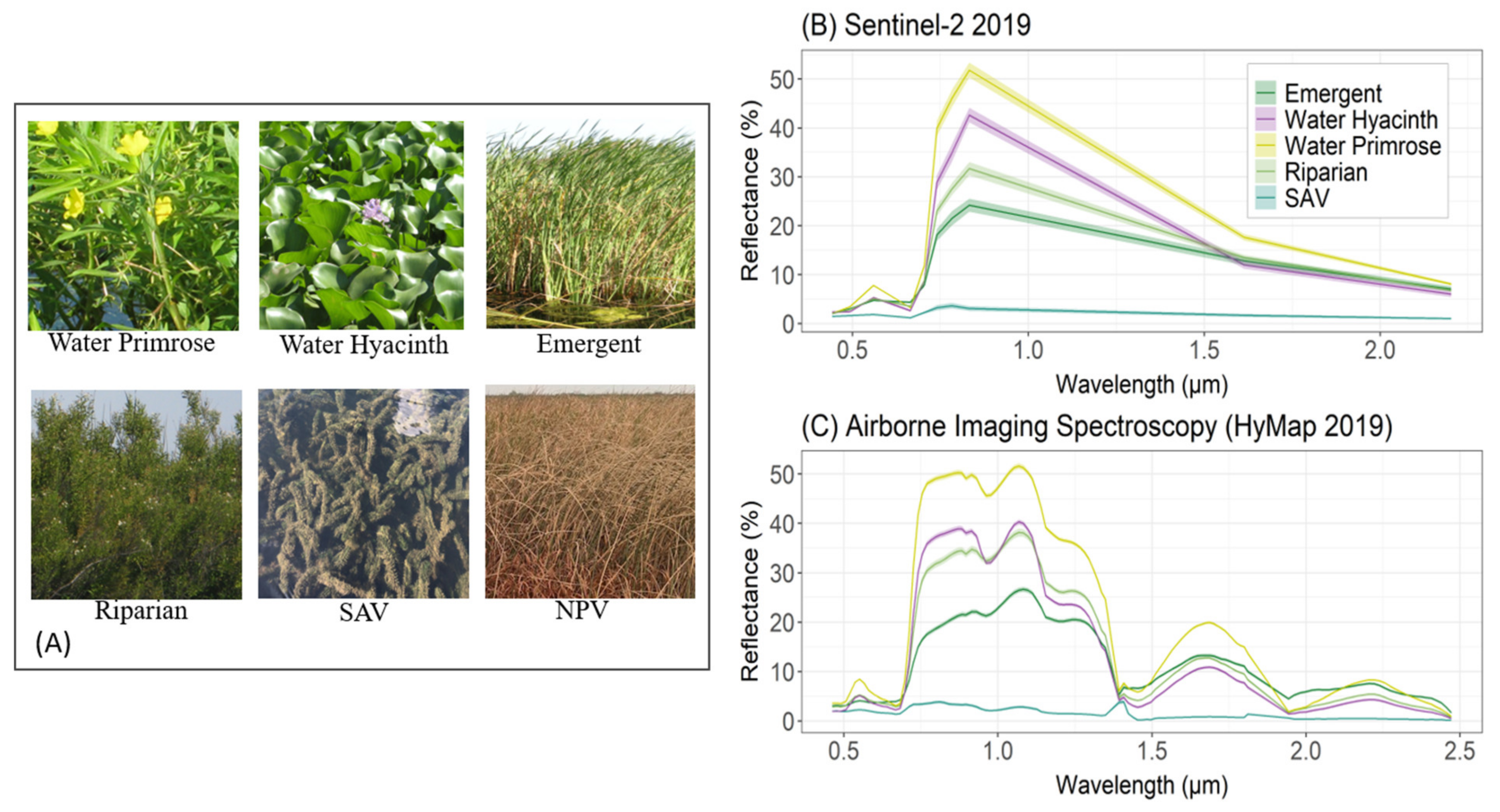
2.3. Imaging Spectroscopy Acquisitions and Classification Process

In fall 2018 and 2019, HyMap imaging spectroscopy data were collected over the Delta at a 1.7 × 1.7 m ground resolution in 126 bands (400–2500 nm, bandwidth ~15 nm) with a 20% overlap in flightlines by HyVista Corporation (Sydney, Australia). HyVista performed atmospheric calibration and delivered the data to CSTARS at UC Davis with geo-location files (GLT) for further processing. In July of 2020, SpecTIR LLC (Reno, NV, USA), flew their Fenix 1K hyperspectral imager over the Delta. The Fenix sensor measures 323 spectral bands across the visible to shortwave infrared spectrum (397–2450 nm) at a nominal spatial resolution of 2 × 2 m. SpecTIR also provided data to CSTARS after atmospheric calibration and included geographic lookup table files to associate each pixel with a geographic location. All airborne spectroscopy campaigns were conducted during low tide and flown to minimize sun glint.

Locations of aquatic vegetation species, riparian vegetation, and water were collected within a two-week window of image acquisition (~800–2000 points per campaign) using handheld high precision (sub-meter accuracy) GeoXT and GeoXH Trimble DGPS units (Trimble Navigation Limited, Sunnyvale, CA, USA) with Wide Area Augmentation System (WAAS) differential correction. Each location marks a dominant species, along with information on patch size, percent cover of each species present, and vegetation condition. Patch width and length are labeled as small (3–5 m), medium (5–10 m), large (10–15 m), and extra-large (>15 m). Classification training and validation polygons are then created through photointerpretation using field collected points and ground reference photos as a reference, in ArcMap (ArcGIS 10, Redlands, CA, USA) [37].

CSTARS classifies the spectroscopy data using a random forest algorithm trained and validated with the field collected reference data. A separate random forest model is developed for each campaign. Input data include a suite of spectral indexes, spectral angle mapper rule images, linear spectral unmixing fractional cover, and continuum removal of absorption features [39]. The polygons are randomly split into 50/50 training and validation data. Class accuracies were evaluated using confusion matrices which report an overall accuracy, user’s and producer’s accuracies, and the Kappa statistic [40,41]. The overall accuracy measures the total number of correct class predictions relative to the total number of predictions. Producer’s accuracy is comparable to a true positive rate and measures how well a predicted class matches labeled reference data. User’s accuracy is comparable to a positive predictive value and measures how often predications are misclassified. The Kappa statistic (K) also indicates the level of overall agreement between the field data and the classification map, but it accounts for the probability of random agreement between the two datasets [40]. Kappa values range from 0 to 1 with values greater than 0.5 indicating good agreement and values greater than 0.8 indicating exceptional agreement between the classification map and the validation dataset.

We used these previously generated maps, associated accuracy assessments, and training and validation polygons to conduct a visual and percent coverage comparison between AIS and Sentinel-2 aquatic vegetation maps. AIS maps range from nine to sixteen classes depending on the year and we adjusted the classes to match ours. Tule/cattail and phragmites were grouped together into EAV. Arundo donax (giant cane) was grouped with riparian vegetation because it is generally found on higher ground and levees adjoining channels. Floating vegetation such as duckweed and pennywort were excluded from comparisons because they occupy less than 0.5% of mapped waterways. Non-photosynthetic floating vegetation was grouped with NPV. The summer 2020 classification map identifies areas of water primrose encroachment into emergent marsh as a separate class “emergent primrose” [37], which we did not re-assign as either water primrose or EAV.

2.4. Sentinel-2 Image Classification

2.4.1. Training and Validation Data

Training and validation pixels were primarily selected from the same GPS points collected for AIS classification. Point locations of field observations were adjusted to match the courser resolution of Sentinel-2 by eliminating points in patches that were heavily mixed or too small to be detected at a 10 m spatial resolution. Since the boats used for data collection often record GPS locations at the edge of a patch due to potential propeller entanglement, observation points labeled extra-large or large (>10–15 m) were spatially nudged to the nearest vegetation or water patch center visible in Sentinel-2 imagery. Water, soil, and NPV locations were randomly sampled from training and validation polygons created for the AIS classifications. Additional points were added via photo interpretation from careful examination of Google Earth Imagery and 2017 LiDAR digital surface models (https://data.cnra.ca.gov/dataset/delta-lidar-2017 (accessed on 3 March 2020)). A separate adjustment was made for each of the three match-up images listed in Table 2, which resulted in a total of ~2400 points available for selection during the classification experiments. Each class ranged from 80–120 points per date depending on class and not all points were marked as suitable for each match-up date. The water hyacinth class had the least number of points across all dates because it occurs in small patches and occupies the least area of our target classes during the period of study.

2.4.2. Sentinel-2 Random Forest Model Selection

Following the AIS classifications process, we also used random forest to create our classifications. Random forest (RF) models are commonly used for remote sensing image classification across sites and sensors [24,42,43,44]. Such models have been successful for aquatic vegetation mapping in the Delta using AIS data collected from both UAV and manned aircraft [17,39]. Random forest is an automated algorithm that builds hundreds of classification tree models and then selects the most frequent solution [45]. Although RF models often result in improved classification accuracies over other traditional image classification methods, they are sensitive to training data selection [46]. To account for this issue and select the optimal RF model, different sets of labeled training and testing data were examined using a bootstrapped approach. For each match-up date, 100 RF models were built by randomly dividing points into 50% training and 50% independent test data. A 50/50 split was selected to mimic the AIS mapping procedure. The ‘best’ performing RF model was selected based by first selecting ranking the models on overall accuracy, and then selecting a high overall accuracy model that also had high class-specific accuracies of target FAV classes. The ‘best’ performing model was then applied to the Sentinel-2 image. We chose to construct a separate model for each match-up date to align our classification process with the AIS classification process, ensuring a fair comparison.

The models were constructed and evaluated using the caret [47] and randomForest [46] R packages. The model was built with default number of trees (ntrees = 500) (R Foundation for Statistical Computing, Vienna, Austria). The random forest model inputs included Sentinel-2 reflectance bands (Table 2) and nine spectral indices (

Table 4. Vegetation and water indexes used in the Sentinel-2 classification process.

Index	Formula	Source
NDVI	$\frac{{\rho }_{NIR}-{\rho }_{RED}}{{\rho }_{NIR}+{\rho }_{RED}}$	[48]
NDAVI	$\frac{{\rho }_{NIR}-{\rho }_{BLUE}}{{\rho }_{NIR}+{\rho }_{BLUE}}$	[49]
WAVI	$\left(1+L^{*}\right)\frac{{\rho }_{NIR}-{\rho }_{BLUE}}{{\rho }_{NIR}+{\rho }_{BLUE}+L}$       * Here, L = 0.5	[50]
SAVI	$\left(1+L^{*}\right)\frac{{\rho }_{NIR}-{\rho }_{RED}}{{\rho }_{NIR}+{\rho }_{RED}+L}$       * Here, L = 0.5	[51]
NDVIRe2	$\frac{{\rho }_{NIR}-{\rho }_{VR2}}{{\rho }_{NIR}+{\rho }_{VR2}}$	[52]
NDVIRe3	$\frac{{\rho }_{NIR}-{\rho }_{VR3}}{{\rho }_{NIR}+{\rho }_{VR3}}$	[53]
NDWI	$\frac{{\rho }_{Green}-{\rho }_{NIR}}{{\rho }_{Green}+{\rho }_{NIR}}$	[54]
NDMI	$\frac{{\rho }_{NIR}-{\rho }_{SWIR}}{{\rho }_{NIR}+{\rho }_{SWIR}}$	[55]
MNDWI	$\frac{{\rho }_{Green}-{\rho }_{SWIR}}{{\rho }_{Green}+{\rho }_{SWIR}}$	[56]

). We selected these indices due to their correlation with plant biophysical properties and previously documented success in other aquatic vegetation classification models [13,17,25,39]. Similar to the AIS process, overall accuracy, user’s and producer’s accuracy, and a K statistic were calculated for each date. The K was calculated to compare the two datasets but was not used as a metric for best model selection due to its similar functionality to overall accuracy (Foody, 2020).

3. Results

3.1. Model Accuracies

The Sentinel-2 and AIS performance by match-up date is summarized in

Table 5. Sentinel-2 and airborne imaging spectrometer classification performance by match-up date. Overall accuracy = OA, Producer’s accuracy = PA, User’s Accuracy = UA. SAV = submerged aquatic vegetation. Soil and non-photosynthetic vegetation (NPV) accuracies are not listed but were 93–100% and primarily confused with each other.

Class	Type of Accuracy	2018F		2019F		2020S
		S2	AIS	S2	AIS	S2	AIS
	OA (%)	87	91	89	90	90	90
	Kappa	0.85	0.9	0.88	0.89	0.89	0.89
Water Hyacinth	PA (%)	79	86	78	94	80	88
	UA (%)	94	89	85	89	93	92
Water Primrose	PA (%)	91	94	94	95	96	91
	UA (%)	83	92	92	95	80	89
Emergent	PA (%)	82	83 a|73 b	81	83 a|84 b	86	85 a|61 b
	UA (%)	77	87 a|83 b	79	87 a|88 b	86	81 a|76 b
Riparian	PA (%)	74	97	78	90	78	92
	UA (%)	80	94	75	90	85	84
SAV	PA (%)	86	91	90	79	96	91
	UA (%)	84	83	92	82	91	97
Water	PA (%)	88	91	92	84	90	99
	UA (%)	90	92	90	83	96	91

^a Tule/cattail class in AIS maps, ^b Phragmites class in AIS maps.

. Sentinel-2 FAV genus-level RF models yielded overall accuracies of 87–90%. Water primrose had the highest producer’s accuracy from 91–96%, while water hyacinth had the second highest user’s accuracy ranging from 85–94%. Producer’s and user’s accuracies for SAV and water were above 90% for fall 2019 and summer 2020 and were slightly lower for fall 2018, the Sentinel-2 date with the highest tide (Table 2). Riparian vegetation had the lowest producer’s accuracy followed by water hyacinth. Riparian and emergent vegetation had the lowest user’s accuracies (74–85%). Although not listed in the tables below, Soil and NPV user’s and producer’s accuracies were between 93–100%. These classes were mostly confused with each other or NPV was confused with vegetation pixels labeled as partially dry in the GPS field data. The primary source of confusion was between class pairs with similar spectral signatures: water primrose and water hyacinth, emergent and riparian vegetation, and water and SAV. Qualitative examination of imagery revealed that misclassification commonly occurred at class boundaries and in smaller vegetation patches where pixels are more likely to be mixed.

Sentinel-2’s overall accuracy results (87–90%) were just slightly below the overall accuracy reported for AIS maps (90–91%) (Table 5). Sentinel-2 producer’s accuracies for water primrose 91–96% were comparable with AIS producer’s accuracies of 91–94%, while user’s accuracies were lower 80–92% (Sentinel-2) vs. 89–95% (AIS). Sentinel-2 water hyacinth had higher user’s accuracy than AIS in Fall 2018 and summer 2020. The EAV class had relatively lower producer’s and user’s accuracies for both Sentinel-2 and AIS data at 77–68% and 61–88%, respectively. EAV has the lowest class accuracies for AIS, indicating that in some locations this class is difficult to detect even with high spatial and spectral resolution data. The riparian class had the greatest differences in accuracy between the two sets of imagery and Sentinel-2 was always lower. SAV and water class accuracies were comparable between the two datasets. Sentinel-2 had higher SAV and water accuracy in fall 2019, potentially because some AIS flightlines were acquired at higher tidal stages than Sentinel-2 (Table 2).

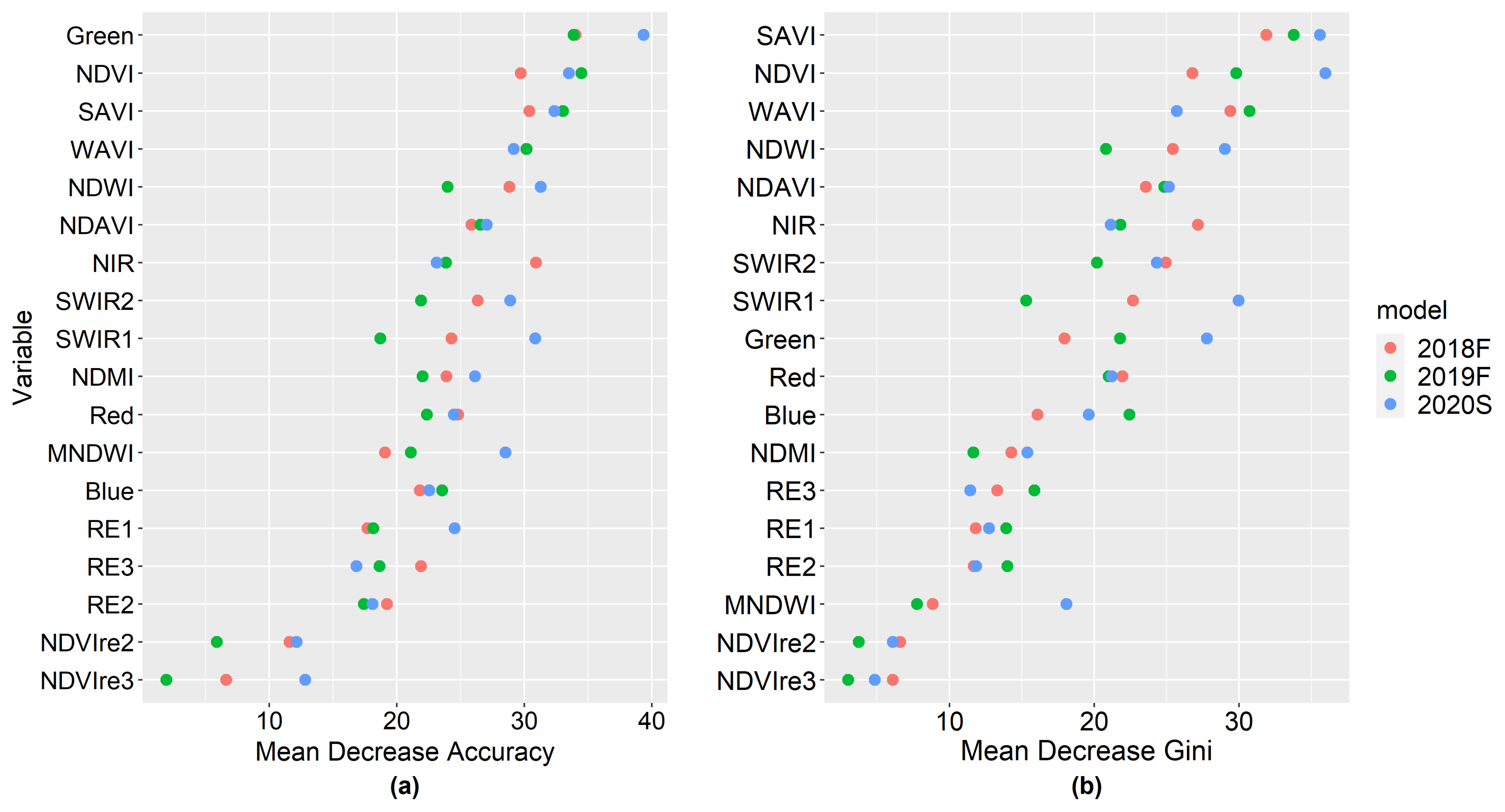
3.2. Sentinel-2 Forest Variable Importance

Figure 3 shows the random forest variable importance for Sentinel-2 models: variables are ordered by the mean decrease accuracy (MDA) considering all models. MDA and mean decrease gini (MDG) are common measures of variable importance for random forest models. Inputs with high MDA or MDG indicate high importance to the model; additional information on their computation and use can be found in [57,58]. Spectral indexes were consistently ranked with high importance, along with the green spectral reflectance band followed by SWIR and NIR spectral reflectance bands (Figure 3). High importance of spectral indexes has been previously identified in other aquatic vegetation classification studies targeting floating vegetation [17,25]. The NIR band contributes to the separation of different FAV covers and emergent vegetation while the SWIR bands are critical to differentiating emergent and FAV from water [14]. Although ranked lower than most other spectral bands in our models, the red edge bands had reasonably high mean average decrease values indicating they were valuable to model performance. The two red edge indexes, NDVIre2 and NDVIre3, were the least important in all models.

3.3. Sentinel-2 and AIS Genus-Level Map Comparison

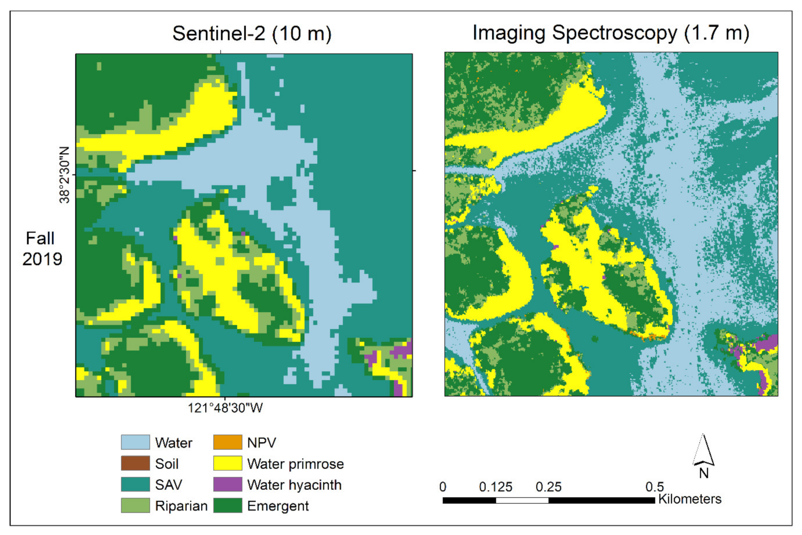
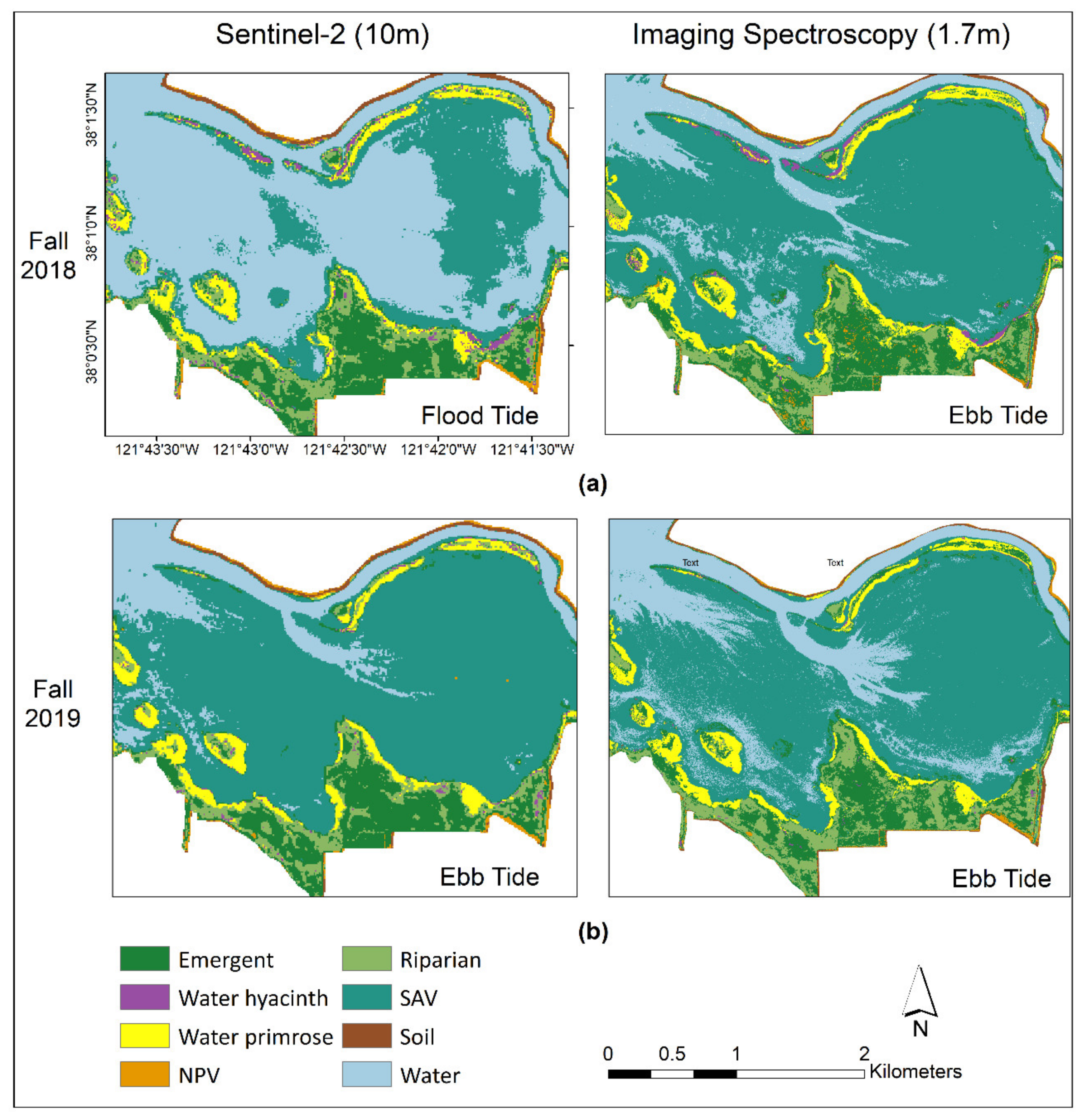
3.3.1. Visual Comparison in Two Sites

Classification results between the two sensors were visually similar for all three dates throughout much of the Delta, here we show this by comparing 2019 Fall Sentinel-2 and AIS maps of Ward Cut and Rhode Island in Figure 4. We chose to display these two sites because they contained all study classes and exhibited a range of different vegetation patch sizes and shapes. Generally good agreement between maps was observed at the FAV genus level between locations of larger water primrose (yellow) and water hyacinth patches (purple); however, there were some thinner water hyacinth patches present in AIS maps that were undetected at the coarser Sentinel-2 resolution (Figure 4a). The largest differences between the two maps resulted from EAV and riparian confusion and the detected SAV coverage relative to tidal stage during image acquisition (Table 2).

3.3.2. Percent Coverage Comparison

To characterize over- or underestimation of classes in Sentinel-2 maps relative to AIS maps, we calculated the percent area each class occupied in both maps and subtracted AIS percent area from that of Sentinel-2 in four key study sites and the Delta as a whole (

Table 6. Difference in percent coverage between Sentinel-2 and airborne imaging spectrometer (AIS) classification maps for 4 sub study areas and Delta wide. AIS percent coverage was subtracted from that of Sentinel-2; therefore, negative values indicate Sentinel-2 underestimation (blue), while positive values indicate Sentinel-2 overestimation (yellow) relative to AIS maps.

Date		Water Hyacinth	Water Primrose	EAV	Riparian	SAV	Water
2018F	Ward Cut	−0.2	−0.3	−2.9	2.8	0.7	−2.1
	Rhode Island	0.4	−6.5	−1.3	10.4	1.9	−5.2
	Big Break	0.2	−0.8	−2.2	1.8	−31.5	32.1
	Liberty	0	−0.5	−1.3	2.6	−2.2	2.7
	Delta	0.2	−0.6	−2.7	2	−5.8	−0.5
2019F	Ward Cut	−0.2	−0.2	2.3	−2.6	−0.4	−0.1
	Rhode Island	1.8	−1.9	−2.2	5.4	0.8	−2.1
	Big Break	0.3	0	0.1	−1.1	6.7	−6.2
	Liberty	0.2	−0.7	6.3	−6.8	7	−4.5
	Delta	−0.1	−0.3	4.1	−4.6	−2.4	0.1
2020S	Ward Cut	0.4	−1.9 *	2.5 *	1.2 *	−2.7	−1
	Rhode Island	1.1	−3.7 *	1.1 *	7.7 *	7.4	−12.7
	Big Break	0.3	0.6 *	−0.5 *	−0.4 *	−8	9.3
	Liberty	0	1.1 *	5.7 *	−3.1 *	7.8	−8.3
	Delta	0.4	−0.4 *	5.3 *	−3.3 *	−0.4	−6.3

* AIS emergent primrose class was not re-grouped as either primrose or emergent in Sentinel-2 maps.

). Thus, negative values in Table 6 indicate Sentinel-2 underestimation, while positive values indicate Sentinel-2 overestimation. Actual percent coverages are reported in Appendix A. We compared percent coverage rather than individual pixel agreement because the AIS maps have their own classification errors and reports to state agencies characterizing AIS mapping results primarily focus on percent coverage comparison across years. Similar to class accuracy, we only compared the five vegetation classes and open water.

Water hyacinth percent coverage was overestimated compared to AIS for all comparisons except Ward Cut in fall 2018 and 2019 and Delta wide in fall 2019; however, the difference for all these sites was quite small (0.1–0.2%). The largest differences in water hyacinth percent coverage were in Rhode Island (0.4–1.8%) and across the Delta in summer 2020 (0.4%). Rhode Island fall 2019 maps are displayed in Figure 4b and show good matchup between medium and large patch locations and extent, despite having the largest percent coverage difference compared to AIS. Orange non-photosynthetic vegetation (NPV) patches on the edge of islands in AIS maps are patches of floating NPV which cannot be detected by Sentinel-2 spatial or spectral resolution. Differences in SAV detection for both areas are likely due to image quality or differences in water height during acquisition, the latter is further discussed in Section 4.3.

Water primrose was underestimated relative to AIS in all locations except Big Break in fall 2019 (no difference), and Big Break and Liberty Island in summer 2020. Water primrose percent differences in summer 2020 were impacted by the additional emergent primrose class in AIS maps which was included to characterize areas of water primrose encroachment on emergent habitat [39]. Potential explanations for difference in water hyacinth and water primrose percent coverage are provided in the discussion.

Emergent and riparian vegetation had relatively high percent coverage differences between datasets and exhibited a less distinct pattern of over- or underestimation across years unlike the two FAV classes, although they appeared to be inversely related, likely due to their class confusion. The largest difference between maps was Sentinel-2 SAV underestimation and consequently, water overestimation in fall 2018 for Big Break (Table 6), which may be due to tidal height (Table 2).

4. Discussion

RS classification of multiple FAV classes is sparse in the published literature, especially in complex aquatic systems such as the Delta. Most previous works target only a single floating invasive species or classify at the community level and are conducted in areas with low spatial variability and large contiguous patches making it easier to separate FAV species from other neighboring aquatic vegetation [59,60,61]. Previous studies in the Delta rely on airborne imaging spectroscopy (AIS) to separate different FAV covers [14,17,39]. In order to determine if Sentinel-2 could be used to fill in AIS temporal gaps with acceptable detection of FAV at the genus level, we compared classification model accuracies (Table 5) and maps between the two datasets visually (e.g., Figure 4) and by difference percent class coverage (Table 6) and discuss dependence on patch size and within class variability relative to sensor spatial and spectral resolution and the influence of external factors such as tidal stage. We further compared differences for both summer and fall imagery to determine if Sentinel-2 maps could be created for multiple dates throughout the growing season, thereby enabling tracking of patch expansion and movement of these motile aquatic species.

4.1. Model Accuracies

Following a similar procedure to the near-operational AIS mapping in the Delta, we were able to achieve similar overall accuracies (OA) of 89–91% with Sentinel-2 compared to 90–92% of AIS while mapping the same classes—water hyacinth (species level), water primrose (genus level), SAV, EAV, and riparian vegetation at the community level, and open water, soil, and non-photosynthetic vegetation. Our overall Sentinel-2 accuracies were also comparable to other multispectral RS studies which target 4 macrophyte classes and open water 90% [61,62] (although neither target multiple FAV classes).

The average Sentinel-2 class accuracy statistics for our target FAV classes—water hyacinth (PA: 79%, UA: 91%) and water primrose (PA: 95%, UA: 85%) were lower or comparable with AIS water hyacinth (PA: 89%, UA: 90%) and water primrose (PA: 93%, UA: 93%). Our performance was also better than, or in line with, other Sentinel-2 studies targeting water hyacinth, which achieved user’s accuracies of 75–89% and producer’s accuracies 61–94% using random forest models [25,60]. To our knowledge, this is the first study to demonstrate water primrose mapping using multispectral satellite remote sensing; therefore, we are unable to compare class specific accuracies to other sites, but generally our accuracies were quite high.

The spatial resolution of the data relative to target patch size influenced the detection capability of the classifiers, and subsequent differences in percent coverage calculated from Sentinel 2. Generally, larger pixel sizes lead to poorer accuracy statistics, though the relationship is not linear; the effect of pixel size on accuracy is dependent on the heterogeneity of the landscape and the design and geolocational precision and accuracy of field data [63,64]. Spatial resampling Sentinel-2 bands of varying spatial resolution to 10 m may have further impacted the ability to detect small scale features. Nearest neighbor resampling is recommended to be both computationally efficient while best preserving pixel spectral information [65] and has been shown to be suitable for Sentinel-2 land cover classification [66]. More specialized downscaling algorithms could be explored in future research, although the effects of downscaling on classification accuracy are highly variable [67,68]. The pixel size influence on accuracy was minimized in this study through the field data collection and curation process, which paid special attention to patch size relative to the spatial resolution of the two RS datasets. Unfortunately, this same data design process may have possibly introduced lower quality training data into the models resulting in confusion between water hyacinth and water primrose and EAV and riparian vegetation. AIS observations indicate that water hyacinth patches are commonly interspersed with or surrounded by water primrose; therefore, patches labeled as majority water hyacinth in the field data may contain enough water primrose coverage to influence the spectral signature at the Sentinel-2 pixel size. EAV commonly forms narrow patches which are difficult to photo-interpret and observe in the field due to logistical challenges associated with access and plant density and height obscuring field observations. This poses an issue particularly for Sentinel-2 discrimination because at coarser spatial resolutions it becomes even more difficult to separate emergent vegetation from the riparian vegetation located directly behind it. It is recommended that future field data collection focus on building training datasets of large and heterogenous aquatic vegetation patches and better characterization of fractional cover and patch sizes relative to Sentinel-2 pixel size.

4.2. Percent Coverage of FAV Classes

Our Sentinel-2 maps matched well with AIS maps visually (Figure 4), but our areal comparison analysis indicated that S2 classifiers generally overestimated water hyacinth and underestimated water primrose area relative to AIS (Table 6). Infrequent classes with small patches, such as water hyacinth, are actually expected to be underestimated since small patches are likely to be undetected at coarser spatial resolutions—this was exhibited for certain patches, for example, the long and thin patch in Ward Cut was missed by S2 (Figure 4). However, under-detection of small and narrow water hyacinth patches was outweighed in percent coverage estimates because of S2 pixel size, confusion with riparian vegetation due to similar spectral signatures in multispectral space (Figure 5), and ‘sporadic’ misclassification likely due to other mixed pixels or within class spectral variability not accounted for in the training dataset. This confusion could be reduced with higher spectral resolution data, as it enables spectral unmixing of spectrally complex and similar classes [13,18]. However, even previous AIS studies in the Delta found some confusion between these classes [18]. These studies reduced misidentification of riparian vegetation as water hyacinth by creating a riparian mask based on spatial information regarding wetland and channel configuration derived from ancillary GIS layers and LiDAR data, which we recommend for future studies [18].

Water primrose coverage was likely underestimated due to Sentinel-2 mixed pixels at class boundaries exemplified in Figure 6, which shows patch edges that are more likely to be mixed with water or SAV classified as emergent or riparian vegetation in Sentinel-2 imagery. Such effects were more pronounced for water primrose patches than water hyacinth because water primrose shares a larger interface with other classes due to its dominance in the system. In recent years, water primrose has rapidly increased in abundance and distribution in the Delta, and several regions across the Delta have experienced marsh encroachment of water primrose, where water primrose has been “terrestrializing” and creeping up on top of emergent reeds [39]. The AIS summer 2020 maps labeled this as a separate class (“emergent primrose”), but Sentinel-2 does not have the spectral or spatial resolution required to do so. Instead, Sentinel-2 identifies the dominant class representing whichever vegetation is on top of the heterogeneous 3D structure, thereby resulting in percent coverage differences that are not directly related to misclassification.

4.3. Impact of Environmental Conditions: Tidal Stage

Other large mismatches in visual and percent area assessments occurred for the SAV and water classes; these differences are likely explained by differences in tidal stage during image acquisition rather than Sentinel-2 misclassification. Figure 7 explores the impact of tide-stage mismatch between datasets more extensively by comparing a good tidal match-up date (fall 2019) with one of lesser quality (fall 2018). Fall 2018 Sentinel-2 acquisition occurred during a flood tide, which impedes detection of full SAV extent. Fall 2019 Sentinel-2 acquisition occurred at a low tide and showed a much closer match-up between Sentinel-2 and AIS maps. This indicates that SAV is detectable with Sentinel-2, but images should be selected at low tide to reduce the impacts of water height and increased turbidity, which inhibit detection of the full extent for SAV coverage. Such an approach would mirror the current operations for AIS-based SAV mapping, which only acquires data during periods of low tide and during times of the day that avoid effects from sun glint [13,39]. Tidal stage did not strongly impact FAV mapping because the leaves are above the water column hence spectral reflectance is not affected by tidal stage. Both water hyacinth and water primrose exhibited a good visual match and smaller quantitative differences, as listed in Table 6.

4.4. Sentinel-2 Characteristics That Enable Differentiation between FAV Classes and the Neighboring Vegetation

The detection of water hyacinth and water primrose in this spatially complex system of wetlands was possible due to the 10–20 m pixel size of Sentinel-2 images and the moderate spectral resolution. While some previous multi-spectral RS studies targeting water hyacinth detection have successfully used Landsat (30 m pixels; 7 bands) [24], these studies occurred in simpler systems with fewer target species. Thamaga and Dube (2018b) compared the performance of Landsat and Sentinel-2 and determined that Sentinel-2 resulted in higher class accuracies. In an environment as spatially complex as the Delta, the 10 m spatial resolution of Sentinel-2 supports water primrose and water hyacinth detection because these vegetation patches are generally small (~40–60 m) wide with few large patches (90–100 m). Large patches would be contained within a single 30 m pixel, but smaller patches would not.

Spectral resolution and range also play important roles in FAV separation. Although the three Sentinel-2 red-edge bands were not ranked as high as several spectral indexes or spectral bands in Sentinel-2 RF model variable importance, the mean decrease accuracy values (~20%) suggest that the red edge bands still played an important role in class discrimination. The importance of the red edge bands to aquatic vegetation classification has been demonstrated in other studies [25,69]. These works, like ours, determined that spectral indexes and other VSWIR spectral bands are more important to classification accuracy than red edge bands, but this does not negate the usefulness of these additional Sentinel-2 bands. However, red edge indices were consistently among the least important variables, their importance has varied in other aquatic vegetation classification studies [69,70]. Additional testing is recommended to determine if these red edge indexes could be excluded in future models. Spectral range is also an important consideration. The SWIR region, and spectral indexes calculated with SWIR bands were important for RF model performance. Previous works have also documented the importance in the SWIR region for discriminating aquatic vegetation from water [18,71].

5. Conclusions

Analysis of Sentinel-2 classifications maps demonstrated that two types of invasive floating aquatic vegetation, water hyacinth and water primrose, can be distinguished in heterogeneous wetlands during summer and fall. Our results indicated that Sentinel-2 imagery can supplement AIS mapping efforts by filling temporal gaps and enabling studying of annual and intra-annual changes in FAV community composition as a response to environmental or anthropogenic disturbance events. Extensive time series will, in particular, enhance the understanding of invasion processes. Future research should investigate differences in spring and winter and incorporate a riparian vegetation mask to reduce misclassification of floating vegetation. Further, the near-operational pipeline developed during this study will lead to an operational mapping pipeline for generating wetland vegetation maps for California agencies that enable new methods of management and monitoring to identify where aquatic invasive species control is effective.

References

1. Gordon, D.R. Effects of invasive, non-indigenous plant species on ecosystem processes: Lessons from florida. Conserv. Biol. 975 Ecol. Appl. 1998, 8, 975–989. [Google Scholar] [CrossRef]
2. Scheffer, M.; Szabo, S.; Gragnani, A.; Van Nes, E.H.; Rinaldi, S.; Kautsky, N.; Norberg, J.; Roijackers, R.M.M.; Franken, R.J.M. Floating Plant Dominance as a Stable State. Proc. Natl. Acad. Sci. USA 2003, 100, 4040–4045. [Google Scholar] [CrossRef] [PubMed] [Green Version]
3. Dukes, J.S.; Mooney, H.A. Disruption of Ecosystem Processes in Western North America by Invasive Species. Rev. Chil. Hist. Nat. 2004, 77, 411–437. [Google Scholar] [CrossRef]
4. O’Farrell, I.; De Tezanos Pinto, P.; Rodríguez, P.L.; Chaparro, G.; Pizarro, H.N. Experimental Evidence of the Dynamic Effect of Free-Floating Plants on Phytoplankton Ecology. Freshw. Biol. 2009, 54, 363–375. [Google Scholar] [CrossRef]
5. Ongore, C.O.; Aura, C.M.; Ogari, Z.; Njiru, J.M.; Nyamweya, C.S. Spatial-Temporal Dynamics of Water Hyacinth, Eichhornia crassipes (Mart.) and Other Macrophytes and Their Impact on Fisheries in Lake Victoria, Kenya. J. Great Lakes Res. 2018, 44, 1273–1280. [Google Scholar] [CrossRef]
6. Pimentel, D.; Zuniga, R.; Morrison, D. Update on the Environmental and Economic Costs Associated with Alien-Invasive Species in the United States. Ecol. Econ. 2005, 52, 273–288. [Google Scholar] [CrossRef]
7. Thouvenot, L.; Haury, J.; Thiebaut, G. A Success Story: Water Primroses, Aquatic Plant Pests. Aquat. Conserv. Mar. Freshw. Ecosyst. 2013, 23, 790–803. [Google Scholar] [CrossRef]
8. Thamaga, K.H.; Dube, T. Remote Sensing of Invasive Water Hyacinth (Eichhornia crassipes): A Review on Applications and Challenges. Remote Sens. Appl. Soc. Environ. 2018, 10, 36–46. [Google Scholar] [CrossRef]
9. Adam, E.; Mutanga, O.; Rugege, D. Multispectral and Hyperspectral Remote Sensing for Identification and Mapping of Wetland Vegetation: A Review. Wetl. Ecol. Manag. 2010, 18, 281–296. [Google Scholar] [CrossRef]
10. Gallant, A.L. The Challenges of Remote Monitoring of Wetlands. Remote Sens. 2015, 7, 10938–10950. [Google Scholar] [CrossRef] [Green Version]
11. Guo, M.; Li, J.; Sheng, C.; Xu, J.; Wu, L. A Review of Wetland Remote Sensing. Sensors 2017, 17, 777. [Google Scholar] [CrossRef] [Green Version]
12. Everitt, J.H.; Yang, C.; Summy, K.R.; Owens, C.S.; Glomski, L.M.; Smart, R.M. Using in Situ Hyperspectral Reflectance Data to Distinguish Nine Aquatic Plant Species. Geocarto Int. 2011, 26, 459–473. [Google Scholar] [CrossRef]
13. Hestir, E.L.; Khanna, S.; Andrew, M.E.; Santos, M.J.; Viers, J.H.; Greenberg, J.A.; Rajapakse, S.S.; Ustin, S.L. Identification of Invasive Vegetation Using Hyperspectral Remote Sensing in the California Delta Ecosystem. Remote Sens. Environ. 2008, 112, 4034–4047. [Google Scholar] [CrossRef]
14. Khanna, S.; Santos, M.J.; Ustin, S.L.; Haverkamp, P.J. An Integrated Approach to a Biophysiologically Based Classification of Floating Aquatic Macrophytes. Int. J. Remote Sens. 2011, 32, 1067–1094. [Google Scholar] [CrossRef]
15. Santos, M.J.; Hestir, E.L.; Khanna, S.; Ustin, S.L. Image Spectroscopy and Stable Isotopes Elucidate Functional Dissimilarity between Native and Nonnative Plant Species in the Aquatic Environment. New Phytol. 2012, 193, 683–695. [Google Scholar] [CrossRef]
16. Schmidt, K.S.; Skidmore, A.K. Spectral Discrimination of Vegetation Types in a Coastal Wetland. Remote Sens. Environ. 2003, 85, 92–108. [Google Scholar] [CrossRef]
17. Bolch, E.A.; Hestir, E.L.; Khanna, S. Performance and Feasibility of Drone-Mounted Imaging Spectroscopy for Invasive Aquatic Vegetation Detection. Remote Sens. 2021, 13, 582. [Google Scholar] [CrossRef]
18. Khanna, S.; Santos, M.J.; Hestir, E.L.; Ustin, S.L. Plant Community Dynamics Relative to the Changing Distribution of a Highly Invasive Species, Eichhornia crassipes: A Remote Sensing Perspective. Biol. Invasions 2012, 14, 717–733. [Google Scholar] [CrossRef]
19. Kleinschroth, F.; Winton, R.S.; Calamita, E.; Niggemann, F.; Botter, M.; Wehrli, B.; Ghazoul, J. Living with Floating Vegetation Invasions. Ambio 2021, 50, 125–137. [Google Scholar] [CrossRef]
20. Drusch, M.; Del Bello, U.; Carlier, S.; Colin, O.; Fernandez, V.; Gascon, F.; Hoersch, B.; Isola, C.; Laberinti, P.; Martimort, P. Sentinel-2: ESA’s Optical High-Resolution Mission for GMES Operational Services. Remote Sens. Environ. 2012, 120, 25–36. [Google Scholar] [CrossRef]
21. Dong, D.; Wang, C.; Yan, J.; He, Q.; Zeng, J.; Wei, Z. Combing Sentinel-1 and Sentinel-2 Image Time Series for Invasive Spartina Alterniflora Mapping on Google Earth Engine: A Case Study in Zhangjiang Estuary. J. Appl. Remote Sens. 2020, 14, 1–18. [Google Scholar] [CrossRef]
22. Gong, Z.; Zhang, C.; Zhang, L.; Bai, J.; Zhou, D. Assessing Spatiotemporal Characteristics of Native and Invasive Species with Multi-Temporal Remote Sensing Images in the Yellow River Delta, China. L. Degrad. Dev. 2021, 32, 1338–1352. [Google Scholar] [CrossRef]
23. Dersseh, M.G.; Tilahun, S.A.; Worqlul, A.W.; Moges, M.A.; Abebe, W.B.; Mhiret, D.A.; Melesse, A.M. Spatial and Temporal Dynamics of Water Hyacinth and Its Linkage with Lake-Level Fluctuation: Lake Tana, a Sub-Humid Region of the Ethiopian Highlands. Water 2020, 12, 1435. [Google Scholar] [CrossRef]
24. Singh, G.; Reynolds, C.; Byrne, M.; Rosman, B. A Remote Sensing Method to Monitor Water, Aquatic Vegetation, and Invasive Water Hyacinth at National Extents. Remote Sens. 2020, 12, 4021. [Google Scholar] [CrossRef]
25. Thamaga, K.H.; Dube, T. Testing Two Methods for Mapping Water Hyacinth (Eichhornia crassipes) in the Greater Letaba River System, South Africa: Discrimination and Mapping Potential of the Polar-Orbiting Sentinel-2 MSI and Landsat 8 OLI Sensors. Int. J. Remote Sens. 2018, 39, 8041–8059. [Google Scholar] [CrossRef]
26. Khanna, S.; Ustin, S.L.; Hestir, E.L.; Santos, M.J.; Andrew, M.; Lay, M.; Tuil, J.; Bellvert, J.; Greenberg, J.; Shapiro, K.D.; et al. The Sacramento-San Joaquin Delta Genus and Community Level Classification Maps Derived. Airborne Spectroscopy Data. 2022. Available online: https://search-dev.test.dataone.org/view/doi%3A10.5063%2FF1K9360F (accessed on 3 May 2022).
27. Jetter, K.M.; Nes, K.; Tahoe, L. The Cost to Manage Invasive Aquatic Weeds in the California Bay-Delta. ARE Updat. 2018, 21, 9–11. [Google Scholar]
28. Rejmánková, E. Ecology of Creeping Macrophytes with Special Reference to Ludwigia peploides (H.B.K.) Raven. Aquat. Bot. 1992, 43, 283–299. [Google Scholar] [CrossRef]
29. Penfound, W.T.; Earle, T.T. The Biology of the Water Hyacinth. Ecol. Monogr. 1948, 18, 447–472. [Google Scholar] [CrossRef]
30. Grewell, B.J.; Gillard, M.B.; Futrell, C.J.; Castillo, J.M. Seedling Emergence from Seed Banks in Ludwigia hexapetala-Invaded Wetlands: Implications for Restoration. Plants 2019, 8, 451. [Google Scholar] [CrossRef] [Green Version]
31. Malik, A. Environmental Challenge Vis a Vis Opportunity: The Case of Water Hyacinth. Environ. Int. 2007, 33, 122–138. [Google Scholar] [CrossRef]
32. Ta, J.; Anderson, L.W.J.; Christman, M.A.; Khanna, S.; Kratville, D.; Madsen, J.D.; Moran, P.J.; Viers, J.H.; Ta, J.; Anderson, L.W.J.; et al. Invasive Aquatic Vegetation Management in the Sacramento-San Joaquin River Delta: Status and Recommendations. San Fr. Estuary Watershed Sci. 2017, 15, 5. [Google Scholar] [CrossRef] [Green Version]
33. Cohen, A.N.; Carlton, J.T. Accelerating Invasion Rate in a Highly Invaded Estuary. Science 1998, 279, 555–558. [Google Scholar] [CrossRef] [PubMed] [Green Version]
34. DBW. Aquatic Invasive Plant Control Program 2019 Annual Monitoring Report; California Department of Boating and Waterways: Sacramento, CA, USA, 2019. [Google Scholar]
35. Khanna, S.; Acuna, S.; Contreras, D.; Griffiths, W.K.; Lesmeister, S.; Reyes, R.C.; Schreier, B.; Wu, B.J. Invasive Aquatic Vegetation Impacts on Delta Operations, Monitoring, and Ecosystem and Human Health. IEP Newsl. 2019, 36, 8–18. [Google Scholar]
36. Hestir, E.L.; Greenberg, J.A.; Ustin, S.L. Classification Trees for Aquatic Vegetation Community Prediction from Imaging Spectroscopy. IEEE J. Sel. Top. Appl. Earth Obs. Remote Sens. 2012, 5, 1572–1584. [Google Scholar] [CrossRef]
37. Ustin, S.L.; Khanna, S.; Lay, M. Remote Sensing of the Sacramento-San Joaquin Delta to Enhance Mapping for Invasive and Native Aquatic Plant Species; University of California, Davis. Report to The Delta Stewardship Council; University of California Davis: Davis, CA, USA, 2021. [Google Scholar]
38. Ranghetti, L.; Boschetti, M.; Nutini, F.; Busetto, L. “Sen2r”: An R Toolbox for Automatically Downloading and Preprocessing Sentinel-2 Satellite Data. Comput. Geosci. 2020, 139, 104473. [Google Scholar] [CrossRef]
39. Khanna, S.; Santos, M.J.; Boyer, J.D.; Shapiro, K.D.; Bellvert, J.; Ustin, S.L. Water Primrose Invasion Changes Successional Pathways in an Estuarine Ecosystem. Ecosphere 2018, 9, e02418. [Google Scholar] [CrossRef]
40. Rosenfield, G.H.; Fitzpatrick-Lins, K. A Coefficient of Agreement as a Measure of Thematic Classification Accuracy. Photogramm. Eng. Remote Sens. 1986, 52, 223–227. [Google Scholar]
41. Story, M.; Congalton, R.G. Accuracy Assessment: A User’s Perspective. Photogramm. Eng. Remote Sens. 1986, 52, 397–399. [Google Scholar]
42. Berhane, T.M.; Lane, C.R.; Wu, Q.; Autrey, B.C.; Anenkhonov, O.A.; Chepinoga, V.V.; Liu, H. Decision-Tree, Rule-Based, and Random Forest Classification of High-Resolution Multispectral Imagery for Wetland Mapping and Inventory. Remote Sens. 2018, 10, 580. [Google Scholar] [CrossRef] [Green Version]
43. Magidi, J.; Nhamo, L.; Mpandeli, S.; Mabhaudhi, T. Application of the Random Forest Classifier to Map Irrigated Areas Using Google Earth Engine. Remote Sens. 2021, 13, 876. [Google Scholar] [CrossRef]
44. Mahdianpari, M.; Salehi, B.; Mohammadimanesh, F.; Motagh, M. Random Forest Wetland Classification Using ALOS-2 L-Band, RADARSAT-2 C-Band, and TerraSAR-X Imagery. ISPRS J. Photogramm. Remote Sens. 2017, 130, 13–31. [Google Scholar] [CrossRef]
45. Breiman, L. Random Forests. Mach. Learn. 2001, 45, 5–32. [Google Scholar] [CrossRef] [Green Version]
46. Liaw, A.; Wiener, M. Classification and Regression by RandomForest. R News 2002, 2, 18–22. [Google Scholar]
47. Kuhn, M. Building Predictive Models in R Using the Caret Package. J. Stat. Softw. 2008, 28, 1–26. [Google Scholar] [CrossRef] [Green Version]
48. Rouse, J.W.; Haas, R.H.; Schell, J.A.; Deering, D.W. Monitoring Vegetation Systems in the Great Plains with ERTS. NASA Spec. Publ. 1974, 351, 309. [Google Scholar]
49. Villa, P.; Laini, A.; Bresciani, M.; Bolpagni, R. A Remote Sensing Approach to Monitor the Conservation Status of Lacustrine Phragmites australis Beds. Wetl. Ecol. Manag. 2013, 21, 399–416. [Google Scholar] [CrossRef]
50. Villa, P.; Mousivand, A.; Bresciani, M. Aquatic Vegetation Indices Assessment through Radiative Transfer Modeling and Linear Mixture Simulation. Int. J. Appl. Earth Obs. Geoinf. 2014, 30, 113–127. [Google Scholar] [CrossRef]
51. Huete, A.R. A Soil-Adjusted Vegetation Index (SAVI). Remote Sens. Environ. 1988, 25, 295–309. [Google Scholar] [CrossRef]
52. Gitelson, A.; Merzlyak, M.N. Spectral Reflectance Changes Associated with Autumn Senescence of Aesculus Hippocastanum L. and Acer Platanoides L. Leaves. Spectral Features and Relation to Chlorophyll Estimation. J. Plant Physiol. 1994, 143, 286–292. [Google Scholar] [CrossRef]
53. Fernández-Manso, A.; Fernández-Manso, O.; Quintano, C. SENTINEL-2A Red-Edge Spectral Indices Suitability for Discriminating Burn Severity. Int. J. Appl. Earth Obs. Geoinf. 2016, 50, 170–175. [Google Scholar] [CrossRef]
54. McFeeters, S.K. The Use of the Normalized Difference Water Index (NDWI) in the Delineation of Open Water Features. Int. J. Remote Sens. 1996, 17, 1425–1432. [Google Scholar] [CrossRef]
55. Gao, B.C. NDWI—A Normalized Difference Water Index for Remote Sensing of Vegetation Liquid Water from Space. Remote Sens. Environ. 1996, 58, 257–266. [Google Scholar] [CrossRef]
56. Xu, H. Modification of Normalised Difference Water Index (NDWI) to Enhance Open Water Features in Remotely Sensed Imagery. Int. J. Remote Sens. 2006, 27, 3025–3033. [Google Scholar] [CrossRef]
57. Cutler, D.R.; Edwards, T.C.; Beard, K.H.; Cutler, A.; Hess, K.T.; Gibson, J.; Lawler, J.J. Random forests for classification in ecology. Ecology 2007, 88, 2783–2792. [Google Scholar] [CrossRef]
58. Han, H.; Guo, X.; Yu, H. Variable Selection Using Mean Decrease Accuracy and Mean Decrease Gini Based on Random Forest. In Proceedings of the 2016 7th IEEE International Conference on Software Engineering and Service Science (ICSESS), Beijing, China, 26–28 August 2016; pp. 219–224. [Google Scholar] [CrossRef]
59. Dogliotti, A.I.; Gossn, J.I.; Vanhellemont, Q.; Ruddick, K.G. Detecting and Quantifying a Massive Invasion of Floating Aquatic Plants in the Río de La Plata Turbid Waters Using High Spatial Resolution Ocean Color Imagery. Remote Sens. 2018, 10, 1140. [Google Scholar] [CrossRef] [Green Version]
60. Thamaga, K.H.; Dube, T. Understanding Seasonal Dynamics of Invasive Water Hyacinth (Eichhornia crassipes) in the Greater Letaba River System Using Sentinel-2 Satellite Data. GISci. Remote Sens. 2019, 56, 1355–1377. [Google Scholar] [CrossRef]
61. Villa, P.; Bresciani, M.; Bolpagni, R.; Pinardi, M.; Giardino, C. A Rule-Based Approach for Mapping Macrophyte Communities Using Multi-Temporal Aquatic Vegetation Indices. Remote Sens. Environ. 2015, 171, 218–233. [Google Scholar] [CrossRef] [Green Version]
62. Wang, L.; Dronova, I.; Gong, P.; Yang, W.; Li, Y.; Liu, Q. A New Time Series Vegetation-Water Index of Phenological-Hydrological Trait across Species and Functional Types for Poyang Lake Wetland Ecosystem. Remote Sens. Environ. 2012, 125, 49–63. [Google Scholar] [CrossRef]
63. Frazier, A.E. Landscape Heterogeneity and Scale Considerations for Super-Resolution Mapping. Int. J. Remote Sens. 2015, 36, 2395–2408. [Google Scholar] [CrossRef]
64. Knight, J.F.; Lunetta, R.S. An Experimental Assessment of Minimum Mapping Unit Size. IEEE Trans. Geosci. Remote Sens. 2003, 41, 2132–2134. [Google Scholar] [CrossRef]
65. Roy, D.P.; Li, J.; Zhang, H.K.; Yan, L. Best Practices for the Reprojection and Resampling of Sentinel-2 Multi Spectral Instrument Level 1C Data. Remote Sens. Lett. 2016, 7, 1023–1032. [Google Scholar] [CrossRef]
66. Zheng, H.; Du, P.; Chen, J.; Xia, J.; Li, E.; Xu, Z.; Li, X.; Yokoya, N. Performance Evaluation of Downscaling Sentinel-2 Imagery for Land Use and Land Cover Classification by Spectral-Spatial Features. Remote Sens. 2017, 9, 1274. [Google Scholar] [CrossRef] [Green Version]
67. Morrison, B.D.; Heath, K.; Greenberg, J.A. Spatial Scale Affects Novel and Disappeared Climate Change Projections in Alaska. Ecol. Evol. 2019, 9, 12026–12044. [Google Scholar] [CrossRef] [PubMed]
68. Vanderbilt, V.C.; Khanna, S.; Ustin, S.L. Impact of Pixel Size on Mapping Surface Water in Subsolar Imagery. Remote Sens. Environ. 2007, 109, 1–9. [Google Scholar] [CrossRef]
69. Tian, Y.; Jia, M.; Wang, Z.; Mao, D.; Du, B.; Wang, C. Monitoring Invasion Process of Spartina Alterniflora by Seasonal Sentinel-2 Imagery and an Object-Based Random Forest Classification. Remote Sens. 2020, 12, 1383. [Google Scholar] [CrossRef]
70. Amani, M.; Salehi, B.; Mahdavi, S.; Brisco, B. Spectral Analysis of Wetlands Using Multi-Source Optical Satellite Imagery. ISPRS J. Photogramm. Remote Sens. 2018, 144, 119–136. [Google Scholar] [CrossRef]
71. Hestir, E.L.; Brando, V.E.; Bresciani, M.; Giardino, C.; Matta, E.; Villa, P.; Dekker, A.G. Measuring Freshwater Aquatic Ecosystems: The Need for a Hyperspectral Global Mapping Satellite Mission. Remote Sens. Environ. 2015, 167, 181–195. [Google Scholar] [CrossRef] [Green Version]
Figure 1. (A) Field photos of vegetation classes and list of species in each vegetation community type. (B) Mean spectral signatures for 2019 Sentinel-2 training data; shading represents 95% confidence interval. (C) Mean spectral signatures for 2019 AIS training data; shading represents 95% confidence interval. Data come from the HyMap sensor described in Section 2.3. See [32] for more in-depth descriptions of targeted invasive aquatic vegetation.
Remotesensing 14 03013 g001
Figure 2. Map of the Delta sub-study areas. RGB images were created using imaging spectroscopy acquisitions.
Remotesensing 14 03013 g002
Figure 3. Variable importance for Sentinel-2 random forest models for each match-up date, (a) Mean Decrease Accuracy and (b) Mean Decrease Gini. Variables are ordered by average decrease across all three models. Spectral indices consistently rank high in importance across all three model dates.
Remotesensing 14 03013 g003
Figure 4. (a) Ward Cut and (b) Rhode Island comparison between 2019 Sentinel-2 and imaging spectrometer maps. The comparison shows good agreement at the FAV genus level between locations of larger water primrose (yellow) and water hyacinth patches (purple).
Remotesensing 14 03013 g004
Figure 5. Spectral response of a riparian vegetation pixel that was misclassified as water hyacinth and a water hyacinth pixel.
Remotesensing 14 03013 g005
Figure 6. Comparison of the impact of limited spatial resolution in Sentinel-2 data using water primrose patches. Coarse pixel resolution is more likely to cause misclassification at class boundaries due to pixel mixing.
Remotesensing 14 03013 g006
Figure 7. Tidal stage comparison for fall match-ups at Big Break: (a) fall 2018 and (b) fall 2019. Fall 2018 Sentinel-2 acquisition occurred during a flood tide which impedes detection of full SAV extent. Fall 2019 Sentinel-2 acquisition occurred at a low tide and showed a much closer match-up between Sentinel-2 and imaging spectrometer maps.
Remotesensing 14 03013 g007