Article

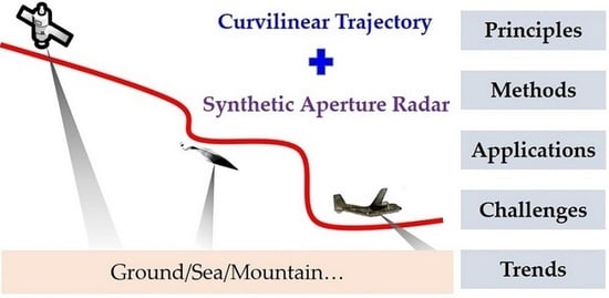
Curvilinear Flight Synthetic Aperture Radar (CF-SAR): Principles, Methods, Applications, Challenges and Trends

1
Chongqing Key Laboratory of Space Information Network and Intelligent Information Fusion, School of Microelectronics and Communication Engineering, Chongqing University, Chongqing 400044, China
2
National Laboratory of Radar Signal Processing, Xidian University, Xi’an 710071, China
3
College of Communication and Information Engineering, Xi’an University of Science and Technology, Xi’an 710054, China
4
State Key Lab of Millimeter Waves, School of Information Science and Engineering, Southeast University, Nanjing 210096, China
*
Author to whom correspondence should be addressed.
Remote Sens. 2022, 14(13), 2983; https://doi.org/10.3390/rs14132983
Submission received: 21 May 2022 / Revised: 15 June 2022 / Accepted: 20 June 2022 / Published: 22 June 2022

Abstract

:
The research into curvilinear flight synthetic aperture radar (CF-SAR) is the inevitable result of the comprehensive practicality of SAR. The flight path of the SAR platform in real applications, which is highly nonlinear or curvy due to three-dimensional velocity and acceleration, cannot be described by the traditional uniform linear motion model. New mathematical models, signal characteristics, imaging algorithms, and system design criteria must be proposed and investigated for CF-SAR. This paper provides a comprehensive overview of CF-SAR. Firstly, the basic concept, unified model, and general signal characteristics of CF-SAR are defined, derived, and analyzed, respectively. Additionally, the advantages and drawbacks of current methodologies are reviewed. Discussions on the CF-SAR’s applications are presented from the perspective of typical platforms, new configurations, and advanced technologies, which are suitable means to fulfill the increasing user requirements. Finally, the challenges faced by CF-SAR are summarized, and some future trends for the study of CF-SAR are explored. Hopefully, this paper will serve as a reference for SAR researchers/engineers and stimulate the future development and actual application of CF-SAR.

Graphical Abstract

1. Introduction

With the capability to obtain high-resolution microwave images of the observed scenarios regardless of meteorological and solar illumination conditions, synthetic aperture radar (SAR) has entered a golden age in remote sensing applications [1]. Generally, the high range resolution of SAR is obtained by performing pulse compression on the transmitted large-timewidth large-bandwidth modulation signal, such as the widely used linear frequency modulation signal, while the high azimuth resolution of SAR is obtained by performing match filtering on the virtual aperture synthesized by the real antennas at different positions. Differing from real-aperture radars, virtual array synthesis technology is the most significant feature of SAR, and its purpose is to break through the inverse limitation of real antennas to the resolution capability of conventional radars.
SAR has realized the transformation from one-dimensional (e.g., range, angle) rough processing to multi-dimensional (e.g., range–azimuth, range–Doppler) fine processing. Most of the early studies assumed that the virtual array of SAR was synthesized by using an ideal uniform linear trajectory of the real radar antenna [2]. In order to help the reader to distinguish this concept, this paper calls it conventional SAR (Conv-SAR). In fact, as sketched in Figure 1, the SAR platform usually moves in a curvilinear trajectory due to the influence of three-dimensional (3D) velocity or acceleration, such as atmospheric turbulence (e.g., helicopters), terrain evasion (e.g., unmanned aerial vehicles), maneuvering responses (e.g., hypersonic vehicle), orbital motion (e.g., satellites) and so on. The emergence of curvilinear flight SAR (CF-SAR) is the inevitable result of the comprehensive practicality of SAR.
Differing from the non-uniform linear motion of Conv-SAR caused by unintentional motion error [3], CF-SAR realizes the flexible control of the platform and fulfills different application requirements through intentional non-uniform motion, such as accelerated motion and widely concerned circular motion [4], etc. The non-uniform motion makes CF-SAR more suitable for the actual detection environment due to two reasons:
Highly adaptable to detection geometries. Taking complex application scenarios, such as mountain or urban surveying, as an example, Conv-SAR has to abandon imaging quality in exchange for a safe working environment. This is because the imaging geometry of Conv-SAR no longer meets the imaging requirements when performing terrain avoidance to obtain a safe path. However, the emergence of CF-SAR forces the detection geometry boundary of Conv-SAR to no longer be restricted to the condition of uniform linear virtual synthetic aperture. In other words, by effectively dealing with the nonlinear or non-uniform sampling data introduced by the curve trajectory, CF-SAR ensures the imaging performance and output rate under different detection geometries.
In-depth utilization of detection capabilities. Taking the selection of imaging area as an example, Conv-SAR has a forward-looking blind zone [5]. However, CF-SAR can solve the problem of forward-looking imaging through the autonomous adjustment of radar trajectory and arbitrary control of beam steering, which maximize the technical advantages of SAR. In other words, the nonlinear motion of the SAR platform can provide more degrees of freedom to explore the detection capabilities of SAR. As a special case of CF-SAR, the 3D imaging of the circular SAR [6] also demonstrates that CF-SAR can deeply utilize the detection ability of SAR. Similarly, a timely and rapid revisit of CF-SAR also provides a prerequisite for the SAR moving target indication capability.
With the abovementioned advantages, CF-SAR has unique application value and development potential to cope with various requirements in actual detection tasks. A lot of research has been conducted on the theoretical analysis and algorithm design of CF-SAR, and some actual CF-SAR system demos have also been developed. However, a thorough summary of the current technique status and discussions about future trends is lacking in the existing literature. By providing a comprehensive survey of the CF-SAR technique, this paper can serve as a reference for the future development and actual application of CF-SAR.
This paper is structured as follows. Section 2 introduces the principles of CF-SAR, and the basic concept, unified model, and general signal characteristics of CF-SAR are defined, derived, and analyzed, respectively. Then, a comprehensive literature review of the advantages and drawbacks of current state-of-the-art methodologies is presented in Section 3. In Section 4, discussions on the CF-SAR’s applications are presented from three perspectives, which are suitable means for fulfilling the increasing user requirements. Finally, Section 5 outlines the challenges faced by CF-SAR, and some future trends for the study of CF-SAR are explored, and the conclusions of this paper are summarized in Section 6.

2. Principle of CF-SAR

2.1. Basic Concept

Generally, all SARs that perform non-uniform linear motion can be attributed to CF-SAR. However, in this paper, from a narrow perspective, CF-SAR refers to the SAR moving with 3D velocity and 3D acceleration [7]. It should be noted that ‘CF’ is a description of the SAR movement status, not a classification of radar platform type. In other words, CF-SAR is an inevitable product of the full application of Conv-SAR.
Similar to Conv-SAR, CF-SAR can also be classified by different types such as platform, geometry configuration, antenna, imaging mode, etc., as shown in Figure 2, and this classification is summarized based on the existing conventional classification. With the development of SAR, the categories will be more varied.

2.2. Unified Model

A unified signal model is essential to the design of an SAR system and signal processing algorithms. The key problem in modeling is selecting a suitable coordinate system to determine the imaging geometry. In our recent research [8], an accurate model is derived based on the inertial navigation system (INS) data in the navigation coordinate system. However, for intuitive analysis and understanding, the geometry of monostatic CF-SAR is introduced in a Cartesian coordinate system, as shown in Figure 3.
Unlike the Conv-SAR, the flight path of CF-SAR is not straight due to accelerations. We set P as the reference position at the aperture center moment (ACM), and C as an arbitrary point target in the interested area. The instantaneous slant range between the sensor and C can be derived as:
R c η = R 0 V V t a r η 1 2 A A t a r η 2
where R 0 denotes the antenna position vectors from P to C at ACM, and V t a r and V are the velocity vectors of target and CF-SAR at ACM, respectively. A t a r and A represent the acceleration vectors of target and CF-SAR at ACM, respectively, and η is the slow-time. It is noted that two aspects are focused on in our CF-SAR geometry: (1) for high-orbit spaceborne CF-SAR, the Doppler influence caused by the rotation of the Earth cannot be ignored [9], which means that target cannot be considered as static, differing from Conv-SAR; (2) in addition to imaging stationary scenes, one of the most important applications of SAR is moving target indication. The stationary targets can be regarded as special cases where the moving target has no moving state, i.e., the speed, acceleration, and high-order acceleration are all zero. Then, for static and moving targets with the same initial position, their range histories can be modeled uniformly in Equation (1).
For CF-SAR with different modes, including stripmap, spotlight, sliding spotlight, and TOPS modes, etc., the main differences corresponding to the signal pattern between them depend on the beam steering and the position of the rotation center [10]. According to Equation (1), the echo signal of CF-SAR in Figure 3 after down-conversion can be expressed as follows:
s t , η = i σ i w r t 2 R i η / c T p w a η η i T a exp j 2 π f c 2 R i η c + j 2 π ϕ p t 2 R i η c
where w r t and w a η denote the range and azimuth window function, respectively, t is the fast-time variable, T p and T a are the pulse width and synthetic aperture time, respectively, f c is the carrier frequency of the transmitted signal, c is the speed of the light, σ i , η i and R i η represent the complex amplitude, ACM, and instantaneous slant range of the i-th point target, respectively, and ϕ p t represents the signal modulation phase. From the perspective of SAR signal processing algorithm design, there are some remarks for the proposed unified signal model in Equation (2):
Remark 1.
Failure of the assumption of ‘ideal-propagation’. For CF-SAR with drastic friction with atmosphere, the nonuniform and time-varying plasma sheath will be generated due to the heating up of the radar surface [11]. Then, the ‘ideal-propagation’ assumption is no longer valid, since the plasma sheath is a kind of dielectric medium that influences the propagation of electromagnetic waves, such as the nonuniform and time-varying distribution of the reflection coefficient in magnitude attenuation and in dispersion along the frequency axis [12]. The common propagation attenuation should also be considered, but it mostly affects the magnitude of the echo without changing the ‘shape’ of the spectrum.
Remark 2.
Failure of the assumption of ‘flat-terrain’. For CF-SAR with the mission of terrain mapping or remote sensing, the inevitably fluctuant terrain will induce a severe SAR beam occlusion effect and produce radar shadow. Then, the ‘flat-terrain’ assumption is no longer valid, since the mismatch between the range history of the real echo and the theoretical model will degrade or even fail the performance of the imaging algorithm. The effect of terrain fluctuation on the signal model should be considered, such as the shadow-considered signal model in our recent work [13].
Remark 3.
Failure of the assumption of ‘stop-go’. For CF-SAR with a very long detection range and very high motion velocity, the slant range history in Equation (1) with the ‘stop-go’ assumption is no longer valid, as shown in the phase error analysis result depicted in Figure 4a. Then, the geometry of CF-SAR is similar to that of bi-static configuration [14]. In this case, finding how to calculate the propagation delay during signal transmission and reception is the key to the establishment of an accurate signal model. Fortunately, some accurate modeling methods [14], some efficient propagation delay calculation methods [9], and some post-processing algorithms [15] have effectively solved this issue.
Remark 4.
Failure of the assumption of ‘constant-baseline’. For CF-SAR with multiple rigid array and large accelerations, the instantaneous baseline (IB) between each antenna will be changed during signal reception, because the curvilinear trajectory of radar platform changes the attitude of the array. Then, the ‘constant-baseline’ assumption is no longer valid, as shown in the phase error analysis result depicted in Figure 4b. In this case, considering the change in IB is the key to the establishment of an accurate signal model. As the array orientation of multi-channel CF-SAR is usually mounted parallel to the flight direction, the direction of IB is the same as the instantaneous velocity of the platform, and thus, a general multi-channel CF-SAR model in [7] can be referred to.

2.3. General Characteristics

The degree of echo coupling and spatial variation (SV) are very important to the exploration of SAR imaging algorithms, and the determination of the resolution, bandwidth, beam steering, and integration time are the core indicators of CF-SAR system design. Thus, we aim to provide deep analyses of the general characteristics of CF-SAR’s echo signal here. Without loss of generality, the chirp signal is adopted as the transmitted signal.

2.3.1. Coupling

After range compression, the signal of target C that omits the amplitude in the range frequency domain can be written as:
s c f r , η = W r f r w a η η c T a exp j 4 π c f c + f r R c η
where W r f r is the range frequency envelope and f r is the range frequency variable.
The azimuth spectrum of Equation (3) can be obtained by performing the azimuth Fourier transform. Figure 5 shows the azimuth time–frequency distribution (TFD) simulation result of Conv-SAR and CF-SAR. The spectrum coupling of CF-SAR is serious, and its TFD is no longer represented as the linear relationship of Conv-SAR, which means that it is difficult to derive the analytical formula of the azimuth spectrum by means of the principle of stationary phase (POSP).
Fortunately, by combining Taylor series expansion and the method of series reversion (MSR), a concise two-dimensional (2D) spectrum of Equation (3) can be yielded:
s c f r , f a = W r f r W a f a exp j 4 π c f c + f r n = 0 β n μ n R 0 f a c 2 f r + f c μ 1 R 0 n
where W a f a represents the azimuth frequency envelope, f a is the azimuth frequency variable, and β n μ n R 0 is a function of μ n R 0 . Table 1 presents the value and physical meaning of μ n R 0 , and more details can be found in [16,17].
In addition, to verify the time–frequency coupling, Table 1 and Equation (4) also reveal the serious 2D range–azimuth spectrum coupling of the CF-SAR echoes. The deep coupling of the CF-SAR’s 2D spectrum causes the focusing method of Conv-SAR to no longer be applicable, and a more accurate phase compensation method needs to be proposed.

2.3.2. Spatial Variation

The SV refers to the degree of difference in the SAR echo phase at different positions, including the time domain phase and frequency domain phase. Thus, in Figure 3, we arranged a new arbitrary point target D to help us analyze the SV of CF-SAR. The instantaneous slant range between CF-SAR and target D can be expressed as:
R d η = R c η + s
where s is the vector from target C to D.
By performing 2D Taylor series expansion on Equation (5), we obtain:
R d η = R c η + n = 0 1 n ! μ n R 0 , s η n = n = 0 1 n ! μ n R 0 η n + n = 0 1 n ! μ n R 0 , s η n
where and denote the inner product and gradient operation, respectively. Table 2 presents the value and physical meaning of μ n R 0 , and more details can be found in [16].
For a certain wavelength, the range history directly affects the phase of the echo. Then, the range history of the SV term can be expressed as:
r s v = n = 0 1 n ! μ n R 0 , s η n
From Equation (7), the SV term corresponds to the gradient operation in the range or azimuth direction, or both, and all are coefficients for targets with different positions. Even with Conv-SAR, i.e., A = 0 and 3D velocity becomes 1D velocity, the SV of the echo also exists. For intuitive analyses, Figure 6 depicts the azimuth TFD simulation result of Conv-SAR and CF-SAR with two targets. It can be seen that the degree of SV of CF-SAR is more obvious than that of Conv-SAR. In Conv-SAR, the SV can be accomplished by scaling operation or an interpolation. However, from Table 2, it is difficult to implement the space-variant filtering step because of the complex high-order terms and non-uniform samplings in the azimuth direction. Thus, a more accurate SV correction method needs to be proposed.

2.3.3. Bandwidth

The range bandwidth can be determined according to the requirements of range resolution and hardware capabilities. Here, we mainly focus on how to calculate the azimuth bandwidth of CF-SAR, i.e., Doppler bandwidth. According to the definition of Doppler frequency, the instantaneous Doppler frequency can be expressed as:
f d , i n s f r , Δ θ , η = 2 f r + f c V V t a r + A A t a r η cos θ i n s Δ θ c
where Δ θ θ a z i b e a m / 2 , θ a z i b e a m / 2 , θ a z i b e a m is the azimuth beamwidth of CF-SAR, and θ i n s denotes the instantaneous angle between the instantaneous velocity vector and instantaneous beam center steering vector. The specific expression of θ i n s is:
θ i n s = cos 1 V V t a r + A A t a r η , R e η R e η V V t a r + A A t a r η
where cos 1 denotes the arc cosine operation, and E is the beam center position.
From Equations (8) and (9), the Doppler center of the spectrum can also be calculated when Δ θ = 0 . According to the beam-steering characteristics of different imaging modes (c.f. Section 2.3.5), and combined with the calculation results of the Doppler center, we can find that the Doppler support region of CF-SAR is more complex.
Based on Equation (8), the total bandwidth of the monostatic CF-SAR can be expressed as:
B a z i = max f d , i n s f r , Δ θ , η min f d , i n s f r , Δ θ , η
From Equation (10), affected by 3D velocity and 3D acceleration, the bandwidth of CF-SAR is significantly different from that of Conv-SAR. Figure 7 presents the 2D spectra of Conv-SAR and CF-SAR. It can be seen from Figure 7a,b that the Doppler bandwidth of CF-SAR spans over several PRF intervals that the Conv-SAR needs. The azimuth spectrum aliases for CF-SAR under the same radar parameters as Conv-SAR. The quantitative value of the spectrum spread is derived in Equation (11):
δ s p r e a d = B a z i B a z i , c o n v B a z i , c o n v × 100 %
where B a z i , c o n v denotes the azimuth bandwidth of Conv-SAR. Figure 7c shows the ratio of the azimuth bandwidth spread versus acceleration. It is worth noting that the azimuth bandwidth of CF-SAR becomes several times larger than that of the Conv-SAR. Based on the sampling criteria, the pulse repetition frequency (PRF) must be more than the total azimuth bandwidth in order to avoid spectral aliasing. Unfortunately, high PRF means severe range ambiguity, a huge data rate, and constraints on imaging swath. Thus, a more effective spectrum compression or spectrum de-ambiguity method needs to be proposed.

2.3.4. Resolution

A key index in determining the performance of SAR systems is resolution. Radar can measure differences in time delay and Doppler frequency, corresponding to the range and azimuth dimensions, respectively. Imaging performance depends on the capability to translate these differences in different detected ground areas [14]; thus, the time-delay difference and Doppler frequency difference are important for the derivation of the range and azimuth resolution [16]. One should note that different imaging algorithms obtain the imaging results in different spatial planes, e.g., the back-projection algorithm (BPA) obtains imaging results in the ground plane; thus, the resolution calculation in the ground plane is necessary. The geometrical relations between the imaging plane and the ground plane are listed in [18], so the imaging plane resolution is mainly derived here.
Range Resolution:
The propagation delay time differences between target C and D can be expressed as:
Δ t η ; R 0 = 2 R d η R c η / c
The gradient operation on Equation (12) with respect to R c η denotes the direction that maximizes the change in delay time difference; then, it is the direction that minimizes the range resolution. Thus, we have:
d Δ t η ; R 0 d R d η s = 0 = Δ t η ; R 0 = 2 c R c η = 2 c R c η R c η
where d denotes differential operation.
From Equation (13), the range resolution can be derived as:
ρ r = γ d B d Δ t η ; R 0 Δ t η ; R 0 = γ d B 1 B r 2 c R c η R c η = γ d B c 2 B r
where γ d B denotes the bandwidth factor, such as γ 3 d B = 0.886 for the widely used 3 dB bandwidth, and B r represents the bandwidth of the transmitted signal.
Evidently, the resolution obtained by the above derivation is consistent with the traditional definition of resolution, which also confirms the validity of the gradient method.
Azimuth Resolution:
From Equation (12), the Doppler frequency difference between target C and D is:
Δ f d η ; R 0 = 1 2 π 2 π f c Δ t η ; R 0 η = 2 λ R d η η R c η η
Similar to Equation (13), the gradient operation on Equation (15) with respect to R c η yields:
Δ f d η ; R 0 = 2 λ ω d R c η
where the physical meaning of ω d R c η is the instantaneous angular velocity vector, and the specific expression can be written as follows:
ω d R c η = V V t a r + A A t a r η V V t a r + A A t a r η , R c η R c η R c η 3
From Equation (16), the azimuth resolution can be expressed as follows:
ρ a = γ d B Δ f d η ; R 0 T s y n = γ d B λ 2 ω d R c η T s y n = γ d B λ 2 θ s y n R c η
where T s y n denotes the effective synthetic aperture time (i.e., the integration time), and θ s y n represents the integration angle.
From Equation (18), although the analytical formula for the azimuth resolution of CF-SAR is formally consistent with Conv-SAR, the azimuth resolution of CF-SAR is no longer a constant, as with Conv-SAR. Our derivation is carried out for point target C, but from Equations (17) and (18), the targets at different positions have different integration angles. In other words, the resolution of CF-SAR is also SV. The resolution calculation result for a TOPS CF-SAR in Figure 8 has verified this conclusion.

2.3.5. Beam Steering

For the former, different modes can be described uniformly. As is well-established, the beam steering of stripmap SAR remains unchanged during the motion of the radar platform; then, we can equivalently say that it rotates around infinity at the center. The point targets located at different azimuth positions have basically the same Doppler support region for stripmap SAR. However, the azimuth Doppler support region for different azimuth points in spotlight SAR, sliding spotlight SAR and TOPS SAR varies gradually over time because the beam is steered towards the center of rotation. Therefore, the reference rotation position vector R r o t can be defined to describe different working modes. The so-called reference rotation position vector is the vector from the position of the radar platform at the reference moment to the rotation center [10]. The specific values of R r o t for different modes are summarized in Table 3. Based on Table 3, the characteristics mentioned in this section can be unified in analyses for different working modes.
For the latter, steering commands are usually derived from the information provided by the aircraft inertial navigation system (INS) and from real-time analysis of the Doppler spectrum of the received signals. The previous analysis revealed that the Doppler spectrum of CF-SAR is very complex, and to more accurately guide the INS to control the beam steering, the instantaneous azimuth and elevation angles must be derived. For intuitive analysis, the space geometry and mechanics of CF-SAR is sketched in Figure 9.
Instantaneous Azimuth Angle:
The derivation of the instantaneous azimuth angle is dependent on the integration of the motion variations corresponding to the time. However, the instantaneous azimuth angle of the curved trajectory must be calculated by using the line integrals. Thus, based on the Pythagorean theorem, if the subinterval of time is small enough, the instantaneous azimuth angle can be written as:
θ i n s a z i η = θ a z i + R O C V a z i V t a r a z i η 1 2 A a z i A t a r a z i η 2 , U a z i
where θ a z i is the instantaneous azimuth angle at ACM, V a z i , V t a r a z i , A a z i , and A t a r a z i are projections of V , V t a r , A , and A a z i onto the ground plane, respectively, U a z i = sin θ a z i , cos θ a z i , 0 T is the unit vector in the Doppler gradient direction projected onto the ground plane, and T denotes the matrix transform operator.
Instantaneous Elevation Angle:
The instantaneous elevation angle, which is the intersection angle between the instantaneous position vector and its projection on the ground, can be calculated with the difference between the instantaneous squint angle and the instantaneous azimuth angle in the direction of U e l e , yielding:
θ i n s e l e η = θ e l e + R e η R O C V a z i V t a r a z i η 1 2 A a z i A t a r a z i η 2 , U e l e
where U e l e = sin θ e l e cos θ a z i , sin θ e l e sin θ a z i , cos θ e l e T and θ e l e is the instantaneous elevation angle at ACM.
For CF-SAR, it is difficult to directly calculate the beam-steering angle from Equations (19) and (20). However, according to the actual accuracy requirements, the approximate values of the instantaneous azimuth angle and the instantaneous elevation angle can be calculated by combining them with the Taylor series expansion.

2.3.6. Integration Time

The second reason for the θ s y n -SV of CF-SAR is that the integration time at different locations is no longer constant. For intuitive analysis, Figure 10 sketches the schematic of the synthetic aperture of CF-SAR, and we let N and K be the positions of CF-SAR at the start time η s t a r t and end time η e n d of the effective synthetic aperture of point target C, respectively; then, we have the following angle relationships:
M Q N θ a z i b e a m 2 = M O N θ A M Q K + θ a z i b e a m 2 = M O K θ A
where M Q N and M Q K denote the rotation angle of CLF-SAR relative to Q at N and K, respectively, and M C N and M C K denotes the rotation angle of CF-SAR relative to C at N and K, respectively.
Considering the relationship between the rotation angle and angular velocity, based on Table 2, Equation (21) turns into:
n = 1 μ n R r o t μ n R 0 n ! η s t a r t n + θ A θ a z i b e a m 2 = 0 n = 1 μ n R r o t μ n R 0 n ! η e n d n + θ A + θ a z i b e a m 2 = 0
By solving the two univariate higher-order equations in Equation (22), this yields:
T s y n = η ^ e n d η ^ s t a r t
where η ^ e n d and η ^ s t a r t are the effective solutions of Equation (22).
The integration time simulation result for a scene is presented in Figure 11. Evidently, from Figure 11, the integration time at different locations varies widely. It should be noted that Equation (22) is usually difficult to solve, but considering that the angle change caused by the high-order angular velocity can be ignored, if the accuracy allows, only μ 1 and μ 2 can be reserved by solving the quadratic equation to calculate T s y n .

3. Current Methodologies Review

The advantages of CF-SAR are also one of the reasons for its technical difficulties. The complex signal characteristics mean that the research into CF-SAR is mainly carried out based on the following aspects: imaging model establishment and imaging algorithm design. It should be noted that the classifications used in this section are not complete, and there are many excellent methods that are not listed. At the same time, as signal processing methods continue to evolve and intersect, the classifications in this section may overlap. Therefore, the classification in this section is for reference only.

3.1. Imaging Model Establishment

Accurate yet tractable imaging models are key to the design of imaging algorithms. The unified signal model in Section 2.2 is absolutely accurate in theory because it describes the relative motion between the radar and the target during the signal propagation of CF-SAR. However, it does not have an explicit mathematical expression, which is not conducive to subsequent imaging algorithm design. Therefore, a tractable imaging model with limited precision needs to be derived. Generally, there are two ways to accomplish the above purpose: range history approximation and coordinate system transformation.

3.1.1. Range History Approximation

Under certain accuracy requirements, range history approximation approaches are among the most direct imaging model establishment methods. As we all know, the hyperbolic range equation (HRE) [19] has been widely adopted in the description of the imaging model of Conv-SAR. On the basis of HRE, the real range history of CF-SAR is approximated by the introduction of numerical equivalence, such as the equivalence of the range-dependent part of CF-SAR’s range history with the hyperbolic equation [20]. However, the equivalence in [20] is only valid for a small scene. Thus, the third- and fourth-order polynomial components were added during the numerical equivalence of the HRE to handle a large azimuth scene [21], and to solve the spatial variant problem of equivalent parameters in the HRE model, and a second-order polynomial component was also introduced [22] on the basis of [21]. Moreover, to deal with the aliasing of the Doppler spectrum in CF-SAR, an adaptively straight equivalent velocity HRE model was proposed in [23]. Overall, the kernel of the HRE-based imaging modeling approach can transform the range history of CF-SAR into as close to Conv-SAR’s HRE format as possible. The advantage of this approach is that after some specific preprocessing algorithms [20,21,22,23], the classic Conv-SAR imaging algorithm can be directly used, such as the omega-K algorithm suitable for the HRE model [19], but its disadvantage is that the imaging scope is severely limited.
Another method for the approximation of range history is polynomial fitting. Unlike Conv-SAR, for which two or three-order fitting is required, CF-SAR can be described with a fourth-order polynomial [24] due to the curvilinear trajectory. Since the coefficients of the polynomial are essentially determined by the corresponding Doppler parameters, a new fourth-order imaging model was proposed with the advantage of providing accurate Doppler parameter calculation in [25]. In order to further adapt to the influence of the long integration time in long-range, high-resolution detection, a fifth-order imaging model was also investigated [26]. Overall, the kernel of the polynomial fitting-based imaging modeling approach is able to expand the range history of CF-SAR into a polynomial that satisfies the real application requirement. The advantage of this approach is that the analytical expression of the spectrum can be calculated by POSP or MSR so that more imaging algorithms can be designed in a targeted manner; however, its disadvantage is that the polynomial expansion is mostly based on Taylor expansion [24,25,26] with limited accuracy. Although the method of Legendre expansion [27] and the method of orthogonal expansion [28] have been preliminarily studied to solve the aforementioned accuracy issue, the solution of higher-order 2D spectra is very complicated.

3.1.2. Imaging Coordinate System Transformation

Differing from the range history approximation approaches, imaging coordinate system transformation (ICST) approaches directly deal with the echo raw data. From this point of view, the polar format algorithm (PFA), which transforms the 2D spectrum in the polar form to Cartesian coordinates by 2D resampling [29], can be recognized as one of the earliest ICST approaches. However, the premise of the PFA’s plane wave assumption obviously cannot be applied to CF-SAR; thus, the wave front curvature correction scheme for an arbitrary radar flight path [30] and arbitrary beam steering mode [31] have been proposed. Moreover, in order to homogenize the spatially non-uniform sample echoes induced by the high speed, high maneuvering, and high-squint angle of CF-SAR, a rotation mapping method for PFA was also proposed in [32]. In order to avoid the separate processing of the 2D spatial variation of the traditional algorithm and improve the imaging efficiency, the spatially variant properties in different imaging coordinate systems have been investigated, and an optimal orthogonal imaging coordinate system was established in [33]. Moreover, considering that the biggest difference between CF-SAR and Conv-SAR is the motion trajectory, modeling in the curvilinear coordinate system is bound to further reduce the impact of the radar flight trajectory; this inference was also verified in the frequency and time domains by Tang et al. [34] and the research in [35], respectively. Overall, the ICST approaches provide a novel data processing idea. Although some errors caused by range history approximation can be avoided, ICST will also introduce some new issues, including transformation errors, calculation solutions, imaging range, etc.

3.2. Imaging Algorithm Design

Similar to Conv-SAR, research on CF-SAR imaging algorithms can also be divided into three categories according to the signal processing domain: time domain algorithms, hybrid domain algorithms, and frequency domain algorithms. It should be noted that, from the perspective of data utilization, CF-SAR imaging algorithms can also be divided into two categories: sub-aperture algorithms and full-aperture algorithms. In order to facilitate the reader’s understanding, we use the first classification method here.

3.2.1. Time Domain Algorithm

Time domain algorithms, e.g., the well-known BPA, have been proven to be suitable for general SAR observation geometry imaging [35,36,37,38,39,40,41,42,43,44]. The kernel of BPA enhances the coherent echo but diminishes the incoherent echo. It generates a radar map of two gridding coordinates, where each target is located at its range and azimuth position. The image can be recognized as signal reconstruction, i.e., a linear transformation from the echo so that the superposition of the imaged target applies. Although BPA can achieve a focused performance for CF-SAR [36], its application is mainly limited by the computational load. Although parallel processing can theoretically improve the efficiency of BPA [37], the essential problem that the data size cannot cross the synthetic aperture length has not been solved [38]. In general, sub-aperture processing is adopted to address this problem by decomposing the BP integral into small pieces, in which multiple strategies are performed with a similar application of the fast Fourier transform on the discrete Fourier transform, such as the fast-factorized BPA (FFBPA) [39]. Differing from the classical FFBPAs developed in polar grids, quasi-polar grids [40] and Cartesian grids [41], which separately facilitate phase autofocusing, accuracy, and computational efficiency, have also been explored. For a more seriously curved trajectory, a ground Cartesian grid [42] is proposed by taking 3D imaging geometry into account to realize accurate imaging. However, these FFBPAs based on sub-aperture imaging are all topography-sensitive. For CF-SAR with a large swath width, the imaging scene cannot be approximated to a flat plane [13]. It is necessary to research the corresponding fast and focused BPAs for the imaging of fluctuant terrain. Several methods, such as the extended BPA proposed by us [43], the method in [44], and the fast Cartesian BPA proposed in [35], etc., achieved a good performance in this condition.
Overall, as a theoretically optimal imaging approach not limited by detection geometry configuration, the BP algorithm has been intensively studied and widely used for its simple steps and precise properties. However, the contradiction between imaging efficiency and accuracy and grid and sub-aperture division still requires to be further resolved, especially for CF-SAR imaging in large scenes with fluctuant terrain and a long integration time.

3.2.2. Hybrid Domain Algorithm

The hybrid domain algorithm simultaneously uses the signal features of multiple domains, such as the time domain and frequency domain, during imaging signal processing. This is the case with the famous range–Doppler algorithm (RDA) [9,28,45,46]. In order to solve the issue of the ‘stop-go’ assumption and three-order polynomial compensation, a modified SPECAN algorithm was proposed in [9]. Additionally, for CF-SAR with a larger detection range and longer illumination time, a sub-aperture RDA algorithm was proposed in [45]. However, these methods are more suitable for low-resolution CF-SAR. For a higher-resolution case, and differing from the sub-aperture processing in [45], an extended full-aperture RDA was proposed in [46] for CF-SAR with a higher-order Doppler component and azimuth aliasing. Moreover, to solve the issue of high-squint angle, a modified SPECAN algorithm with the Doppler resampling was proposed in [28]. Notably, we reduce the conventional RDA [19] and spectral analysis (SPECAN) algorithms [19] to RDA here because, from the mathematical perspective, the azimuthal de-ramp of SPECAN and the matched filtering of conventional RDA are just the difference between convolution and multiplication. Overall, RDAs are easy to implement and have simple steps, but they struggle to resolve the contradiction between resolution and scene size. Most of them are used for low-resolution large-scene imaging or medium-resolution small-scene imaging.
Another typical hybrid domain algorithm is the chirp scaling algorithm (CSA) [47,48,49,50,51]. Two types of CSAs have been proposed to solve the imaging of CF-SAR with long synthetic aperture time, respectively, i.e., Ref. [47] with the synthetic aperture time in the order of hundreds of seconds and Ref. [48] with the synthetic aperture time in the order of thousands of seconds. Furthermore, to obtain an ultrahigh-resolution image, a sub-aperture imaging method based on extended CSA was proposed in [49]. Considering that CF-SAR is usually accompanied by a large squint angle, an azimuth nonlinear CSA (NCSA) with sub-aperture, a two-step nonlinear CSA with a small aperture, and an optimal azimuth polynomial compensation-based 2D nonlinear CSA with large aperture were proposed in [50,51,52], respectively. Overall, CSAs have better imaging ability than RDAs, but their scaling functions have more limitations in construction, and the processing steps of most CSAs are complicated because a series of compensation functions have to be designed to ensure that the echoes’ forms meet the scaling conditions.
In fact, it is difficult to deal with the complex echo characteristics of CF-SAR by means of the improvement of one kind of algorithm alone. This is an effective way to integrate the advantages of multiple hybrid domain algorithms to improve the imaging performance of CF-SAR. In [53], an optimal beam steering control imaging method, which removes the azimuth variant term by keystone transform (KT), compensates the range variant term by CSA, and corrects the azimuth-variant Doppler terms by means of an improved SPECAN, was proposed to solve the 3D space-variation problem of CF-SAR. As for experimental data, an extended two-step approach was proposed in [54] for high-resolution full-aperture CF-SAR with different platforms. The first part of the method in [54] mitigates the Doppler spectrum aliasing effect during the SPECAN stage, and the second part deals with the problem of full-aperture azimuth scaling. Overall, although there are many implementation steps in the integration of different hybrid domain methods, the improvement in imaging performance for CF-SAR is very significant, and it has also been verified by measured data.

3.2.3. Frequency Domain Algorithm

Frequency domain algorithms perform CF-SAR echoes in the 2D frequency domain, such as the PFA reviewed in Section 3.1.2 and the range migration algorithm (RMA) or the so-called omega-K algorithm in the 2D wavenumber domain. Since the curvilinear trajectory of SAR may prevent the use of the RMA processor, causing artifacts that depend on both the extent of the trajectory arc and the slant range interval, a singular value decomposition-based RMA is proposed in [55]. To deal with the influence of the acceleration on CF-SAR, a constant-acceleration RMA was proposed in [20]. Nevertheless, with an increase in scene size or resolution, the phase error caused by approximation will severely impair the image. Several methods, e.g., [21,26,56], have been proposed to deal with this issue. Furthermore, to solve the assumption failure of the ‘stop-go’ assumption for CF-SAR, a generalized RMA was proposed in [57]. Considering that CF-SAR is usually accompanied by a large squint angle, two types of RMAs, which are suitable for short integration time and long integration time, were proposed in [58,59], respectively. Overall, RMAs adopt Stolt interpolation to correct the spatial-variant range cell or azimuth cell migration, which can theoretically achieve accurate high-resolution SAR imaging, but the construction of the interpolation kernel in the case of large-scene high-resolution and curvilinear trajectory is still a difficult point, and efficient interpolation approaches also require further research.
Apart from 2D wavenumber domain processing, range–frequency–azimuth–frequency domain processing is also an effective frequency domain algorithm. A cubic filtering and non-uniform fast-Fourier-transform-based method were proposed in [59] using a circular arc to approximate the curvilinear trajectory. For CF-SAR, a frequency domain algorithm was proposed in [16], with the spatial variation of the Doppler frequency modulation term being compensated. However, in [16,60], the residual azimuth spatial variation led to defocusing in the azimuth direction for a large-scene case. Based on the idea of interpolation, two types of 2D KT approach, in which the interpolation kernel is obtained by the linear Taylor series expansion, were proposed in [61]. Furthermore, a 2D singular value decomposition-based method was proposed in [62]. These two methods increase the size of the imaging scene to a certain extent. Nevertheless, the computational burden induced by interpolation is still a difficult point. Some approaches, such as [63], investigate interpolation-free algorithms to reduce the computational load. Overall, through the inversion of the 2D spectrum, the processing ideas of multiple types of imaging algorithms are integrated with the range–frequency–azimuth–frequency domain processing, but there is still room for improvement in its performance and efficiency.

4. Application Discussions

With the continuous development and the practical requirements of CF-SAR, in addition to the basic imaging functions, CF-SAR also has many potential and ongoing applications. Here, we focus on the following three aspects for the discussion of CF-SAR’s application: typical platforms, new configurations, and advanced technologies.

4.1. Typical Platforms

For practical applications, CF-SAR is usually implemented on a specific platform, as classified in Figure 2. Here, we mainly focused on introducing CF-SAR mounted on airplanes, UAVs, and satellites.

4.1.1. Airborne CF-SAR

As the most commonly used payload platform for SAR, airplanes also have curvilinear trajectories in practical applications. A typical system for airborne CF-SAR is the Gotcha system from Air Force Research Laboratory [64]. The Gotcha system is an airborne X-band HH polarization SAR system with a bandwidth of 640 MHz, and the PRF is 2171.6 Hz [65]. In fact, the Gotcha radar concept employs a wide antenna beam, along with a high revisit rate and fine radar resolution, to allow improved detection, tracking, and identification of ground targets. However, due to the data admission time of up to 71 s, the Gotcha system inevitably flies with a curvilinear trajectory [66]. Early airborne CF-SAR usually eliminates the influence of curvilinear trajectory by way of motion compensation (MoCo) [2,3]. Nevertheless, for intentional curvilinear trajectory motion and high-resolution large-scene imaging requirements, MoCo techniques based on Conv-SAR assumptions are no longer effective. Therefore, the research on airborne CF-SAR is significant. Several teams have made important and valuable contributions on airborne CF-SAR, such as [2,3,4,8,16,21,22,28,29,30,31,32,36,38,39,40,41,43,50,51,53,54,58,63,67], and the references therein.
Figure 12 depicts a set of real data experiment results of a high-squint airborne Ka-band CF-SAR; the center slant range is about 9 km. Figure 12a, which was obtained by a Conv-SAR-based two-step method, is seriously defocused because there is no compensation for the acceleration. The image quality of Figure 12b is improved since the algorithm proposed by Ren et al. in [8] is designed for CF-SAR. Although the above real data experiments are still aimed at the case of a small-acceleration airborne CF-SAR, the necessity of CF-SAR research has been revealed. The trajectory and detection environment of the actual airborne CF-SAR is far more complicated than the above experiments. Real data experiments should be designed more subtly, more practical processing algorithms should be further studied, and more effective CF-SAR systems should be developed.

4.1.2. UAV-Borne CF-SAR

With the advances in small UAVs and miniaturized radio frequency devices, UAV-borne SAR systems have become necessary and realistic [68]. The biggest feature of UAVs is their maneuverability and flexibility, so the research on UVA-borne CF-SAR is inevitable. A typical system for UVA-borne CF-SAR is the Lynx SAR system designed and built by Sadia National Laboratory [69]. The Lynx system operates in the Ku-Band anywhere within the range 15.2 GHz to 18.2 GHz, with 320 W of transmitter power. The highest resolution of Lynx has reached 0.3 m, and it is suited to medium- and high-endurance Predator, I-GNAT, or Prowler I1 UAVs developed by General Atomics Aeronautical Systems Inc. (Poway, CA, USA). Ideally, the imaging processing of UAV CF-SAR can refer to some algorithms of airborne CF-SAR. However, in addition to eliminating the influence of curvilinear trajectory on SAR imaging, the influence of motion error is also very significant for UAV-borne CF-SAR. This conclusion is confirmed in another typical UVA CF-SAR system, i.e., the Mini-SAR system from Sandia National Laboratory. Some typical Mini-SAR motion error imaging results and data are available on open access on the official website of Sandia National Laboratory [70].
Motion errors are the most common problem in the practical application of SAR. If a standard imaging algorithm is directly used to process the data with motion errors, the image-focusing quality will be significantly degraded. Therefore, to improve the image-focusing quality, one typically needs to integrate standard imaging algorithms with effective motion compensation (MoCo) or the so-called autofocus technique [2]. A complete review was presented in [3] for MoCo in Conv-SAR. Nevertheless, the complex signal characteristics of CF-SAR exacerbate the difficulty of its MoCo and bring some new issues. Figure 13 depicts a set of real data experiment results of a high-resolution UAV-borne Ka-band CF-SAR. The CF-SAR is flying with a velocity of 40 m/s on average, and the height of the trajectory is about 3000 m. The bandwidth of the transmitted signal is 1200 MHz, and the dechirp sampling rate and PRF are 300 MHz and 500 Hz, respectively. The imaging result in Figure 13c was obtained by Ren et al. in [8]. Compared to the result processed by RDA in Figure 13a and the result processed by FFBPA in Figure 13b, due to the cancellation of 2D SV motion error, the proposed approach in [8] outperforms the FFBPA and RDA.
The above real data experiments initially solved the imaging and MoCo problems of UVA-borne CF-SAR, but more real-time and simple algorithms should be further investigated. At the same time, further research is required for the UAV-borne CF-SAR imaging processing techniques with larger squint angle, stronger maneuverability, and higher resolution, and a more miniaturized and lightweight CF-SAR system needs to be developed urgently.

4.1.3. Spaceborne CF-SAR

Spaceborne SAR is essentially CF-SAR because it moves according to the orbit. There are many typical spaceborne SAR systems, including RadarSat series SAR systems [71], TerraSAR-X series SAR systems [72], ALOS series SAR systems [73], Sentinel series SAR systems [74], etc. The open access data from these SAR systems have driven the development and progress of the spaceborne SAR field [72,73,74,75]. Due to the low orbit, short synthetic aperture time, and low resolution of early spaceborne SAR, its orbital motion has an approximately uniform linear trajectory, and so it can be processed according to Conv-SAR [19]. However, for high-resolution low-orbit spaceborne SAR and medium- or geosynchronous-orbit spaceborne SAR, treatment according to CF-SAR is more applicable. Several teams have made important and valuable contributions on spaceborne CF-SAR, such as [1,9,10,14,15,19,23,24,25,26,33,35,42,45,46,47,48,49,52,54,55,57,59,60,61,62], and the references therein.
On 10 August 2016, Gaofen-3, the first C-band multi-polarization SAR satellite of China, was launched. Gaofen-3 can operate in 12 different imaging modes with a spatial resolution of 1–500 m and a swath width of 5–650 km [76]. As one of the most important satellites in China’s Earth observation system, the design and manufacturing of the high-resolution, wide-swath, multi-polarization, and long-life SAR satellite system have overcome many difficulties [77]. In order to exploit the maximum azimuth steering capability of the GF-3 SAR system, spotlight experiments were performed after the satellite had been in operational mode [78], which further improved the resolution capability. However, the long synthetic aperture time in spotlight mode brings new problems, such as the failure of the assumption of ‘stop-go’, and the failure of the assumption of Conv-SAR. In [79], a method was proposed with ‘stop-go’ correction and curvilinear trajectory correction, which validated the value of CF-SAR’s research.
The existing real data experiments are still aimed at the case of low-orbit spaceborne CF-SAR. Nevertheless, the relevant research into CF-SAR in the medium orbit and geosynchronous orbit is fully developed. With the continuous progression of SAR satellite technology, the existing technologies will be further verified by actual spaceborne CF-SAR systems.

4.2. New Configurations

Most of the previous analyses are based on monostatic single-channel CF-SAR. To make full use of the information in multiple dimensions, such as the spatial, angular, and frequency characteristics of radar, CF-SAR has been applied to many new configurations. Here, we focus on the following two aspects for the discussion of CF-SAR’s new configurations: multi-channel CF-SAR and bi-/multi-static CF-SAR.

4.2.1. Multi-Channel CF-SAR

Due to the minimum antenna area restriction [80], single-channel SAR systems cannot meet these rising demands as the unambiguous swath width and the achievable azimuth resolution poses contradicting requirements on system design [81]. An efficient solution for high-resolution wide-swath (HRWS) SAR imaging is multiple antenna array configuration or the so-called multi-channel SAR. Digital beamforming with multi-channel signal recording is a key technology that will boost the performance of SAR systems by at least one order of magnitude, and several advanced instrument architectures for multi-channel HRWS-SAR can be found in [1].
In recent years, research on multi-channel Conv-SAR has been in full swing. With the gradual implementation of these multi-channel SAR systems, the problem of multi-channel SAR signal processing under a curvilinear trajectory is bound to be an urgent challenge to be solved. To the best of our knowledge, there are very few studies on multi-channel CF-SAR at present, and most of them focus on forward-looking imaging [82,83]. Nevertheless, some common issues of multi-channel SAR, such as efficient signal reconstruction [84], channel calibration [85], more flexible channel configurations [86,87,88,89,90,91], more novel imaging modes [91,92,93,94], etc., also need to be solved in the research corresponding to CF-SAR, making it even more difficult for CF-SAR to be solved. In addition, due to the curvilinear trajectory, some new issues are carried out for multi-channel CF-SAR, such as the failure of the assumption of ‘constant-baseline’ [7], serious multi-dimensional spectrum coupling [95], SV [96], etc.

4.2.2. Bi-/Multi-Static CF-SAR

Bi-/multi-static SAR systems, as opposed to monostatic SAR constellations, offer some degrees of freedom in choosing transmitter/illuminator and active/passive receiver motion trajectories [97]. Bi-/multi-static SAR images include information that completes monostatic images due to the different scattering mechanisms involved [98]. In addition, bi-/multi-static SAR has good concealment and anti-interference performance and has the advantages of distributed networking coordination ability [99]. Therefore, bi-/multi-static SAR has attracted extensive attention and in-depth research. Some typical events include the first bistatic airborne forward-looking SAR image [100], the first bistatic spaceborne SAR experiments with TanDEM-X [101], and the spaceborne-airborne bistatic SAR experiments with PAMIR and TerraSAR-X [102], and the airborne-stationary bistatic SAR experiments with PAMIR [103], etc. It is noteworthy that LuTan-1 [104], the L-band spaceborne bistatic SAR of China, launched its first satellite on 26 January 2022.
With the continuous practical use of bistatic SAR, whether it is a transmitting or receiving platform, curved trajectory motion may occur. One of the most common forms of bistatic CF-SAR is the geosynchronous-orbit spaceborne radar as the transmitter [105]. With the increasing complexity of the task requirements of the receiver, the bistatic CF-SAR imaging method in which the transceiver platform simultaneously presents curvilinear trajectories needs to be studied. Several approaches have been investigated in different platforms, such as spaceborne transmitter/missile-borne receiver bistatic CF-SAR [106], spaceborne transmitter/spaceborne receiver bistatic CF-SAR [107], and airborne transmitter/airborne receiver bistatic CF-SAR [108]. Furthermore, the more complex jerk motion of the transceiver platform has also been studied for airborne bistatic CF-SAR in [109]. Nevertheless, due to the separation of transceivers, the bistatic SAR has a flexible geometric configuration. For this reason, the efficient control of beam steering of any configuration [110] and the rational design of imaging algorithms [111] are critical for bistatic CF-SAR. In addition, the failure of the ‘stop-go’ assumption [112] and the issue of motion error compensation [113] also exist in bistatic CF-SAR, sometimes even more seriously. Another important research area of bistatic CF-SAR is forward-looking imaging, including the case where the transceiver platform is both moving in a curvilinear trajectory [114] and the case with a stationary transmitter and maneuvering receiver [115], which combines the advantages of bistatic SAR and CF-SAR in forward-looking imaging. Several imaging algorithms, e.g., time-domain [116], hybrid-domain [117], and frequency-domain [118] imaging algorithms, have been proposed.
However, most of the existing research is aimed at the bistatic CF-SAR. With the gradual resolution of the difficulties, such as time synchronization, space synchronization, frequency synchronization, and phase synchronization [119], and the gradual deepening of multi-station collaborative research, the advantages of multi-static [120] or distributed CF-SAR [121] will become more prominent.

4.3. Advanced Technologies

It is an inevitable trend of radar development to have multiple functions. Here, we focus on the following two typical functions for the discussion of CF-SAR’s advanced technologies: ground moving target indication (GMTI) and interference suppression.

4.3.1. Ground Moving Target Indication

Generally, SAR systems are designed specifically for stationary scene imaging. However, in recent years, the tremendous demand for the acquisition of information regarding dynamic objects of interest has led to the integration between SAR and GMTI. GMTI is an important field that the radar industry has been researching and constantly innovating in. The research on Conv-SAR-GMTI has lasted for more than 40 years, and a complete overview can be found in [122]. With the gradual development of SAR into CF-SAR, especially for the application field of CF-SAR, the research into CF-SAR-GMTI technology is more urgent. Similar to Conv-SAR-GMTI, the processing flow of CF-SAR-GMTI also includes effective clutter suppression, reasonable detector design, accurate moving target parameter estimation, effective moving target focusing/imaging, and even tracking and identification. However, in practice, these processing processes are not always step-by-step. To the best of our knowledge, there are very few studies on CF-SAR-GMTI at present, and most of them focus on clutter suppression for dive trajectory hypersonic SAR [123] and moving target focusing for hypersonic CF-SAR [17]. In [66], GMTI technology was tested in Gotcha airborne CF-SAR. However, the GMTI technique in a general CF-SAR configuration requires further study.
The curvilinear trajectory of the radar platform makes the relative motion between CF-SAR and moving targets more complex, resulting in a very large range and azimuth migration and severe Doppler ambiguity in the echoes of moving targets [17]. Notably, this Doppler ambiguity contains Doppler center blur and Doppler spectrum ambiguity, as sketched in Figure 14. At the same time, the clutter, which can be regarded as the superposition of numerous stationary point targets signals from different ranges and azimuth cells, also has a complex spectrum distribution, as analyzed in Section 2.3 and [95,96]. Therefore, GMTI research on CF-SAR will be more difficult. For reference, we have a preliminary discussion from the perspective of GMTI in a narrow sense, i.e., clutter suppression and moving target focusing.
For clutter suppression, the multi-dimensional strong coupling and non-stationary clutter of CF-SAR make it impossible to obtain enough homogenous samples to construct an accurate space–time covariance matrix (STCM) for clutter suppression. For this reason, few-sample or even single-sample methods [124] have become very suitable. In addition, the high-order space–time steering vector (STSV) of clutter and unknown moving targets increases the estimation difficulty and computational complexity of the STCM and makes it more difficult to accurately solve the weights of the space–time filter. For moving target focusing, a high-order range and azimuth migration require precise correction, and how we can effectively eliminate Doppler ambiguity is worthy of attention. In addition, how we can quickly and simultaneously handle multiple extended moving targets on the same range/azimuth cell with large differences in intensity is also a very practical problem.

4.3.2. Interference Suppression

The increasingly complex electromagnetic environment causes CLF-SAR to inevitably receive many intentional [125] or unintentional [126] interferences in practical applications. A comprehensive overview of interference suppression for Conv-SAR can be found in [127]. However, for the application field of CF-SAR, it is foreseeable that some new problems will arise in interference suppression, e.g., a variety of different styles of time-varying [128] wide- and narrow-band interference coexist [129], making it even harder for existing methods to mitigate them from the received signal. Mining high-dimensional information to achieve the simultaneous suppression of multiple interferences is a potential approach [130]. However, mutual interference between multiple SARs is getting worse [131]. Mutual interference not only has the characteristics of suppressive jamming but also has the potential to deceive. Under the configuration of a curvilinear trajectory, the form of the mutual and deceptive interference signals is more complicated, which further aggravates the difficulty of interference suppression in the echo domain. A potential solution is to process in the SAR image domain [132], avoiding complex signal model analysis.

5. Challenges and Trends

Research into CF-SAR has been carried out, and many meaningful results have been achieved. Nevertheless, many challenges remain to be met. Here, we highlight some challenges and trends for discussion with the hope of generating further debate.

5.1. Challenges

Combining the existing literature, the research on CF-SAR mainly has the following challenges at present, including image algorithm design, imaging resource allocation, and image results visualization.
Design of imaging algorithm with low computational complexity and unified multi-modality. There have been many theoretical studies on the design of CF-SAR imaging algorithms, but the core of performing real-time processing in practical applications is reducing the computational complexity of the algorithm. In addition, based on advanced beam-steering technology, CF-SAR usually has a variety of imaging modes to satisfy different missions. How we can promote the existing Conv-SAR unified imaging algorithm [133] or develop a new unified imaging algorithm for CF-SAR is worth considering.
Allocation of imaging resources with multiple configuration. Several new configurations of CF-SAR, such as multi-channel and bi-/multi-static, have the potential to make full use of spatial, angular, and frequency resources of radar. However, how we should allocate these resources reasonably to maximize the efficiency of resource utilization has not yet been resolved, such as breaking through the limits of physical resolution, obtaining multi-dimensional and multi-angle imaging capabilities, having a continuous video imaging function, and exact image inversion under the case of complex terrain or lack of echo [13].
Visualization of imaging results with geometric correction and prior information. The imaging planes of CF-SAR are mostly not in the ground plane, and the slant plane description of Conv-SAR does not apply. Therefore, the geometric correction processing of the focused image is unavoidable; otherwise, the final interpretation of the image will be affected. In addition, applying some existing prior information, e.g., polarization, optics, etc., to the visualization of imaging results would also be very helpful for CF-SAR image correction and interpretation, which further improves the practical value of CF-SAR.

5.2. Trends

In addition to some challenges that need to be overcome, there are some research areas for reference in the future development of CF-SAR.
Multifunctional integration. A set of systems to complete multiple functions can greatly improve the work efficiency of CF-SAR. Therefore, multifunctional integrations, such as simultaneous SAR and GMTI [134], imaging recognition integration [135], and even imaging communication integration [136], are potential development fields.
Strong robust radar system. The rapid development of CF-SAR technology requires the support of actual system equipment. There is currently no dedicated CF-SAR system, especially spaceborne CF-SAR in medium and geosynchronous orbits. Although some demonstration systems have been developed, whether they are robust in practical complex working environments is still a difficulty to consider.
Cognitive detection. The core task of radar is still detection. CF-SAR provides radar with high-resolution detection capabilities, but whether radar parameters, working modes, and detection functions can be cognitively adjusted according to detection missions and scenarios will greatly affect future intelligent detection.

6. Conclusions

This paper provides a comprehensive overview of CF-SAR, including the basic concept, unified model, and general signal characteristics, and a review of current methodologies, applications, challenges, and trends. It should be noted that some of the views in this paper are for reference only, and the purpose is to serve as a reference for SAR researchers/engineers and stimulate the future development and actual application of CF-SAR.

Author Contributions

Conceptualization, S.T. and L.Z.; methodology, Z.C., S.T., Y.R., P.G. and Y.H.; software, Z.C., S.T. and Y.R.; validation, S.T., Y.Z. and L.Z.; formal analysis: Z.C. and S.T.; investigation, Z.C., S.T., P.G., J.W. and Y.H.; resources: S.T., Y.R., Y.Z. and L.Z.; data curation, Z.C., S.T. and Y.R.; writing—original draft preparation, Z.C.; writing—review and editing, S.T., Y.R., P.G. and Y.H.; visualization, Z.C., S.T., Y.R. and J.W.; supervision, L.Z.; project administration, S.T., Y.Z. and L.Z., funding acquisition, Z.C., S.T., P.G., Y.Z., Y.H., J.W. and L.Z. All authors have read and agreed to the published version of the manuscript.

Funding

This research was funded in part by the National Natural Science Foundation of China, grant number 62001062, 61971329, 61901112, 61871305, 61701393, 61671361, and 61601343, in part by the Natural Science Foundation of Chongqing, China, grant number cstc2021jcyj-bshX0085, and in part by the Project Supported by Engineering Research Center of Mobile Communications, Ministry of Education, grant number cqupt-mct-202103, and the APC was funded by 62001062.

Conflicts of Interest

The authors declare no conflict of interest.

References

  1. Moreira, A.; Prats-Iraola, P.; Younis, M.; Krieger, G.; Hajnsek, I.; Papathanassiou, K.P. A tutorial on synthetic aperture radar. IEEE Geosci. Remote Sens. Mag. 2013, 1, 6–43. [Google Scholar] [CrossRef] [Green Version]
  2. Reigber, A.; Scheiber, R.; Jager, M.; Prats-Iraola, P.; Hajnsek, I.; Jagdhuber, T.; Papathanassiou, K.P.; Nannini, M.; Aguilera, E.; Baumgartner, S.; et al. Very-High-Resolution Airborne Synthetic Aperture Radar Imaging: Signal Processing and Applications. Proc. IEEE 2013, 101, 759–783. [Google Scholar] [CrossRef] [Green Version]
  3. Chen, J.; Xing, M.; Yu, H.; Liang, B.; Peng, J.; Sun, G.-C. Motion Compensation/Autofocus in Airborne Synthetic Aperture Radar: A Review. IEEE Geosci. Remote Sens. Mag. 2022, 10, 185–206. [Google Scholar] [CrossRef]
  4. Li, Y.; Huo, T.; Yang, C.; Wang, T.; Wang, J.; Li, B. An Efficient Ground Moving Target Imaging Method for Airborne Circular Stripmap SAR. Remote Sens. 2022, 14, 210. [Google Scholar] [CrossRef]
  5. Hu, R.; Rao, B.S.M.R.; Murtada, A.; Alaee-Kerahroodi, M.; Ottersten, B. Automotive Squint-Forward-Looking SAR: High Resolution and Early Warning. IEEE J. Sel. Top. Signal Process. 2021, 15, 904–912. [Google Scholar] [CrossRef]
  6. Hong, W.; Wang, Y.; Lin, Y.; Tan, W.; Wu, Y. Research progress on three-dimensional SAR imaging techniques. J. Radars 2018, 7, 633–654. [Google Scholar] [CrossRef]
  7. Chen, Z.; Zhou, Y.; Zhang, L.; Wei, H.; Lin, C.; Liu, N.; Wan, J. General range model for multi-channel SAR/GMTI with curvilinear flight trajectory. Electron. Lett. 2019, 55, 111–112. [Google Scholar] [CrossRef]
  8. Ren, Y.; Tang, S.; Guo, P.; Zhang, L.; So, H.C. 2-D Spatially Variant Motion Error Compensation for High-Resolution Airborne SAR Based on Range-Doppler Expansion Approach. IEEE Trans. Geosci. Remote Sens. 2022, 60, 5201413. [Google Scholar] [CrossRef]
  9. Hu, C.; Long, T.; Zeng, T.; Liu, F.; Liu, Z. The Accurate Focusing and Resolution Analysis Method in Geosynchronous SAR. IEEE Trans. Geosci. Remote Sens. 2011, 49, 3548–3563. [Google Scholar] [CrossRef]
  10. Sun, G.-C.; Liu, Y.; Xiang, J.; Liu, W.; Xing, M.; Chen, J. Spaceborne Synthetic Aperture Radar Imaging Algorithms: An overview. IEEE Geosci. Remote Sens. Mag. 2022, 10, 161–184. [Google Scholar] [CrossRef]
  11. Chen, X.-Y.; Li, K.-X.; Liu, Y.-Y.; Zhou, Y.-G.; Li, X.-P. Study of the influence of time-varying plasma sheath on radar echo signal. IEEE Trans. Plasma Sci. 2017, 45, 3166–3176. [Google Scholar] [CrossRef]
  12. Song, L.; Li, X.; Liu, Y. Effect of Time-Varying Plasma Sheath on Hypersonic Vehicle-Borne Radar Target Detection. IEEE Sens. J. 2021, 21, 16880–16893. [Google Scholar] [CrossRef]
  13. Chen, Z.; Zeng, Z.; Huang, Y.; Wan, J.; Tan, X. SAR Raw Data Simulation for Fluctuant Terrain: A New Shadow Judgment Method and Simulation Result Evaluation Framework. IEEE Trans. Geosci. Remote Sens. 2021, 60, 5215018. [Google Scholar] [CrossRef]
  14. Chen, J.; Sun, G.-C.; Wang, Y.; Guo, L.; Xing, M.; Gao, Y. An Analytical Resolution Evaluation Approach for Bistatic GEOSAR Based on Local Feature of Ambiguity Function. IEEE Trans. Geosci. Remote Sens. 2018, 56, 2159–2169. [Google Scholar] [CrossRef]
  15. Liang, D.; Zhang, H.; Fang, T.; Deng, Y.; Yu, W.; Zhang, L.; Fan, H. Processing of Very High Resolution GF-3 SAR Spotlight Data with Non-Start–Stop Model and Correction of Curved Orbit. IEEE J. Sel. Top. Appl. Earth Obs. Remote Sens. 2020, 13, 2112–2122. [Google Scholar] [CrossRef]
  16. Tang, S.; Zhang, L.; Guo, P.; Liu, G.; Zhang, Y.; Li, Q.; Gu, Y.; Lin, C. Processing of Monostatic SAR Data with General Configurations. IEEE Trans. Geosci. Remote Sens. 2015, 53, 6529–6546. [Google Scholar] [CrossRef]
  17. Chen, Z.; Zhou, Y.; Zhang, L.; Lin, C.; Huang, Y.; Tang, S. Ground Moving Target Imaging and Analysis for Near-Space Hypersonic Vehicle-Borne Synthetic Aperture Radar System with Squint Angle. Remote Sens. 2018, 10, 1966. [Google Scholar] [CrossRef] [Green Version]
  18. Jun, S.; Zhang, X.; Yang, J. Principle and Methods on Bistatic SAR Signal Processing via Time Correlation. IEEE Trans. Geosci. Remote Sens. 2008, 46, 3163–3178. [Google Scholar] [CrossRef]
  19. Cumming, I.G.; Wong, F.H. Digital Processing of Synthetic Aperture Radar Data: Algorithms and Implementation; Artech House: Norwood, MA, USA, 2005. [Google Scholar]
  20. Tang, S.; Zhang, L.; Guo, P.; Zhao, Y. An Omega-K Algorithm for Highly Squinted Missile-Borne SAR with Constant Acceleration. IEEE Geosci. Remote Sens. Lett. 2014, 11, 1569–1573. [Google Scholar] [CrossRef]
  21. Li, Z.; Liang, Y.; Xing, M.; Huai, Y.; Gao, Y.; Zeng, L.; Bao, Z. An Improved Range Model and Omega-K-Based Imaging Algorithm for High-Squint SAR with Curved Trajectory and Constant Acceleration. IEEE Geosci. Remote Sens. Lett. 2016, 13, 656–660. [Google Scholar] [CrossRef]
  22. Li, Z.; Liang, Y.; Xing, M.; Gao, Y.; Chen, J. Equivalent hyperbolic range model for synthetic aperture radar with curved track. Electron. Lett. 2016, 52, 1252–1253. [Google Scholar] [CrossRef]
  23. Chen, J.; Xing, M.; Sun, G.-C.; Gao, Y.; Liu, W.; Guo, L.; Lan, Y. Focusing of Medium-Earth-Orbit SAR Using an ASE-Velocity Model Based on MOCO Principle. IEEE Trans. Geosci. Remote Sens. 2018, 56, 3963–3975. [Google Scholar] [CrossRef]
  24. Eldhuset, K. A new fourth-order processing algorithm for spaceborne SAR. IEEE Trans. Aerosp. Electron. Syst. 1998, 34, 824–835. [Google Scholar] [CrossRef] [Green Version]
  25. Zhao, B.; Qi, X.; Song, H.; Wang, R.; Mo, Y.; Zheng, S. An Accurate Range Model Based on the Fourth-Order Doppler Parameters for Geosynchronous SAR. IEEE Geosci. Remote Sens. Lett. 2014, 11, 205–209. [Google Scholar] [CrossRef]
  26. Li, D.; Wu, M.; Sun, Z.; He, F.; Dong, Z. Modeling and Processing of Two-Dimensional Spatial-Variant Geosynchronous SAR Data. IEEE J. Sel. Top. Appl. Earth Obs. Remote Sens. 2015, 8, 3999–4009. [Google Scholar] [CrossRef]
  27. Deng, B.; Qin, Y.; Li, Y.; Wang, H.; Li, X. A Novel Approach to Range Doppler SAR Processing Based on Legendre Orthogonal Polynomials. IEEE Geosci. Remote Sens. Lett. 2009, 6, 13–17. [Google Scholar] [CrossRef]
  28. Bie, B.; Quan, Y.; Sun, G.-C.; Liu, W.; Xing, M. A Modified Range Model and Doppler Resampling Based Imaging Algorithm for High Squint SAR on Maneuvering Platforms. IEEE Geosci. Remote Sens. Lett. 2020, 17, 1923–1927. [Google Scholar] [CrossRef]
  29. Zhu, D.; Zhu, Z. Range Resampling in the Polar Format Algorithm for Spotlight SAR Image Formation Using the Chirp Z-Transform. IEEE Trans. Signal Process. 2007, 55, 1011–1023. [Google Scholar] [CrossRef]
  30. Mao, X.; Zhu, D.; Zhu, Z. Polar Format Algorithm Wavefront Curvature Compensation Under Arbitrary Radar Flight Path. IEEE Geosci. Remote Sens. Lett. 2012, 9, 526–530. [Google Scholar] [CrossRef]
  31. Sun, G.-C.; Xing, M.; Xia, X.-G.; Wu, Y.; Bao, Z. Beam Steering SAR Data Processing by a Generalized PFA. IEEE Trans. Geosci. Remote Sens. 2013, 51, 4366–4377. [Google Scholar] [CrossRef]
  32. Wang, F.; Zhang, L.; Cao, Y.; Yeo, T.-S.; Wang, G. A Novel Algorithm for Hypersonic SAR Imaging with Large Squint Angle and Dive Trajectory. IEEE Geosci. Remote Sens. Lett. 2022, 19, 4016105. [Google Scholar] [CrossRef]
  33. Liu, W.; Sun, G.-C.; Xing, M.; Li, H.; Bao, Z. Focusing of MEO SAR Data Based on Principle of Optimal Imaging Coordinate System. IEEE Trans. Geosci. Remote Sens. 2020, 58, 5477–5489. [Google Scholar] [CrossRef]
  34. Tang, S.; Guo, P.; Zhang, L.; So, H.C. Focusing Hypersonic Vehicle-Borne SAR Data Using Radius/Angle Algorithm. IEEE Trans. Geosci. Remote Sens. 2020, 58, 281–293. [Google Scholar] [CrossRef]
  35. Chen, Q.; Liu, W.; Sun, G.-C.; Chen, X.; Han, L.; Xing, M. A Fast Cartesian Back-Projection Algorithm Based on Ground Surface Grid for GEO SAR Focusing. IEEE Trans. Geosci. Remote Sens. 2022, 60, 5217114. [Google Scholar] [CrossRef]
  36. Frey, O.; Magnard, C.; Ruegg, M.; Meier, E. Focusing of Airborne Synthetic Aperture Radar Data from Highly Nonlinear Flight Tracks. IEEE Trans. Geosci. Remote Sens. 2009, 47, 1844–1858. [Google Scholar] [CrossRef] [Green Version]
  37. Jun, S.; Long, M.; Xiaoling, Z. Streaming BP for Non-Linear Motion Compensation SAR Imaging Based on GPU. IEEE J. Sel. Top. Appl. Earth Obs. Remote Sens. 2013, 6, 2035–2050. [Google Scholar] [CrossRef]
  38. Ponce, O.; Prats-Iraola, P.; Pinheiro, M.; Rodriguez-Cassola, M.; Scheiber, R.; Reigber, A.; Moreira, A. Fully Polarimetric High-Resolution 3-D Imaging with Circular SAR at L-Band. IEEE Trans. Geosci. Remote Sens. 2014, 52, 3074–3090. [Google Scholar] [CrossRef]
  39. Ulander, L.; Hellsten, H.; Stenstrom, G. Synthetic-aperture radar processing using fast factorized back-projection. IEEE Trans. Aerosp. Electron. Syst. 2003, 39, 760–776. [Google Scholar] [CrossRef] [Green Version]
  40. Yang, L.; Zhao, L.; Zhou, S.; Bi, G.; Yang, H. Spectrum-Oriented FFBP Algorithm in Quasi-Polar Grid for SAR Imaging on Maneuvering Platform. IEEE Geosci. Remote Sens. Lett. 2017, 14, 724–728. [Google Scholar] [CrossRef]
  41. Dong, Q.; Sun, G.-C.; Yang, Z.; Guo, L.; Xing, M. Cartesian Factorized Backprojection Algorithm for High-Resolution Spotlight SAR Imaging. IEEE Sens. J. 2018, 18, 1160–1168. [Google Scholar] [CrossRef]
  42. Chen, X.; Sun, G.-C.; Xing, M.; Li, B.; Yang, J.; Bao, Z. Ground Cartesian Back-Projection Algorithm for High Squint Diving TOPS SAR Imaging. IEEE Trans. Geosci. Remote Sens. 2021, 59, 5812–5827. [Google Scholar] [CrossRef]
  43. Lin, C.; Tang, S.; Zhang, L.; Guo, P. Focusing High-Resolution Airborne SAR with Topography Variations Using an Extended BPA Based on a Time/Frequency Rotation Principle. Remote Sens. 2018, 10, 1275. [Google Scholar] [CrossRef] [Green Version]
  44. Li, X.; Zhou, S.; Yang, L. A new fast factorized back-projection algorithm with reduced topography sensibility for mis-sile-borne SAR focusing with diving movement. Remote Sens. 2020, 12, 2616. [Google Scholar] [CrossRef]
  45. Hu, C.; Tian, Y.; Zeng, T.; Long, T.; Dong, X. Adaptive Secondary Range Compression Algorithm in Geosynchronous SAR. IEEE J. Sel. Top. Appl. Earth Obs. Remote Sens. 2016, 9, 1397–1413. [Google Scholar] [CrossRef]
  46. Luo, Y.; Zhao, B.; Han, X.; Wang, R.; Song, H.; Deng, Y. A Novel High-Order Range Model and Imaging Approach for High-Resolution LEO SAR. IEEE Trans. Geosci. Remote Sens. 2014, 52, 3473–3485. [Google Scholar] [CrossRef]
  47. Hu, C.; Liu, Z.; Long, T. An Improved CS Algorithm Based on the Curved Trajectory in Geosynchronous SAR. IEEE J. Sel. Top. Appl. Earth Obs. Remote Sens. 2012, 5, 795–808. [Google Scholar] [CrossRef]
  48. Chen, J.; Sun, G.-C.; Wang, Y.; Xing, M.; Li, Z.; Zhang, Q.; Liu, L.; Dai, C. A TSVD-NCS Algorithm in Range-Doppler Domain for Geosynchronous Synthetic Aperture Radar. IEEE Geosci. Remote Sens. Lett. 2016, 13, 1631–1635. [Google Scholar] [CrossRef]
  49. He, F.; Chen, Q.; Dong, Z.; Sun, Z. Processing of Ultrahigh-Resolution Spaceborne Sliding Spotlight SAR Data on Curved Orbit. IEEE Trans. Aerosp. Electron. Syst. 2013, 49, 819–839. [Google Scholar] [CrossRef]
  50. Zeng, T.; Li, Y.; Ding, Z.; Long, T.; Yao, D.; Sun, Y. Subaperture Approach Based on Azimuth-Dependent Range Cell Migration Correction and Azimuth Focusing Parameter Equalization for Maneuvering High-Squint-Mode SAR. IEEE Trans. Geosci. Remote Sens. 2015, 53, 6718–6734. [Google Scholar] [CrossRef]
  51. Li, Z.; Xing, M.; Liang, Y.; Gao, Y.; Chen, J.; Huai, Y.; Zeng, L.; Sun, G.-C.; Bao, Z. A Frequency-Domain Imaging Algorithm for Highly Squinted SAR Mounted on Maneuvering Platforms with Nonlinear Trajectory. IEEE Trans. Geosci. Remote Sens. 2016, 54, 4023–4038. [Google Scholar] [CrossRef]
  52. Zhang, T.; Ding, Z.; Tian, W.; Zeng, T.; Yin, W. A 2-D Nonlinear Chirp Scaling Algorithm for High Squint GEO SAR Imaging Based on Optimal Azimuth Polynomial Compensation. IEEE J. Sel. Top. Appl. Earth Obs. Remote Sens. 2017, 10, 5724–5735. [Google Scholar] [CrossRef]
  53. Bie, B.; Quan, Y.; Xu, K.; Ren, A.; Xiao, G.; Sun, G.-C.; Xing, M. High-Speed Maneuvering Platform SAR Imaging with Optimal Beam Steering Control. IEEE Trans. Geosci. Remote Sens. 2022, 60, 5216012. [Google Scholar] [CrossRef]
  54. Zhu, D.; Xiang, T.; Wei, W.; Ren, Z.; Yang, M.; Zhang, Y.; Zhu, Z. An Extended Two Step Approach to High-Resolution Airborne and Spaceborne SAR Full-Aperture Processing. IEEE Trans. Geosci. Remote Sens. 2021, 59, 8382–8397. [Google Scholar] [CrossRef]
  55. D’Aria, D.; Monti-Guarnieri, A.V. High-Resolution Spaceborne SAR Focusing by SVD-Stolt. IEEE Geosci. Remote Sens. Lett. 2007, 4, 639–643. [Google Scholar] [CrossRef] [Green Version]
  56. Tang, S.; Zhang, L.; So, H.C. Focusing High-Resolution Highly-Squinted Airborne SAR Data with Maneuvers. Remote Sens. 2018, 10, 862. [Google Scholar] [CrossRef] [Green Version]
  57. Hu, B.; Jiang, Y.; Zhang, S.; Zhang, Y.; Yeo, T.S. Generalized Omega-K Algorithm for Geosynchronous SAR Image Formation. IEEE Geosci. Remote Sens. Lett. 2015, 12, 2286–2290. [Google Scholar] [CrossRef]
  58. Tang, S.; Zhang, L.; Guo, P.; Liu, G.; Sun, G.-C. Acceleration Model Analyses and Imaging Algorithm for Highly Squinted Airborne Spotlight-Mode SAR with Maneuvers. IEEE J. Sel. Top. Appl. Earth Obs. Remote Sens. 2015, 8, 1120–1131. [Google Scholar] [CrossRef]
  59. Liu, W.; Sun, G.-C.; Xia, X.-G.; You, D.; Xing, M.; Bao, Z. Highly Squinted MEO SAR Focusing Based on Extended Omega-K Algorithm and Modified Joint Time and Doppler Resampling. IEEE Trans. Geosci. Remote Sens. 2019, 57, 9188–9200. [Google Scholar] [CrossRef]
  60. Zhao, S.; Deng, Y.; Wang, R. Imaging for High-Resolution Wide-Swath Spaceborne SAR Using Cubic Filtering and NUFFT Based on Circular Orbit Approximation. IEEE Trans. Geosci. Remote Sens. 2017, 55, 787–800. [Google Scholar] [CrossRef]
  61. Tang, S.; Lin, C.; Zhou, Y.; So, H.C.; Zhang, L.; Liu, Z. Processing of Long Integration Time Spaceborne SAR Data with Curved Orbit. IEEE Trans. Geosci. Remote Sens. 2018, 56, 888–904. [Google Scholar] [CrossRef]
  62. Chen, J.; Sun, G.-C.; Xing, M.; Liang, B.; Gao, Y. Focusing Improvement of Curved Trajectory Spaceborne SAR Based on Optimal LRWC Preprocessing and 2-D Singular Value Decomposition. IEEE Trans. Geosci. Remote Sens. 2019, 57, 4246–4258. [Google Scholar] [CrossRef]
  63. Dang, Y.; Liang, Y.; Bie, B.; Ding, J.; Zhang, Y. A Range Perturbation Approach for Correcting Spatially Variant Range Envelope in Diving Highly Squinted SAR with Nonlinear Trajectory. IEEE Geosci. Remote Sens. Lett. 2018, 15, 858–862. [Google Scholar] [CrossRef]
  64. Page, D.; Owirka, G.; Nichols, H.; Scarborough, S.; Minardi, M.; Gorham, L. Detection and tracking of moving vehicles with Gotcha radar systems. IEEE Aerosp. Electron. Syst. Mag. 2014, 29, 50–60. [Google Scholar] [CrossRef]
  65. Scarborough, S.M.; Casteel, J.C.H.; Gorham, L.; Minardi, M.J.; Majumder, U.K.; Judge, M.G.; Zelnio, E.; Bryant, M.; Nichols, H.; Page, D. A challenge problem for SAR-based GMTI in urban environments. In Proceedings of the SPIE Defense, Security, and Sensing, Orlando, FL, USA, 13–17 April 2009. [Google Scholar] [CrossRef]
  66. Guo, B.; Vu, D.; Xu, L.; Xue, M.; Li, J. Ground Moving Target Indication via Multichannel Airborne SAR. IEEE Trans. Geosci. Remote Sens. 2011, 49, 3753–3764. [Google Scholar] [CrossRef]
  67. Perna, S. Airborne Synthetic Aperture Radar: Models, Focusing and Experiments. Ph.D. Dissertation, Dipartimento Ingegneria Elettronica delle Telecomunicazioni, Università degli Studi di Napoli “Federico II”, Naples, Italy, 2004. [Google Scholar]
  68. Zhang, Y.; Zhu, D.; Mao, X.; Yu, X.; Zhang, J.; Li, Y. Multirotors Video Synthetic Aperture Radar: System Development and Signal Processing. IEEE Aerosp. Electron. Syst. Mag. 2020, 35, 32–43. [Google Scholar] [CrossRef]
  69. Tsunoda, S.; Pace, F.; Stence, J.; Woodring, M.; Hensley, W.; Doerry, A.; Walker, B. Lynx: A high-resolution synthetic aperture radar. In Proceedings of the 2000 IEEE Aerospace Conference, Big Sky, MT, USA, 25–25 March 2000; pp. 51–58. [Google Scholar] [CrossRef] [Green Version]
  70. Sandia National Laboratories. Complex SAR Data. 2015. Available online: https://www.sandia.gov/radar/pathfinder-radar-isr-and-synthetic-aperture-radar-sar-systems/complex-data/ (accessed on 13 May 2022).
  71. Seguin, G.; Srivastava, S.; Auger, D. Evolution of the RADARSAT Program. IEEE Geosci. Remote Sens. Mag. 2014, 2, 56–58. [Google Scholar] [CrossRef]
  72. Buckreuss, S.; Werninghaus, R.; Pitz, W. The German satellite mission TerraSAR-X. IEEE Aerosp. Electron. Syst. Mag. 2009, 24, 4–9. [Google Scholar] [CrossRef]
  73. Shimada, M. JAXA Earth Observation Programs Digest. IEEE Geosci. Remote Sens. Mag. 2014, 2, 47–52. [Google Scholar] [CrossRef]
  74. Snoeij, P.; Attema, E.; Davidson, M.; Duesmann, B.; Floury, N.; Levrini, G.; Rommen, B.; Rosich, B. Sentinel-1 radar mission: Status and performance. IEEE Aerosp. Electron. Syst. Mag. 2010, 25, 32–39. [Google Scholar] [CrossRef]
  75. Mathieu, P.-P.; Borgeaud, M.; Desnos, Y.-L.; Rast, M.; Brockmann, C.; See, L.; Kapur, R.; Mahecha, M.; Benz, U.; Fritz, S. The ESA’s Earth Observation Open Science Program [Space Agencies]. IEEE Geosci. Remote Sens. Mag. 2017, 5, 86–96. [Google Scholar] [CrossRef]
  76. Sun, J.; Yu, W.; Deng, Y. The SAR Payload Design and Performance for the GF-3 Mission. Sensors 2017, 17, 2419. [Google Scholar] [CrossRef] [PubMed] [Green Version]
  77. Zhao, L.; Zhang, Q.; Li, Y.; Qi, Y.; Yuan, X.; Liu, J.; Li, H. China’s Gaofen-3 Satellite System and Its Application and Prospect. IEEE J. Sel. Top. Appl. Earth Obs. Remote Sens. 2021, 14, 11019–11028. [Google Scholar] [CrossRef]
  78. Shang, M.; Han, B.; Ding, C.; Sun, J.; Zhang, T.; Huang, L.; Meng, D. A High-Resolution SAR Focusing Experiment Based on GF-3 Staring Data. Sensors 2018, 18, 943. [Google Scholar] [CrossRef] [PubMed] [Green Version]
  79. Lanari, R.; Tesauro, M.; Sansosti, E.; Fornaro, G. Spotlight SAR data focusing based on a two-step processing approach. IEEE Trans. Geosci. Remote Sens. 2001, 39, 1993–2004. [Google Scholar] [CrossRef]
  80. Curlander, J.; McDonough, R. Synthetic Aperture Radar–Systems and Signal Processing; Wiley: New York, NY, USA, 1991. [Google Scholar]
  81. Gebert, N.; Krieger, G.; Moreira, A. Digital Beamforming on Receive: Techniques and Optimization Strategies for High-Resolution Wide-Swath SAR Imaging. IEEE Trans. Aerosp. Electron. Syst. 2009, 45, 564–592. [Google Scholar] [CrossRef] [Green Version]
  82. Lu, J.; Zhang, L.; Xie, P.; Meng, Z.; Cao, Y. High-Resolution Imaging of Multi-Channel Forward-Looking Synthetic Aperture Radar Under Curve Trajectory. IEEE Access 2019, 7, 51211–51221. [Google Scholar] [CrossRef]
  83. Lu, J.; Zhang, L.; Quan, Y.; Meng, Z.; Cao, Y. Parametric Azimuth-Variant Motion Compensation for Forward-Looking Multichannel SAR Imagery. IEEE Trans. Geosci. Remote Sens. 2021, 59, 8521–8537. [Google Scholar] [CrossRef]
  84. Liu, B.; He, Y. Improved DBF Algorithm for Multichannel High-Resolution Wide-Swath SAR. IEEE Trans. Geosci. Remote Sens. 2016, 54, 1209–1225. [Google Scholar] [CrossRef]
  85. Zhou, Y.; Wang, R.; Deng, Y.; Yu, W.; Fan, H.; Liang, D.; Zhao, Q. A Novel Approach to Doppler Centroid and Channel Errors Estimation in Azimuth Multi-Channel SAR. IEEE Trans. Geosci. Remote Sens. 2019, 57, 8430–8444. [Google Scholar] [CrossRef]
  86. Krieger, G. MIMO-SAR: Opportunities and Pitfalls. IEEE Trans. Geosci. Remote Sens. 2014, 52, 2628–2645. [Google Scholar] [CrossRef] [Green Version]
  87. Wang, C.; Xu, J.; Liao, G.; Xu, X.; Zhang, Y. A Range Ambiguity Resolution Approach for High-Resolution and Wide-Swath SAR Imaging Using Frequency Diverse Array. IEEE J. Sel. Top. Signal Process. 2017, 11, 336–346. [Google Scholar] [CrossRef]
  88. Nan, L.; Linrang, Z. Intrapulse Azimuth Frequency Scanning-Based 2-D Scanning SAR for HRWS Imaging. IEEE Trans. Geosci. Remote Sens. 2021, 59, 9382–9396. [Google Scholar] [CrossRef]
  89. Chen, Z.; Zhang, Z.; Zhou, Y.; Zhao, Q.; Wang, W. Elevated Frequency Diversity Array: A Novel Approach to High Resolution and Wide Swath Imaging for Synthetic Aperture Radar. IEEE Geosci. Remote Sens. Lett. 2020, 19, 4001505. [Google Scholar] [CrossRef]
  90. Zhang, M.; Liao, G.; Xu, J.; Lan, L.; Zhu, S.; Xing, M.; He, X. High-Resolution and Wide-Swath Imaging Based on Multifrequency Pulse Diversity and DPCA Technique. IEEE Geosci. Remote Sens. Lett. 2022, 19, 4502505. [Google Scholar] [CrossRef]
  91. Aldharrab, A.; Davies, M.E. Staggered Coprime Pulse Repetition Frequencies Synthetic Aperture Radar (SCopSAR). IEEE Trans. Geosci. Remote Sens. 2022, 60, 5208711. [Google Scholar] [CrossRef]
  92. Sun, G.-C.; Xing, M.; Xia, X.-G.; Wu, Y.; Huang, P.; Wu, Y.; Bao, Z. Multichannel Full-Aperture Azimuth Processing for Beam Steering SAR. IEEE Trans. Geosci. Remote Sens. 2013, 51, 4761–4778. [Google Scholar] [CrossRef]
  93. He, F.; Dong, Z.; Zhang, Y.; Jin, G.; Yu, A. Processing of Spaceborne Squinted Sliding Spotlight and HRWS TOPS Mode Data Using 2-D Baseband Azimuth Scaling. IEEE Trans. Geosci. Remote Sens. 2020, 58, 938–955. [Google Scholar] [CrossRef]
  94. Fan, H.; Zhang, L.; Zhang, Z.; Yu, W.; Deng, Y. On the Processing of Gaofen-3 Spaceborne Dual-Channel Sliding Spotlight SAR Data. IEEE Trans. Geosci. Remote Sens. 2022, 60, 5202912. [Google Scholar] [CrossRef]
  95. Chen, Z.; Zhang, L.; Zhou, Y.; Lin, C.; Tang, S.; Wan, J. Non-adaptive space-time clutter canceller for multi-channel synthetic aperture radar. IET Signal Process. 2019, 13, 472–479. [Google Scholar] [CrossRef]
  96. Li, Z.; Li, S.; Liu, Z.; Yang, H.; Wu, J.; Yang, J. Bistatic Forward-Looking SAR MP-DPCA Method for Space–Time Extension Clutter Suppression. IEEE Trans. Geosci. Remote Sens. 2020, 58, 6565–6579. [Google Scholar] [CrossRef]
  97. Loffeld, O.; Nies, H.; Peters, V.; Knedlik, S. Models and useful relations for bistatic SAR processing. IEEE Trans. Geosci. Remote Sens. 2004, 42, 2031–2038. [Google Scholar] [CrossRef]
  98. Comblet, F.; Khenchaf, A.; Baussard, A.; Pellen, F. Bistatic Synthetic Aperture Radar Imaging: Theory, Simulations, and Validations. IEEE Trans. Antennas Propag. 2006, 54, 3529–3540. [Google Scholar] [CrossRef]
  99. Zeng, T. Bistatic SAR: State of the Art and Development Trend. J. Radars 2012, 1, 329–341. [Google Scholar] [CrossRef]
  100. Yang, J. Bistatic synthetic aperture radar technology. J. Univ. Electron. Sci. Technol. China 2016, 45, 482–501. [Google Scholar]
  101. Rodriguez-Cassola, M.; Prats-Iraola, P.; Schulze, D.; Tous-Ramon, N.; Steinbrecher, U.; Marotti, L.; Nannini, M.; Younis, M.; Dekker, P.L.; Zink, M.; et al. First Bistatic Spaceborne SAR Experiments with TanDEM-X. IEEE Geosci. Remote Sens. Lett. 2012, 9, 33–37. [Google Scholar] [CrossRef] [Green Version]
  102. Walterscheid, I.; Espeter, T.; Brenner, A.R.; Klare, J.; Ender, J.H.G.; Nies, H.; Wang, R.; Loffeld, O. Bistatic SAR Experiments with PAMIR and TerraSAR-X—Setup, Processing, and Image Results. IEEE Trans. Geosci. Remote Sens. 2010, 48, 3268–3279. [Google Scholar] [CrossRef]
  103. Wang, R.; Loffeld, O.D.; Neo, Y.L.; Nies, H.; Walterscheid, I.; Espeter, T.; Klare, J.; Ender, J.H.G. Focusing Bistatic SAR Data in Airborne/Stationary Configuration. IEEE Trans. Geosci. Remote Sens. 2010, 48, 452–465. [Google Scholar] [CrossRef]
  104. Li, C.; Zhang, H.; Deng, Y.; Wang, R.; Liu, K.; Liu, D.; Jin, G.; Zhang, Y. Focusing the L-Band Spaceborne Bistatic SAR Mission Data Using a Modified RD Algorithm. IEEE Trans. Geosci. Remote Sens. 2020, 58, 294–306. [Google Scholar] [CrossRef]
  105. Sun, Z.; Wu, J.; Pei, J.; Li, Z.; Huang, Y.; Yang, J. Inclined Geosynchronous Spaceborne–Airborne Bistatic SAR: Performance Analysis and Mission Design. IEEE Trans. Geosci. Remote Sens. 2016, 54, 343–357. [Google Scholar] [CrossRef]
  106. Tang, S.; Guo, P.; Zhang, L.; Lin, C. Modeling and Precise Processing for Spaceborne Transmitter/Missile-Borne Receiver SAR Signals. Remote Sens. 2019, 11, 346. [Google Scholar] [CrossRef] [Green Version]
  107. Wang, Z.; Liu, M.; Ai, G.; Wang, P.; Lv, K. Focusing of Bistatic SAR with Curved Trajectory Based on Extended Azimuth Nonlinear Chirp Scaling. IEEE Trans. Geosci. Remote Sens. 2020, 58, 4160–4179. [Google Scholar] [CrossRef]
  108. Xiong, Y.; Liang, B.; Yu, H.; Chen, J.; Jin, Y.; Xing, M. Processing of Bistatic SAR Data with Nonlinear Trajectory Using a Controlled-SVD Algorithm. IEEE J. Sel. Top. Appl. Earth Obs. Remote Sens. 2021, 14, 5750–5759. [Google Scholar] [CrossRef]
  109. Miao, Y.; Wu, J.; Sun, Z.; Li, Z.; Yang, J. Focusing Bistatic SAR Data Under Complicated Motion Through Differential Phase Filtering in Variable Doppler Bands. IEEE J. Sel. Top. Appl. Earth Obs. Remote Sens. 2021, 14, 9196–9209. [Google Scholar] [CrossRef]
  110. Ding, Z.; Li, Z.; Wang, Y.; Xiao, F. Joint Master–Slave Yaw Steering for Bistatic Spaceborne SAR with an Arbitrary Configuration. IEEE Geosci. Remote Sens. Lett. 2021, 18, 1426–1430. [Google Scholar] [CrossRef]
  111. Deng, H.; Li, Y.; Liu, M.; Mei, H.; Quan, Y. A Space-Variant Phase Filtering Imaging Algorithm for Missile-Borne BiSAR with Arbitrary Configuration and Curved Track. IEEE Sens. J. 2018, 18, 3311–3326. [Google Scholar] [CrossRef]
  112. Zhang, Q.; Wu, J.; Qu, J.; Li, Z.; Huang, Y.; Yang, J. Echo Model without Stop-and-Go Approximation for Bistatic SAR with Maneuvers. IEEE Geosci. Remote Sens. Lett. 2019, 16, 1056–1060. [Google Scholar] [CrossRef]
  113. Mao, X.; Shi, T.; Zhan, R.; Zhang, Y.-D.; Zhu, D. Structure-Aided 2-D Autofocus for Airborne Bistatic Synthetic Aperture Radar. IEEE Trans. Geosci. Remote Sens. 2021, 59, 7500–7516. [Google Scholar] [CrossRef]
  114. Mei, H.; Meng, Z.; Liu, M.; Li, Y.; Quan, Y.; Zhu, S.; Xing, M. Thorough Understanding Property of Bistatic Forward-Looking High-Speed Maneuvering Platform SAR. IEEE Trans. Aerosp. Electron. Syst. 2017, 53, 1826–1845. [Google Scholar] [CrossRef]
  115. Zhang, Q.; Wu, J.; Song, Y.; Yang, J.; Li, Z.; Huang, Y. Bistatic-Range-Doppler-Aperture Wavenumber Algorithm for Forward-Looking Spotlight SAR with Stationary Transmitter and Maneuvering Receiver. IEEE Trans. Geosci. Remote Sens. 2021, 59, 2080–2094. [Google Scholar] [CrossRef]
  116. Feng, D.; An, D.; Huang, X. An Extended Fast Factorized Back Projection Algorithm for Missile-Borne Bistatic Forward-Looking SAR Imaging. IEEE Trans. Aerosp. Electron. Syst. 2018, 54, 2724–2734. [Google Scholar] [CrossRef]
  117. Chen, S.; Yuan, Y.; Zhang, S.; Zhao, H.; Chen, Y. A New Imaging Algorithm for Forward-Looking Missile-Borne Bistatic SAR. IEEE J. Sel. Top. Appl. Earth Obs. Remote Sens. 2016, 9, 1543–1552. [Google Scholar] [CrossRef]
  118. Zhang, Q.; Wu, J.; Li, Z.; Miao, Y.; Huang, Y.; Yang, J. PFA for Bistatic Forward-Looking SAR Mounted on High-Speed Maneuvering Platforms. IEEE Trans. Geosci. Remote Sens. 2019, 57, 6018–6036. [Google Scholar] [CrossRef]
  119. Zhang, Y.; Zhang, H.; Ou, N.; Liu, K.; Liang, D.; Deng, Y.; Wang, R. First Demonstration of Multipath Effects on Phase Synchronization Scheme for LT-1. IEEE Trans. Geosci. Remote Sens. 2020, 58, 2590–2604. [Google Scholar] [CrossRef]
  120. Xiao, P.; Guo, W.; Liu, M.; Liu, B. A Three-Step Imaging Algorithm for the Constellation of Geostationary and Low Earth Orbit SAR (ConGaLSAR). IEEE Trans. Geosci. Remote Sens. 2022, 60, 5203814. [Google Scholar] [CrossRef]
  121. Kraus, T.; Krieger, G.; Bachmann, M.; Moreira, A. Spaceborne Demonstration of Distributed SAR Imaging with TerraSAR-X and TanDEM-X. IEEE Geosci. Remote Sens. Lett. 2019, 16, 1731–1735. [Google Scholar] [CrossRef]
  122. Budillon, A.; Gierull, C.H.; Pascazio, V.; Schirinzi, G. Along-Track Interferometric SAR Systems for Ground-Moving Target Indication: Achievements, Potentials, and Outlook. IEEE Geosci. Remote Sens. Mag. 2020, 8, 46–63. [Google Scholar] [CrossRef]
  123. Han, J.; Cao, Y.; Wu, W.; Wang, Y.; Yeo, T.-S.; Liu, S.; Wang, F. Robust GMTI Scheme for Highly Squinted Hypersonic Vehicle-Borne Multichannel SAR in Dive Mode. Remote Sens. 2021, 13, 4431. [Google Scholar] [CrossRef]
  124. Chen, Z.; Zhou, S.; Wang, X.; Huang, Y.; Wan, J.; Li, D.; Tan, X. Single Range Data-Based Clutter Suppression Method for Multichannel SAR. IEEE Geosci. Remote Sens. Lett. 2022, 19, 4012905. [Google Scholar] [CrossRef]
  125. Zhou, F.; Zhao, B.; Tao, M.; Bai, X.; Chen, B.; Sun, G. A Large Scene Deceptive Jamming Method for Space-Borne SAR. IEEE Trans. Geosci. Remote Sens. 2013, 51, 4486–4495. [Google Scholar] [CrossRef]
  126. Tao, M.; Su, J.; Huang, Y.; Wang, L. Mitigation of Radio Frequency Interference in Synthetic Aperture Radar Data: Current Status and Future Trends. Remote Sens. 2019, 11, 2438. [Google Scholar] [CrossRef] [Green Version]
  127. Huang, Y.; Zhao, B.; Tao, M.; Chen, Z.; Hong, W. Review of synthetic aperture radar interference suppression. J. Radars 2020, 9, 86–106. [Google Scholar] [CrossRef]
  128. Huang, Y.; Zhang, L.; Yang, X.; Chen, Z.; Liu, J.; Li, J.; Hong, W. An Efficient Graph-Based Algorithm for Time-Varying Narrowband Interference Suppression on SAR System. IEEE Trans. Geosci. Remote Sens. 2021, 59, 8418–8432. [Google Scholar] [CrossRef]
  129. Huang, Y.; Zhang, L.; Li, J.; Hong, W.; Nehorai, A. A Novel Tensor Technique for Simultaneous Narrowband and Wideband Interference Suppression on Single-Channel SAR System. IEEE Trans. Geosci. Remote Sens. 2019, 57, 9575–9588. [Google Scholar] [CrossRef]
  130. Huang, Y.; Zhang, L.; Li, J.; Chen, Z.; Yang, X. Reweighted Tensor Factorization Method for SAR Narrowband and Wideband Interference Mitigation Using Smoothing Multiview Tensor Model. IEEE Trans. Geosci. Remote Sens. 2020, 58, 3298–3313. [Google Scholar] [CrossRef]
  131. Yang, H.; Tao, M.; Chen, S.; Xi, F.; Liu, Z. On the Mutual Interference Between Spaceborne SARs: Modeling, Characterization, and Mitigation. IEEE Trans. Geosci. Remote Sens. 2021, 59, 8470–8485. [Google Scholar] [CrossRef]
  132. Huang, Y.; Wen, C.; Chen, Z.; Chen, J.; Liu, Y.; Li, J.; Hong, W. HRWS SAR Narrowband Interference Mitigation Using Low-Rank Recovery and Image-Domain Sparse Regularization. IEEE Trans. Geosci. Remote Sens. 2022, 60, 5217914. [Google Scholar] [CrossRef]
  133. Sun, G.-C.; Liu, Y.; Xing, M.; Wang, S.; Yang, J.; Bao, Z.; Bao, M. A Real-Time Unified Focusing Algorithm (RT-UFA) for Multi-Mode SAR via Azimuth Sub-Aperture Complex-Valued Image Combining and Scaling. IEEE Trans. Geosci. Remote Sens. 2022, 60, 5212117. [Google Scholar] [CrossRef]
  134. Baumgartner, S.V.; Krieger, G. Simultaneous High-Resolution Wide-Swath SAR Imaging and Ground Moving Target Indication: Processing Approaches and System Concepts. IEEE J. Sel. Top. Appl. Earth Obs. Remote Sens. 2015, 8, 5015–5029. [Google Scholar] [CrossRef]
  135. Hersey, R.K.; Culpepper, E. Radar processing architecture for simultaneous SAR, GMTI, ATR, and tracking. In Proceedings of the 2016 IEEE Radar Conference (RadarConf), Philadelphia, PA, USA, 2–6 May 2016; pp. 1–5. [Google Scholar] [CrossRef]
  136. Wang, J.; Liang, X.-D.; Chen, L.-Y.; Wang, L.-N.; Li, K. First Demonstration of Joint Wireless Communication and High-Resolution SAR Imaging Using Airborne MIMO Radar System. IEEE Trans. Geosci. Remote Sens. 2019, 57, 6619–6632. [Google Scholar] [CrossRef]
Figure 1. Schematic diagram of commonly used CF-SAR payload platforms.
Remotesensing 14 02983 g001
Figure 2. Schematic diagram of the classification of CF-SAR. The full names of some acronyms are as follows: UAV is unmanned aerial vehicle, MIMO is multi-input multi output, FDA is frequency diversity array, TOPS is terrain observation by progressive scans, and InSAR is interferometric SAR.
Remotesensing 14 02983 g002
Figure 3. Geometry of monostatic CF-SAR with general configurations.
Remotesensing 14 02983 g003
Figure 4. Phase error analysis for CF-SAR in specific cases. (a) Phase error of ‘stop-go’ assumption for spaceborne CF-SAR. (b) Phase error of ‘constant-baseline’ assumption for airborne CF-SAR.
Remotesensing 14 02983 g004
Figure 5. Azimuth TFD of Conv-SAR and CF-SAR.
Remotesensing 14 02983 g005
Figure 6. Azimuth TFD of two targets in Conv-SAR and CF-SAR. (a) Conv-SAR. (b) CF-SAR.
Remotesensing 14 02983 g006
Figure 7. Two-dimensional spectrum of Conv-SAR and CF-SAR [16]. (a) Conv-SAR. (b) CF-SAR. (c) Ratio of azimuth bandwidth spreading versus acceleration.
Remotesensing 14 02983 g007
Figure 8. Azimuth resolution contour result for TOPS CF-SAR.
Remotesensing 14 02983 g008
Figure 9. Space geometry and mechanics projection mapping relationship of CF-SAR.
Remotesensing 14 02983 g009
Figure 10. Schematic of the synthetic aperture of CF-SAR.
Remotesensing 14 02983 g010
Figure 11. Integration time simulation result of CF-SAR.
Remotesensing 14 02983 g011
Figure 12. Real data experiment results of the high-squint airborne Ka-band CF-SAR. (a) Result processed by the conventional two-step method. (b) Result processed by Ren et al. [8].
Remotesensing 14 02983 g012aRemotesensing 14 02983 g012b
Figure 13. Real data experiment results of the high-resolution UAV-borne Ka-band CF-SAR. (a) Result processed by RDA. (b) Result processed by FFBPA. (c) Result processed by the algorithm proposed in [8].
Remotesensing 14 02983 g013
Figure 14. Theoretical 2D spectrum distributions of a moving target for CF-SAR: (a) spectrum entirely in a PRF band; (b) spectrum spanning neighboring PRF; (c) Doppler bandwidth exceeding PRF/2; and (d) Doppler bandwidth exceeding the PRF.
Remotesensing 14 02983 g014
Table 1. Values and physical meanings for μ n R 0 .
μ n R 0 ValuePhysical Meaning
μ 0 R 0 R 0 Initial slant range
μ 1 R 0 V V t a r , R 0 / μ 0 R 0 Relative radial velocity
μ 2 R 0 V V t a r 2 R 0 , A A t a r μ 1 2 R 0 / 2 μ 0 R 0 Relative radial acceleration
μ 3 R 0 V V t a r , A A t a r 2 μ 2 R 0 μ 1 R 0 / 2 μ 0 R 0 Relative radial jerk
μ n R 0 , n 4 Very complicatedRelative radial high-order acceleration
Table 2. Values and physical meanings for μ n R 0 .
μ n R 0 ValuePhysical Meaning
μ 0 R 0 R 0 / R 0 Normalized initial slant range vector
μ 1 R 0 V V t a r μ 1 R 0 μ 0 R 0 / μ 0 R 0 Angular velocity vector
μ 2 R 0 A t a r 2 μ 1 R 0 μ 1 R 0 μ 2 R 0 μ 0 R 0 A / μ 0 R 0 Angular acceleration vector
μ 3 R 0 6 μ 1 R 0 μ 2 R 0 6 μ 2 R 0 μ 1 R 0 μ 3 R 0 μ 0 R 0 / μ 0 R 0 Angular jerk vector
μ n R 0 , n 4 Very complicatedAngular high-order acceleration vector
Table 3. Values of R r o t for different working mode.
Working ModeValue
Stripmap R r o t =
Spotlight R r o t = R r e f
Sliding spotlight R r e f < R r o t <
TOPS R r o t < R r e f
Publisher’s Note: MDPI stays neutral with regard to jurisdictional claims in published maps and institutional affiliations.

