
Positioning of Quadruped Robot Based on Tightly Coupled LiDAR Vision Inertial Odometer


Abstract
:1. Introduction
2. Method
2.1. Optical Flow Feature Tracking
- On the premise of constant brightness, short distance movement, and spatial consistency (similar motion of adjacent pixels), the brightness of a pixel point on the image is constant at the moment, and the basic equation of optical flow can be obtained as follows:
- 2.
- Let the increments of coordinates be , , and the increments of time be , we attain the following:
- 3.
- With small motion, the position does not change as much with time; then the Taylor series of the image at is as follows:
- 4.
- The least squares method is used to solve the basic optical flow equation for all the pixels in the neighborhood, so that the movement of each pixel in the time interval of the two frames can be calculated. The formula is as follows:
2.2. IMU Pre-Integration
- 1.
- Calculation formula of IMU measurement is as follows:
- 2.
- The derivative of with respect to time can be written as follows:
- 3.
- By integrating the measured value of IMU for the state quantity at the moment, the value at the moment is as follows:
- 4.
- In VIO based on nonlinear optimization, to avoid repeated integration when absolute poses are optimized, IMU needs to be pre-integrated [30], that is, the integration model is converted into a pre-integration model, and the formula is as follows:
- 5.
- When is separated from outside the integral operation, the integral term of the attitude quaternion in the integral formula of becomes the attitude relative to the moment. According to the acceleration and angular velocity obtained by IMU sensor, can be obtained by continuous integration on the basis of initial . Equation (7) can be written as follows:
- 6.
- In the process of each optimization iteration, the attitude adjustment is adjusted relative to the world coordinate system, that is, is adjusted outside the integral while is relatively unchanged, so as to avoid the problem of repeated calculation of integral. In Equation (9):
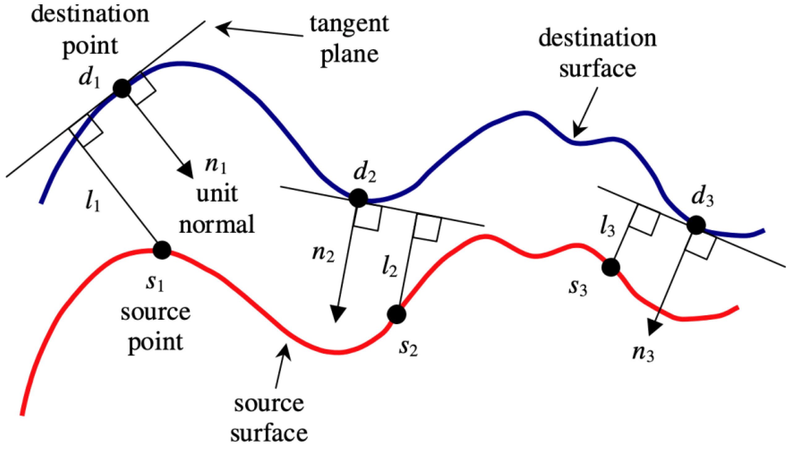
2.3. LiDAR Point Cloud Registration
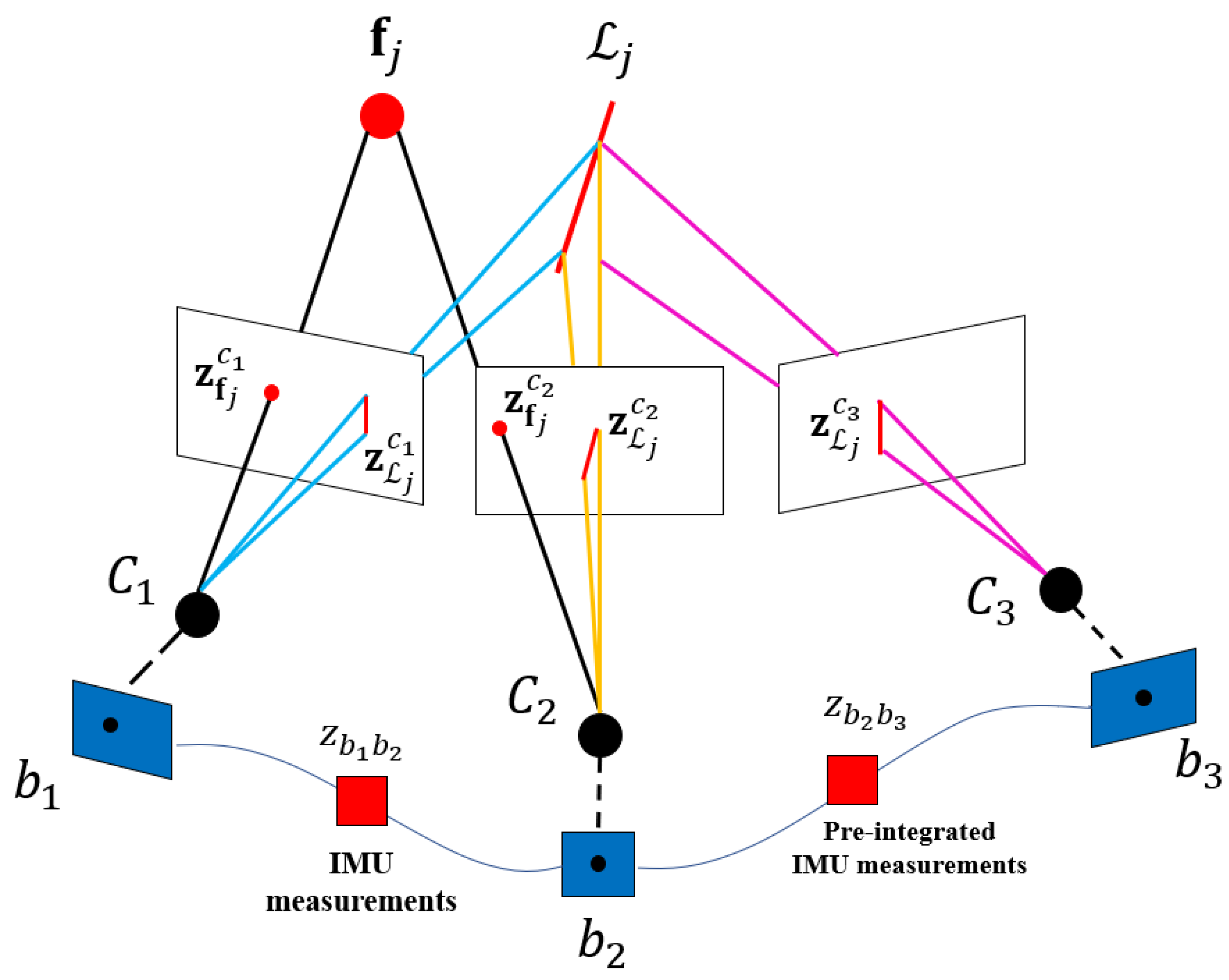
2.4. Tightly Coupled Nonlinear Optimization
- 2.
- IMU measurement residual: It is generated by IMU data between adjacent frames, including state propagation prediction and residuals of IMU pre-integration, namely in the optimization term. Optimization variables are IMU state ( and bias). The calculation of is shown as follows:
- 3.
- Visual residual: The visual reprojection error of the feature point in the sliding window is the error between the observed value and the estimated value of the same landmark point in the normalized camera coordinate system, namely in the optimization term. The calculation formula is as follows:
- 4.
- Jacobian residual matrix: The value of the feature point in frame projected to the camera coordinate system in frame is:
2.5. Relocation
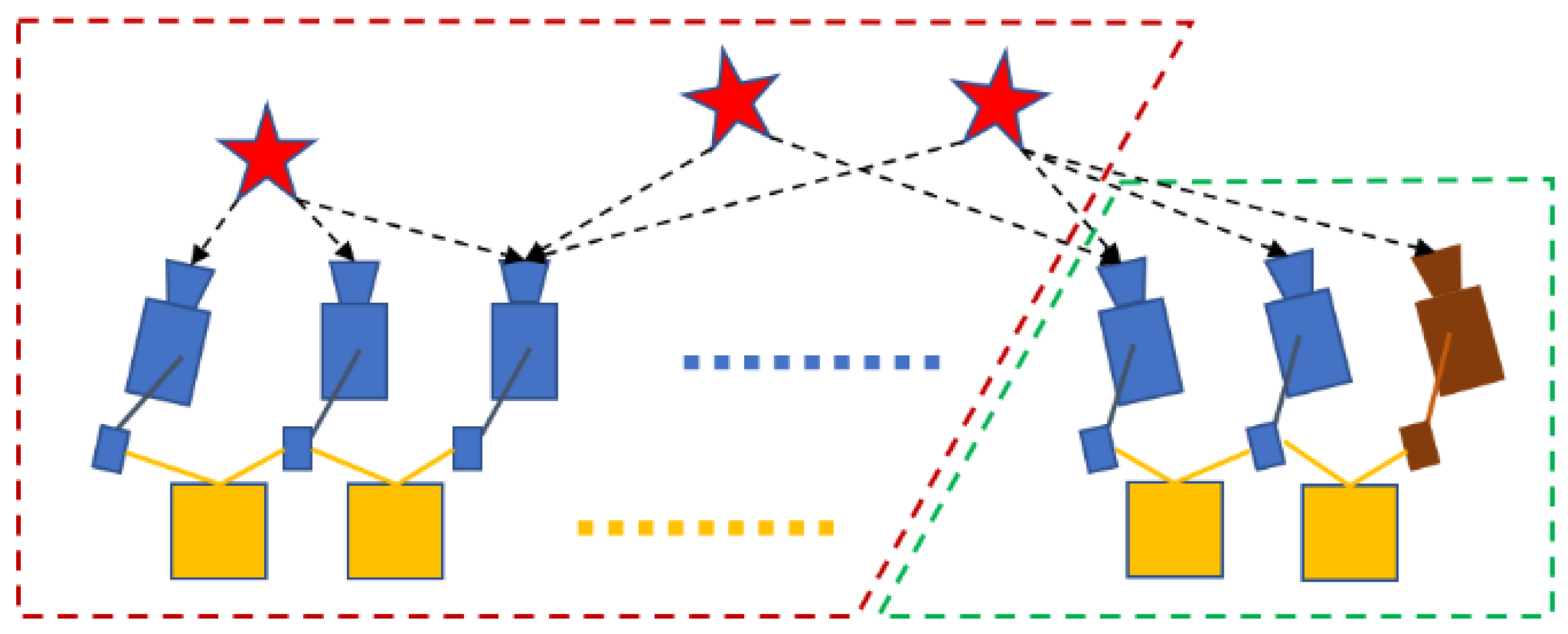
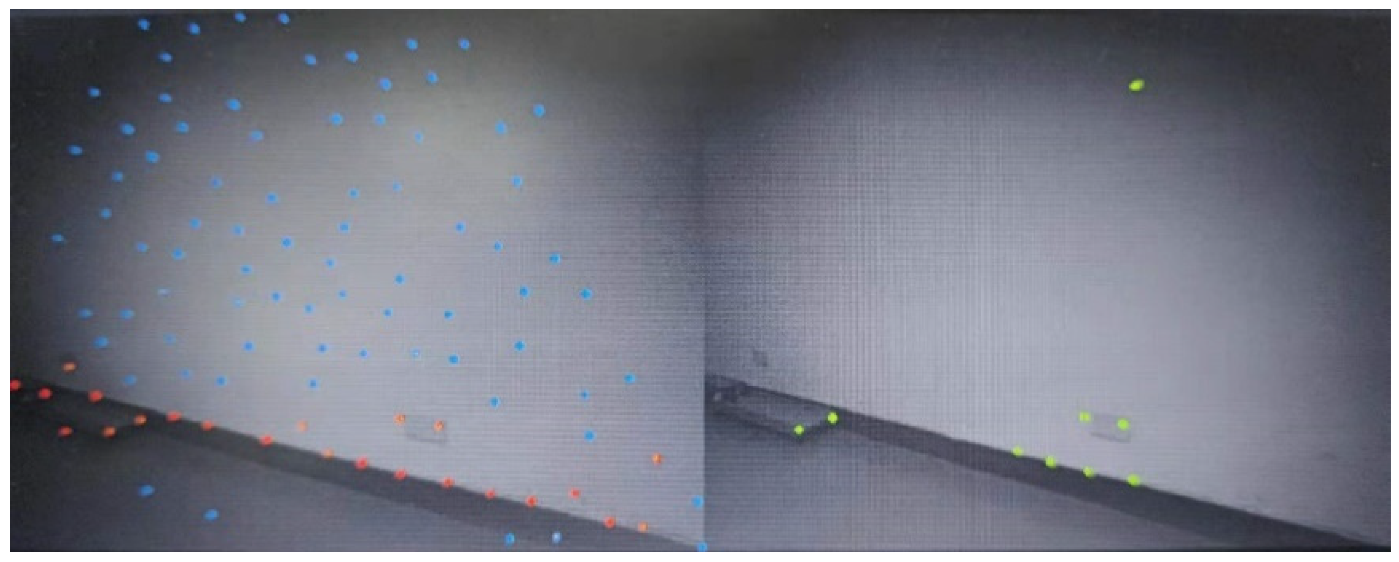
- First, visual word bag position recognition method (DBoW2) [38] is used for loop detection. During this period, only pose estimation is performed (blue part), and the past state (green part) is always recorded. After time and space consistency test, the visual word bag returns loopback detection candidate frames, and the red dotted line in the figure represents loopback association.
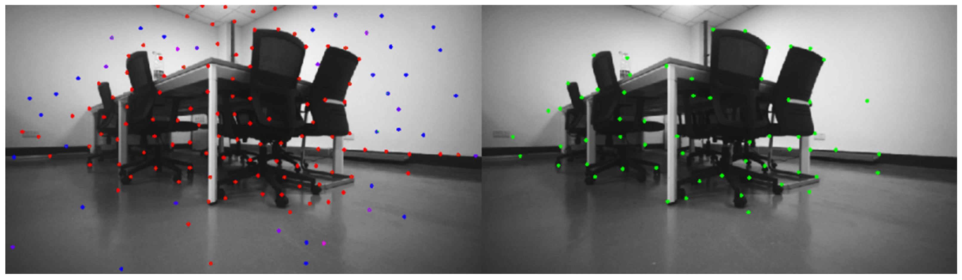
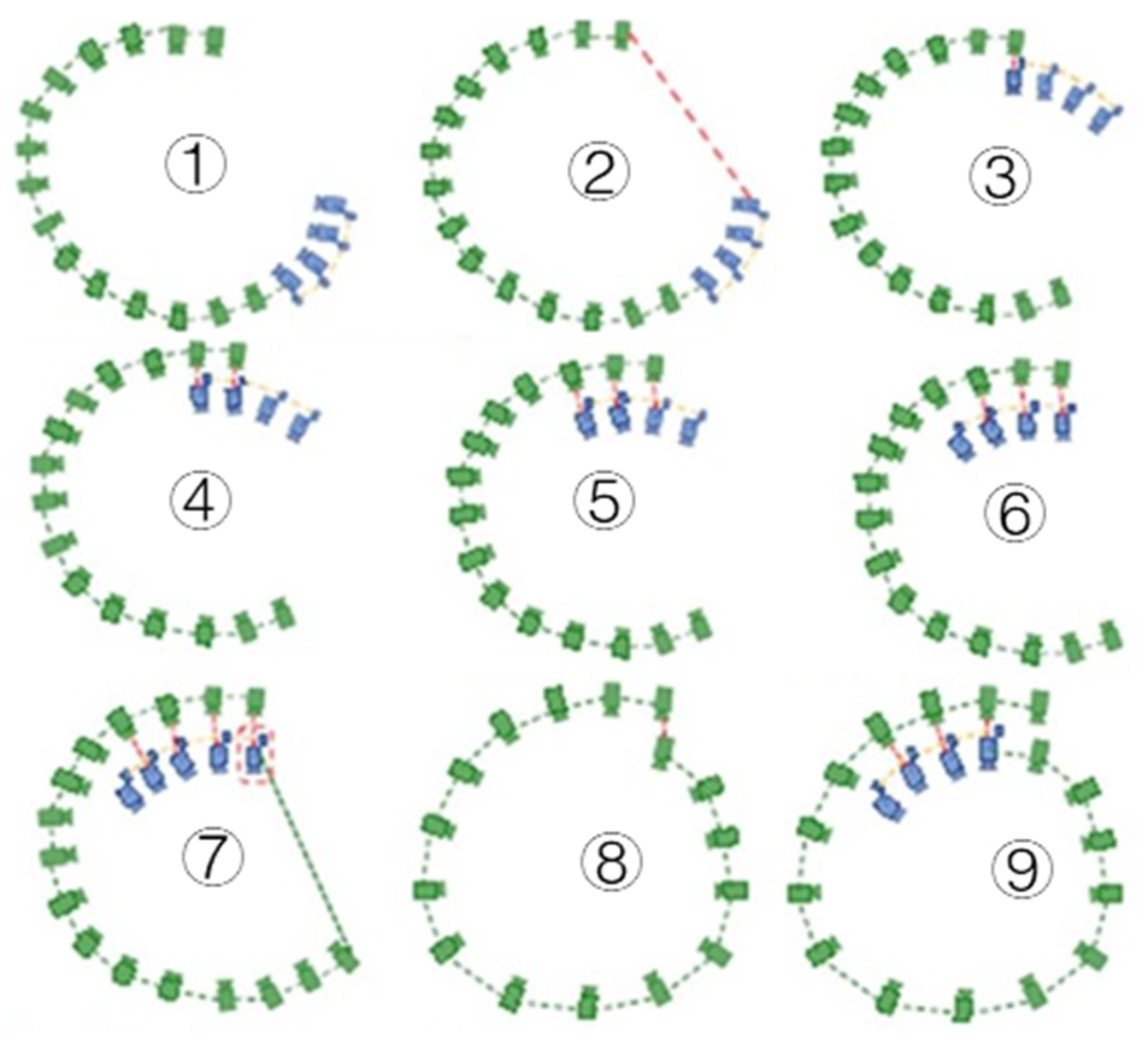
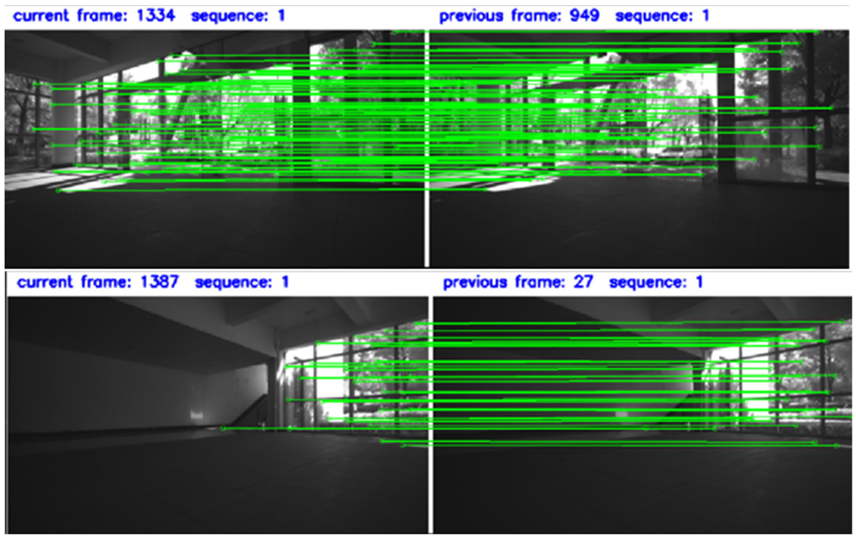
- If loopback is detected in the latest frame, the multi-constraint relocation is initiated, the corresponding relationship is matched by BRIEF descriptors [39], and the outer points are removed by two-step geometric elimination method (2D–2D, 3D–2D) [40]. When the inner point exceeds a certain threshold, the candidate frame is regarded as the correct loopback detection and relocation is performed. Feature matching of loopback candidate frames is shown in Figure 9.
- 3.
- Finally, key frames were added to the pose map, and the global 4-DOF (coordinate XYZ and yaw angle) pose optimization of the past pose and closed loop image frames are performed by minimizing the cost function:
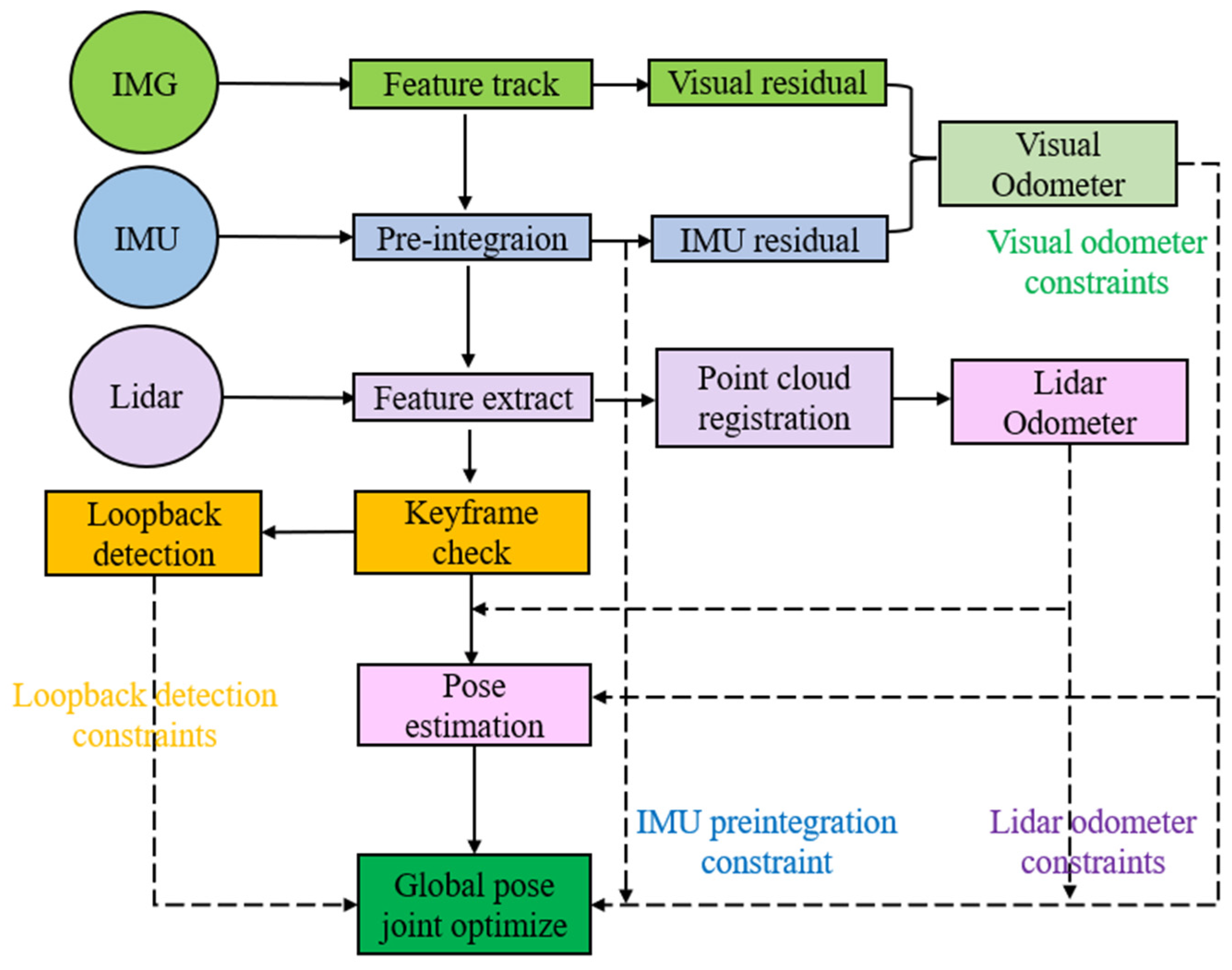
2.6. Algorithm Flow
- The input image data is used for feature point tracking by optical flow method, that is, the motion of the previous frame is used to estimate the initial position of feature points in the current frame. The positive and negative matching of both eyes was performed by LK optical flow method, and its error must be less than 0.5 pixel; otherwise, it is regarded as outlier. Then, the fundamental matrix (F) is calculated by using tracking points, and outliers are further removed using polar constraint [41]. If feature points are insufficient, corner points are used to replace them, and the tracking times of feature points are updated. Then the normalized camera coordinates of feature points and the moving speed relative to the previous frame are calculated. Finally, the feature point data of the current frame (including normalized camera plane coordinates, pixel coordinates, and normalized camera plane moving speed) are saved.
- After IMU data is input, IMU median integration is performed to calculate the current frame pose and update . The specific steps are using the IMU data between the previous frame and the current frame; if there is no initialization, the IMU acceleration between this frame is averaged, and the gravity is aligned to obtain the initial IMU attitude. Then the pose of the previous frame is applied it to IMU integral to obtain the pose of the current frame.
- The LiDAR odometer is obtained by extracting point cloud features and matching them with visual features. The feature graph is optimized in real time by sliding window.
- The estimation results of the laser odometer were used for initialization, and the depth information of the visual features was optimized using the LiDAR measurement results. The visual odometer was obtained by minimizing the visual residuals, IMU measurement residuals and marginalization residuals, and the pose estimation was performed.
- Key frame check: The criteria for confirming key frames is that there are many new feature points or the parallax of feature points in the first two frames is large enough [42]. After the keyframe check, the visual word bag method is used for loop detection.
- Global pose joint optimization: The whole state estimation task of the system is expressed as a maximum estimation posterior probability problem, and the global pose joint optimization is performed by IMU pre-integral constraint, visual odometer constraint, radar odometer constraint, and loopback detection constraint.
3. Results
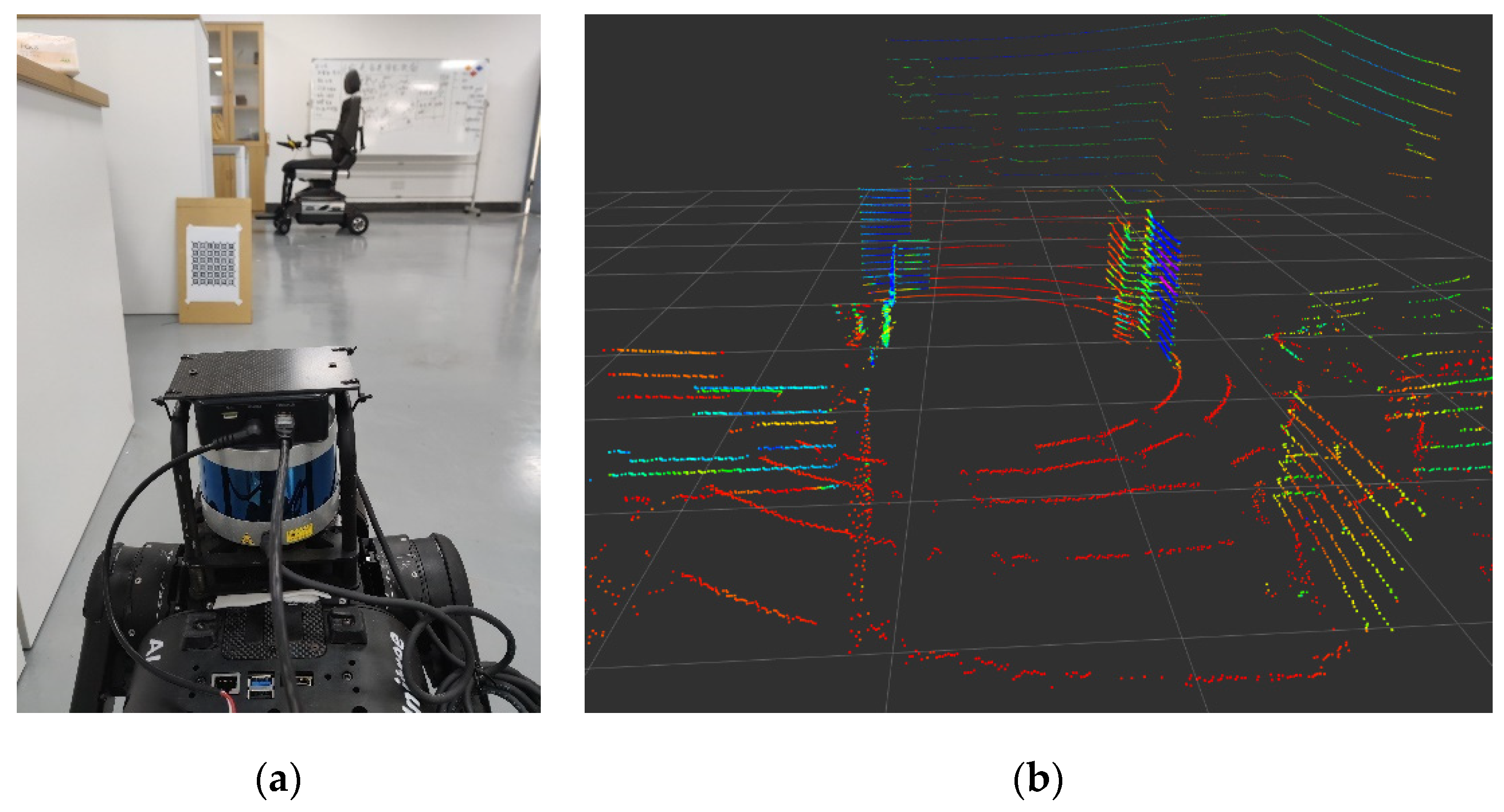
3.1. Experimental Platform and Environment
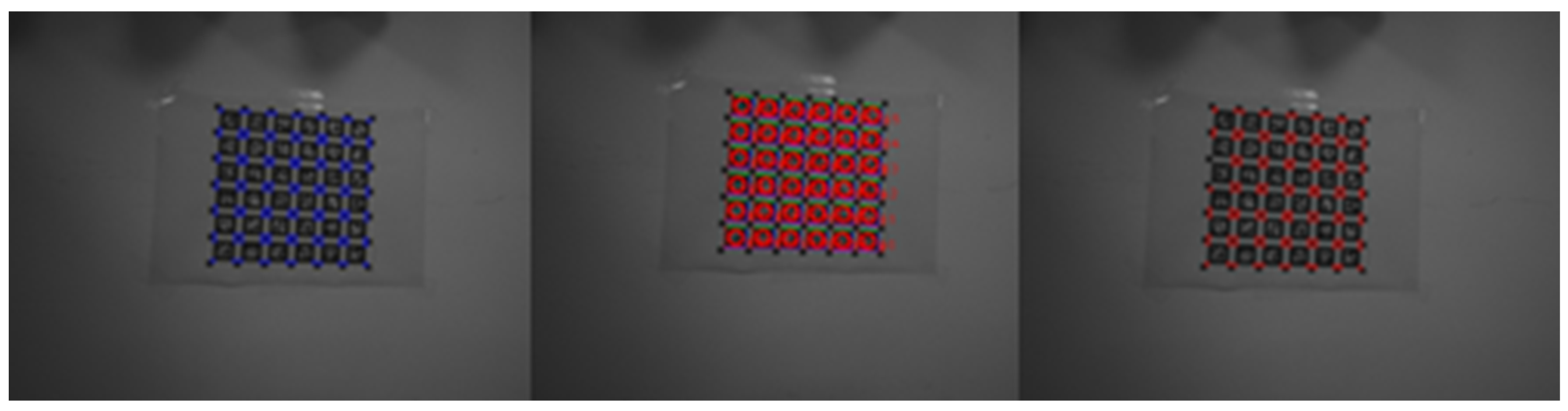
3.2. The Sensor Calibration
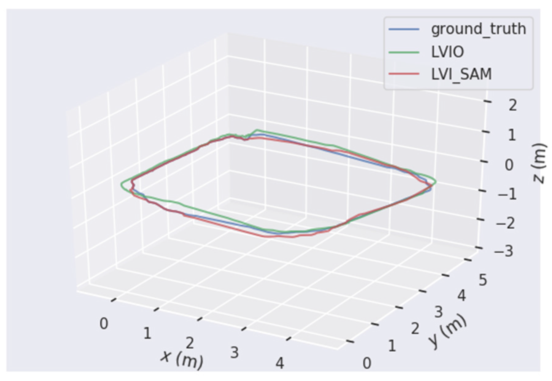
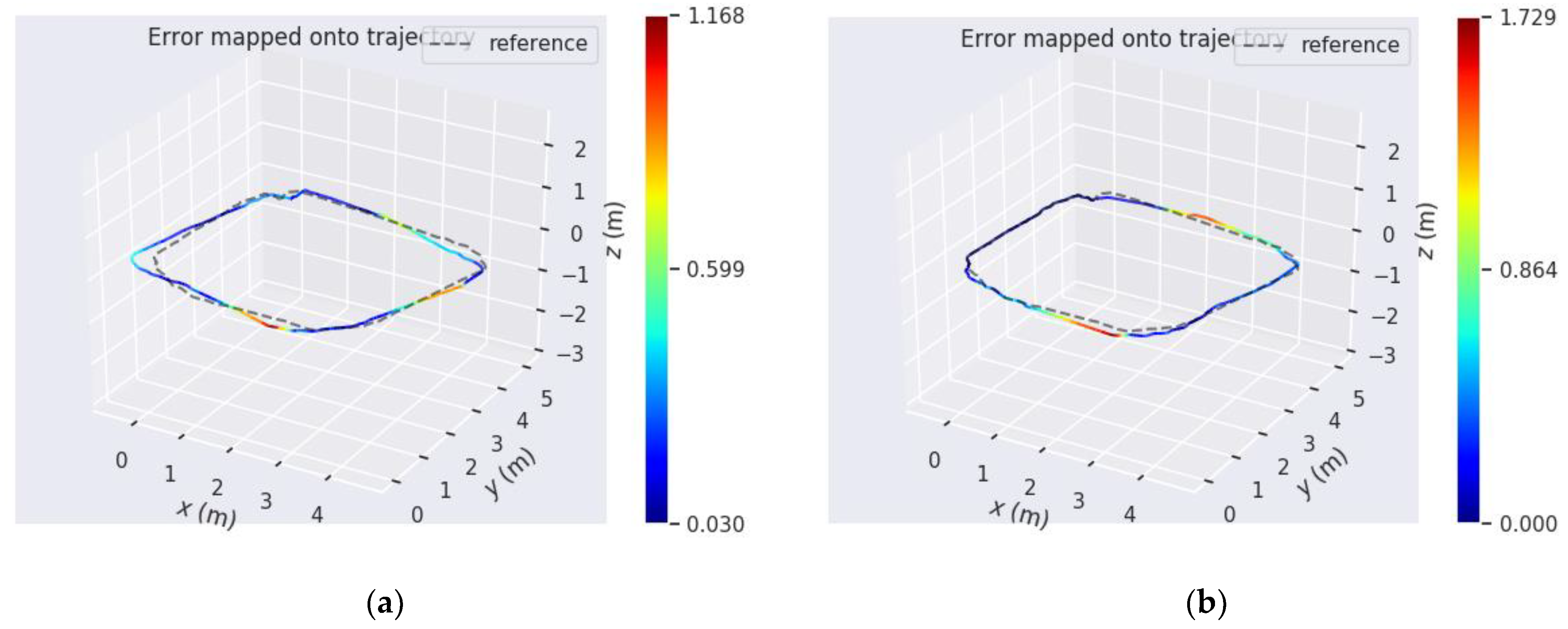
3.3. The Indoor Experiment
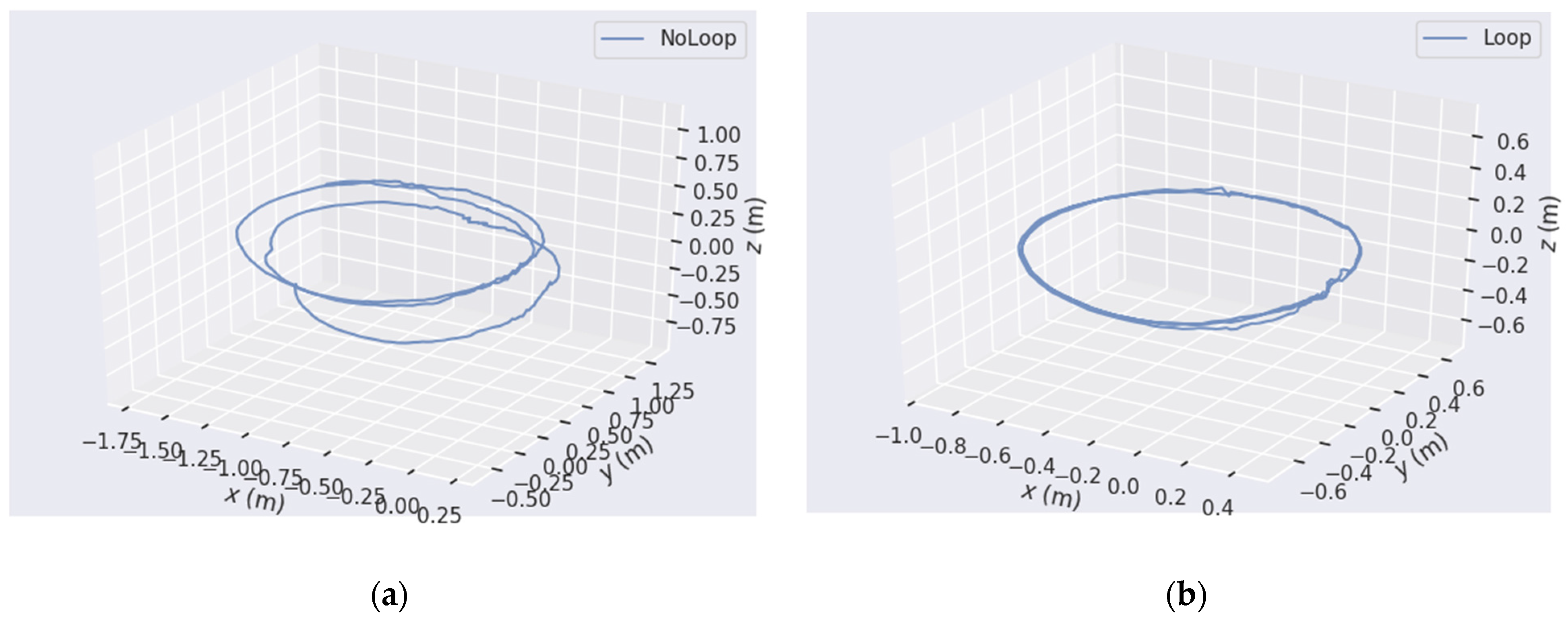
3.4. The Loop Detection Experiment
3.5. The Outdoor Experiments
4. Discussion
5. Conclusions
Author Contributions
Funding
Data Availability Statement
Conflicts of Interest
References
- Meng, X.; Wang, S.; Cao, Z.; Zhang, L. A review of quadruped robots and environment perception. In Proceedings of the Chinese Control Conference (CCC), Chengdu, China, 27–29 July 2016; pp. 6350–6356. [Google Scholar]
- Li, Z.; Ge, Q.; Ye, W.; Yuan, P. Dynamic balance optimization and control of quadruped robot systems with flexible joints. IEEE Trans. Syst. Man Cybern. Syst. 2015, 46, 1338–1351. [Google Scholar] [CrossRef]
- Prasad, S.K.; Rachna, J.; Khalaf, O.I.; Le, D.-N. Map matching algorithm: Real time location tracking for smart security application. Telecommun. Radio Eng. 2020, 79, 1189–1203. [Google Scholar] [CrossRef]
- Mowafy, A.; Kubo, N. Integrity monitoring for positioning of intelligent transport systems using integrated RTK-GNSS, IMU and vehicle odometer. IET Intell. Transp. Syst. 2018, 12, 901–908. [Google Scholar] [CrossRef] [Green Version]
- Li, F.; Tu, R.; Hong, J.; Zhang, H.; Zhang, P.; Lu, X. Combined Positioning Algorithm Based on BeiDou Navigation Satellite System and Raw 5G Observations. Measurement 2022, 190, 110763. [Google Scholar] [CrossRef]
- Jagadeesh, G.R.; Srikanthan, T. Online map-matching of noisy and sparse location data with hidden Markov and route choice models. IEEE Trans. Intell. Transp. Syst. 2017, 18, 2423–2434. [Google Scholar] [CrossRef]
- Nikolaev, D.; Chetiy, V.; Dudkin, V.; Davydov, V. Determining the location of an object during environmental monitoring in conditions of limited possibilities for the use of satellite positioning. In IOP Conference Series Earth and Environ-Mental Science; IOP Publishing: Bristol, UK, 2020; Volume 578, p. 012052. [Google Scholar]
- Subedi, S.; Kwon, G.R.; Shin, S.; Hwang, S.; Pyun, J. Beacon based indoor positioning system using weighted centroid localization approach. In Proceedings of the IEEE Eighth International Conference on Ubiquitous and Future Networks (ICUFN), Vienna, Austria, 5–8 July 2016; pp. 1016–1019. [Google Scholar]
- Nemec, D.; Šimák, V.; Janota, A.; Hruboš, M.; Bubeníková, E. Precise localization of the mobile wheeled robot using sensor fusion of odometry, visual artificial landmarks and inertial sensors. Robot. Auton. Syst. 2019, 112, 168–177. [Google Scholar] [CrossRef]
- Zhang, J.; Singh, S. Visual-lidar odometry and mapping: Low-drift, robust, and fast. In Proceedings of the IEEE International Conference on Robotics and Automation (ICRA), Seattle, WA, USA, 25–30 May 2015; pp. 2174–2181. [Google Scholar]
- Gui, J.; Gu, D.; Wang, S.; Hu, H. A review of visual inertial odometry from filtering and optimisation perspectives. Adv. Robot. 2015, 29, 1289–1301. [Google Scholar] [CrossRef]
- Taketomi, T.; Uchiyama, H.; Ikeda, S. Visual SLAM algorithms: A survey from 2010 to 2016. IPSJ Trans. Comput. Vis. Appl. 2017, 9, 1–11. [Google Scholar] [CrossRef]
- Sun, K.; Mohta, K.; Pfrommer, B.; Watterson, M.; Liu, S.; Mulgaonkar, Y.; Taylor, C.J.; Kumar, V. Robust stereo visual inertial odometry for fast autonomous flight. IEEE Robot. Autom. Lett. 2018, 3, 965–972. [Google Scholar] [CrossRef] [Green Version]
- Campos, C.; Elvira, R.; Rodríguez, J.J.G.; Montiel, J.M.M.; Tardós, J.D. Orb-slam3: An accurate open-source library for visual, visual–inertial, and multimap slam. IEEE Trans. Robot. 2021, 37, 1874–1890. [Google Scholar] [CrossRef]
- Qin, T.; Li, P.; Shen, S. Vins-mono: A robust and versatile monocular visual-inertial state estimator. IEEE Trans. Robot. 2018, 34, 1004–1020. [Google Scholar] [CrossRef] [Green Version]
- Heo, S.; Park, C.G. Consistent EKF-based visual-inertial odometry on matrix Lie group. IEEE Sens. J. 2018, 18, 3780–3788. [Google Scholar] [CrossRef]
- Ma, S.; Bai, X.; Wang, Y.; Fang, R. Robust stereo visual-inertial odometry using nonlinear optimization. Sensors 2019, 19, 3747. [Google Scholar] [CrossRef] [Green Version]
- Gargoum, S.; Basyouny, K. Automated extraction of road features using LiDAR data: A review of LiDAR applications in transportation. In Proceedings of the IEEE International Conference on Transportation Information and Safety (ICTIS), Banff, AB, Canada, 8–10 August 2017; pp. 563–574. [Google Scholar]
- Zhang, J.; Singh, S. LOAM: Lidar Odometry and Mapping in Real-time. Robot. Sci. Syst. 2014, 2, 1–9. [Google Scholar]
- Shan, T.; Englot, B.; Meyers, D.; Wang, W.; Ratti, C.; Rus, D. Lio-sam: Tightly-coupled lidar inertial odometry via smoothing and mapping. In Proceedings of the IEEE/RSJ International Conference on Intelligent Robots and Systems (IROS), Las Vegas, NV, USA, 24 October 2020; pp. 5135–5142. [Google Scholar]
- Shi, X.; Liu, T.; Han, X. Improved Iterative Closest Point (ICP) 3D point cloud registration algorithm based on point cloud filtering and adaptive fireworks for coarse registration. Int. J. Remote Sens. 2020, 41, 3197–3220. [Google Scholar] [CrossRef]
- Li, L.; Yang, F.; Zhu, H.; Li, D.; Li, Y.; Tang, L. An improved RANSAC for 3D point cloud plane segmentation based on normal distribution transformation cells. Remote Sens. 2017, 9, 433. [Google Scholar] [CrossRef] [Green Version]
- Pomerleau, F.; Colas, F.; Siegwart, R.; Magnenat, S. Comparing ICP variants on real-world data sets. Auton. Robot. 2013, 34, 133–148. [Google Scholar] [CrossRef]
- Lee, S.; Kim, C.; Cho, S.; Myoungho, S.; Jo, K. Robust 3-Dimension Point Cloud Mapping in Dynamic Environment Using Point-Wise Static Probability-Based NDT Scan-Matching. IEEE Access 2020, 8, 175563–175575. [Google Scholar] [CrossRef]
- Hutter, M.; Gehring, C.; Jud, D.; Lauber, A.; Bellicoso, C.D.; Tsounis, V.; Hwangbo, J.; Bodie, K.; Fankhauser, P.; Bloesch, M. Anymal-a highly mobile and dynamic quadrupedal robot. In Proceedings of the IEEE/RSJ International Conference on Intelligent Robots and Systems (IROS), Daejeon, Korea, 9–14 October 2016; pp. 38–44. [Google Scholar]
- Forster, C.; Carlone, L.; Dellaert, F.; Scaramuzza, D. On-manifold pre-integration for real-time visual-inertial odometry. IEEE Trans. Robot. 2016, 33, 1–21. [Google Scholar] [CrossRef] [Green Version]
- Plyer, A.; Le, B.G.; Champagnat, F. Massively parallel Lucas Kanade optical flow for real-time video processing applications. J. Real-Time Image Process. 2016, 11, 713–730. [Google Scholar] [CrossRef]
- Deray, J.; Solà, J.; Andrade, C.J. Joint on-manifold self-calibration of odometry model and sensor extrinsics using pre-integration. In Proceedings of the IEEE European Conference on Mobile Robots (ECMR), Prague, Czech Republic, 4–6 September 2019; pp. 1–6. [Google Scholar]
- Chang, L.; Niu, X.; Liu, T. GNSS/IMU/ODO/LiDAR-SLAM integrated navigation system using IMU/ODO pre-integration. Sensors 2020, 20, 4702. [Google Scholar] [CrossRef] [PubMed]
- Yuan, Z.; Zhu, D.; Chi, C.; Tang, J.; Liao, C.; Yang, X. Visual-inertial state estimation with pre-integration correction for robust mobile augmented reality. In Proceedings of the 27th ACM International Conference on Multimedia, Nice, France, 21–25 October 2019; pp. 1410–1418. [Google Scholar]
- Le, G.C.; Vidal, C.T.; H, S. 3d lidar-imu calibration based on upsampled preintegrated measurements for motion distortion correction. In Proceedings of the IEEE International Conference on Robotics and Automation (ICRA), Brisbane, Australia, 21–26 May 2018; pp. 2149–2155. [Google Scholar]
- Li, P.; Wang, R.; Wang, Y.; Tao, W. Evaluation of the ICP algorithm in 3D point cloud registration. IEEE Access 2020, 8, 68030–68048. [Google Scholar] [CrossRef]
- Kim, H.; Song, S.; Myung, H. GP-ICP: Ground plane ICP for mobile robots. IEEE Access 2019, 7, 76599–76610. [Google Scholar] [CrossRef]
- Shen, Y.; Feng, C.; Yang, Y.; Tian, D. Mining point cloud local structures by kernel correlation and graph pooling. In Proceedings of the IEEE Conference on Computer vision and Pattern Recognition, Salt Lake City, UT, USA, 18–23 June 2018; pp. 4548–4557. [Google Scholar]
- Sirtkaya, S.; Seymen, B.; Alatan, A.A. Loosely coupled Kalman filtering for fusion of Visual Odometry and inertial navigation. In Proceedings of the 16th International Conference on Information Fusion, Istanbul, Turkey, 9–12 July 2013; pp. 219–226. [Google Scholar]
- Von, S.L.; Usenko, V.; Cremers, D. Direct sparse visual-inertial odometry using dynamic marginalization. In Proceedings of the IEEE International Conference on Robotics and Automation (ICRA), Brisbane, Australia, 21–25 May 2018; pp. 2510–2517. [Google Scholar]
- Yang, L.; Ma, H.; Wang, Y.; Xia, J.; Wang, C. A Tightly Coupled Li-DAR-Inertial SLAM for Perceptually Degraded Scenes. Sensors 2022, 22, 3063. [Google Scholar] [CrossRef] [PubMed]
- Zhang, Q.; Xu, G.; Li, N. Improved SLAM closed-loop detection algorithm based on DBoW2. J. Phys. Conf. Series. IOP Publ. 2019, 1345, 042094. [Google Scholar] [CrossRef]
- Tafti, A.P.; Baghaie, A.; Kirkpatrick, A.B.; Holz, J.D.; Owen, H.A.; D’Souza, R.M.; Yu, Z. A comparative study on the application of SIFT, SURF, BRIEF and ORB for 3D surface reconstruction of electron microscopy images. Comput. Methods Biomech. Bio-Med. Eng. Imaging Vis. 2018, 6, 17–30. [Google Scholar] [CrossRef]
- Ferraz, L.; Binefa, X.; Moreno, N.F. Very fast solution to the PnP problem with algebraic outlier rejection. In Proceedings of the IEEE Conference on Computer Vision and Pattern Recognition, Columbus, OH, USA, 23–28 June 2014; pp. 501–508. [Google Scholar]
- Guan, B.; Yu, Y.; Su, A.; Shang, Y.; Yu, Q. Self-calibration approach to stereo cameras with radial distortion based on epipolar constraint. Appl. Opt. 2019, 58, 8511–8521. [Google Scholar] [CrossRef]
- Leutenegger, S.; Lynen, S.; Bosse, M.; Siegwart, R. Keyframe-based visual–inertial odometry using nonlinear optimization. Int. J. Robot. Res. 2015, 34, 314–334. [Google Scholar] [CrossRef] [Green Version]
- Shan, T.; Englot, B.; Ratti, C.; Rus, D. Lvi-sam: Tightly-coupled lidar-visual-inertial odometry via smoothing and mapping. In Proceedings of the IEEE International Conference on Robotics and Automation (ICRA), Xi’an, China, 30 May–5 June 2021; pp. 5692–5698. [Google Scholar]


 represents the old key frame,
  represents the latest frame,
  represents IMU constraint,
  represents visual feature,
  represents fixed state, and
  represents estimated state.
represents the old key frame, represents the latest frame, represents IMU constraint, represents visual feature, represents fixed state, and represents estimated state.
represents estimated state.
represents the old key frame, represents the latest frame, represents IMU constraint, represents visual feature, represents fixed state, and represents estimated state.


| Algorithm | LVIO Algorithm | Comparison Algorithm |
|---|---|---|
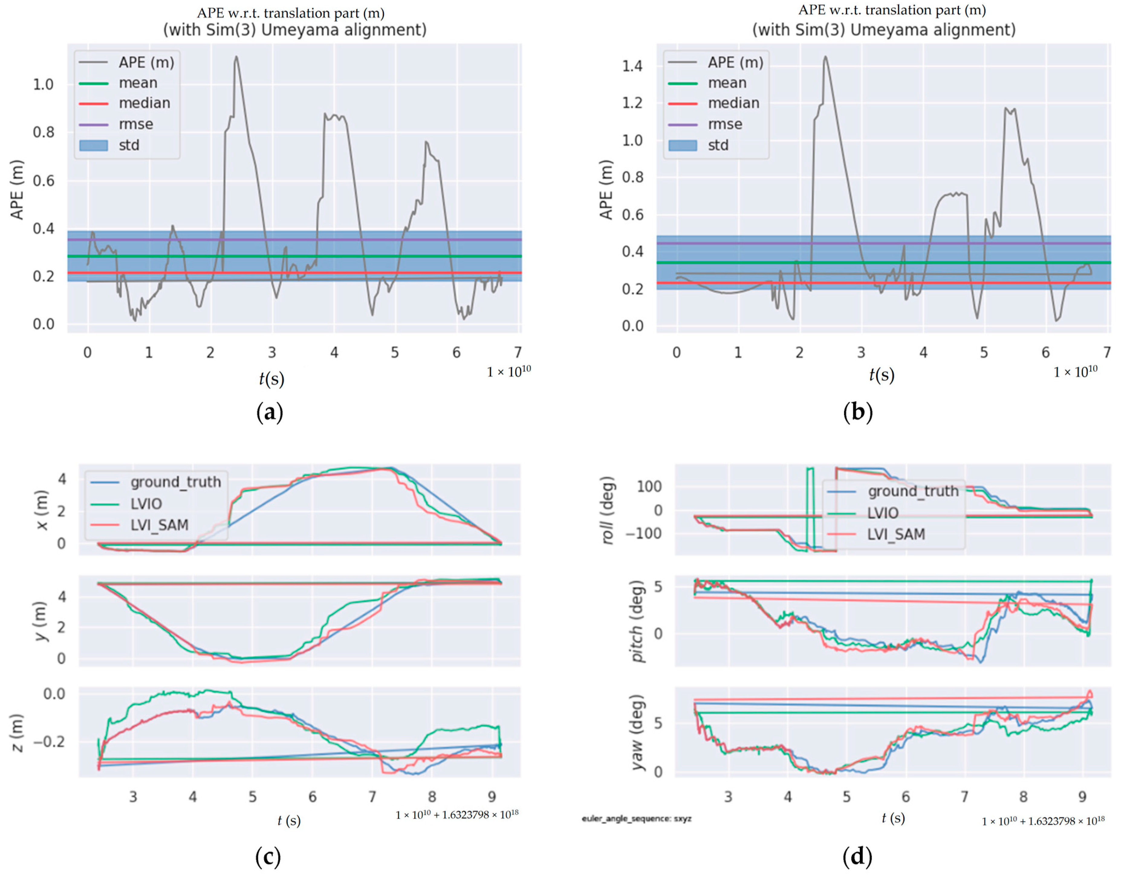
| Minimum error/m | 0.030335 | 0.000000 |
| Maximum error/m | 1.168070 | 1.728709 |
| Average error/m | 0.290409 | 0.306697 |
| Median error/m | 0.219200 | 0.131016 |
| Root mean square error/m | 0.358962 | 0.523203 |
| Standard error/m | 0.210989 | 0.423884 |
Publisher’s Note: MDPI stays neutral with regard to jurisdictional claims in published maps and institutional affiliations. |
© 2022 by the authors. Licensee MDPI, Basel, Switzerland. This article is an open access article distributed under the terms and conditions of the Creative Commons Attribution (CC BY) license (https://creativecommons.org/licenses/by/4.0/).
Share and Cite
Gao, F.; Tang, W.; Huang, J.; Chen, H. Positioning of Quadruped Robot Based on Tightly Coupled LiDAR Vision Inertial Odometer. Remote Sens. 2022, 14, 2945. https://doi.org/10.3390/rs14122945
Gao F, Tang W, Huang J, Chen H. Positioning of Quadruped Robot Based on Tightly Coupled LiDAR Vision Inertial Odometer. Remote Sensing. 2022; 14(12):2945. https://doi.org/10.3390/rs14122945
Chicago/Turabian StyleGao, Fangzheng, Wenjun Tang, Jiacai Huang, and Haiyang Chen. 2022. "Positioning of Quadruped Robot Based on Tightly Coupled LiDAR Vision Inertial Odometer" Remote Sensing 14, no. 12: 2945. https://doi.org/10.3390/rs14122945
APA StyleGao, F., Tang, W., Huang, J., & Chen, H. (2022). Positioning of Quadruped Robot Based on Tightly Coupled LiDAR Vision Inertial Odometer. Remote Sensing, 14(12), 2945. https://doi.org/10.3390/rs14122945