Technical Note

Improving WRF-Fire Wildfire Simulation Accuracy Using SAR and Time Series of Satellite-Based Vegetation Indices

1
Department of Geography and Environment, Bar-Ilan University, Ramat-Gan 5290002, Israel
2
Abiotix Environmental Services, Sderot Rothschild 17, Hadera 3820524, Israel
*
Author to whom correspondence should be addressed.
Remote Sens. 2022, 14(12), 2941; https://doi.org/10.3390/rs14122941
Submission received: 30 May 2022 / Revised: 14 June 2022 / Accepted: 16 June 2022 / Published: 20 June 2022

Abstract

:
Wildfire simulations depend on fuel representation. Present fuel models are mainly based on the density and properties of different vegetation types. This study aims to improve the accuracy of WRF-Fire wildfire simulations, by using synthetic-aperture radar (SAR) data to estimate the fuel load and the trend of vegetation index to estimate the dryness of woody vegetation. We updated the chaparral and timber standard woody fuel classes in the WRF-Fire fuel settings. We used the ESA global above-ground biomass (AGB) based on SAR data to estimate the fuel load, and the Landsat normalized difference vegetation index (NDVI) trends of woody vegetation to estimate the fuel moisture content. These fuel sub-parameters represent the dynamic changes and spatial variability of woody fuel. We simulated two wildfires in Israel while using three different fuel models: the original 13 Anderson Fire Behavior fuel model, and two modified fuel models introducing AGB alone, and AGB and dryness. The updated fuel model (the basic fuel model plus the AGB and dryness) improved the simulation results significantly, i.e., the Jaccard similarity coefficient increased by 283% on average. Our results demonstrate the potential of combining satellite SAR data and Landsat NDVI trends to improve WRF-Fire wildfire simulations.

Graphical Abstract

1. Introduction

Wildfires can cause direct damage to property and human lives, indirect damage to human health by wildfire smoke [1], damage to the environment by altering the functioning and structure of the ecosystem [2,3,4], and they can serve as a major source of greenhouse gas emissions that contribute to global warming [5]. In the Euro-Mediterranean region alone, a yearly average of c. 450,000 ha are burned [6], with the majority of fires being caused by anthropogenic activities [2,3]. Climate change and land-use/land-cover changes are projected to increase the frequency of wildfires in the Mediterranean region [7,8,9,10]. Wildland fires are highly complex phenomena determined by fuels, topography, and weather [11], but they are also greatly impacted by previous fires (e.g., fire interval and fire severity) and human activities [7]. They can be modeled as part of a large scale climate–vegetation–fire model such as FATES-SPITFIRE [12], as a single wildfire by using a two-dimensional semi-empirical model such as FARSITE [13], or by a much more computationally expensive model such as WRF-Fire [14], which is a numerical weather prediction (NWP) model combined with a 2D fire spread model that represents two-way fire–atmosphere interactions.
The results of these models depend on model inputs (fuel, topography, and weather), where fuel (distribution and quantity) is the only parameter that can be managed. Fuel mapping is therefore critical for improving the prediction of wildfire likelihood and intensity and for modeling fire behavior [15]. In many cases, it is the most important variable affecting the accuracy of the prediction of wildfire growth [16].
Fuel types refer to an identifiable association of fuel elements of different vegetation species, form, size, and height, as well as fuel density with a similar predicted fire behavior [17]. For example, the fuel loading is defined as the dry weight of the above-ground biomass (AGB) per unit area. Categorizing measurements into fuel classes usually results in a loss of fuel spatial heterogeneity [18]. Euro-Mediterranean standard fuel models tend to overestimate burned areas in contrast with local models that are based on field samples that better represent the local fuel [19].
LANDFIRE is the USA’s “standard” fuel maps product (provided for the continental USA). LANDFIRE maps are based on optical satellite and ground data and are used for modeling fire spatial behavior and spread in support of fire management decisions [20,21,22] as, for example, in operational wildfire simulations in Colorado [23]. CORINE is a land-cover maps product [24] provided through the EU’s “Copernicus” data hub. The operational fire modeling system in Greece uses CORINE as the basis for fuel model classification with the addition of custom fuel types based on the literature [25]. Operational wildfire simulations in Israel are based on government vegetation data maps that were converted into 13 fuel categories [26]. All of these fuel maps are based on the Scott and Burgan [27] and the Anderson [28] fuel model classification schemes.
Li et al. [29] used the time series of the MODIS and Landsat products and a standard fuel model to improve wildfire simulations. They used the MODIS NDVI and NPP products to estimate the annual accumulated AGB dead fuel load of shrubland/grassland fuel type in the Western USA. This information was used to update the fuel load in LANDFIRE, which improved the simulation of wildfire behavior with respect to the original LANDFIRE product. A similar approach, based on the Landsat vegetation structure index [30] and fuel accumulation model, was used to simulate wildfires in dry sclerophyll forests and woodlands in Western Australia [30].
It has been shown that in a Mediterranean climate, it is possible to map the AGB of woody vegetation by decomposing the NDVI time series into woody and herbaceous vegetation components [31,32]. The declining multi-year woody trend is used as a marker for increasing dry matter and the risk of wildfire spread [33,34] especially in dense Mediterranean woodlands [31,35]. Spaceborne synthetic-aperture radar (SAR) can supply direct information on fuel load (AGB) on the global scale (e.g., Sentinel-1 C band and L band PAL-SAR-2/ALOS-2 SAR). The SAR backscatter typically increases with the amount of AGB to the point of saturation [36]. This was used to assess Mediterranean forest biomass in central Italy [37] but is not commonly used [18]. Airborne SAR was also used to estimate the distribution of fuel load (AGB) for wildfire modeling in Yellowstone National Park [38].
The goal of this study was to improve the spatial representation of woody fuel, which is used as input in wildfire spread models in Mediterranean woodlands but which is missing in current fuel models [18]. We used the global SAR AGB product [39] to include the spatial representation of AGB, and the time series of NDVI woody vegetation [35] from Landsat to depict drying trends in woody vegetation that are related to the amount of dry matter [31,35]. Drying trends are not represented in current fuel models. The drying of woody vegetation is expected to intensify wildfire spread in the future [40] if the climate is drier. The effect of these changes in the representation of fuel on the predicted wildfire spread (area) will be examined here.
This methodology can be implemented, for example, by the Greek Fire Service forecasting system, which currently uses the open-source pan-European vegetation and land use datasets [25]. It can also be implemented in the operational wildfire system currently used in Israel [26].

2. Materials and Methods

The main focus of this study is to create a dynamic fuel model for input into the wildfire spread model. Figure 1 presents a flowchart summarizing the steps of this study. The dynamic fuel model is created by adding two components to the basic static fuel model: (a) the SAR-based fuel load (AGB), and (b) fuel moisture due to long-term dry periods as assessed by the trends of NDVI. These fuel models (static and dynamic), together with topography, and weather data are used to evaluate the potential improvement of the fire spread model.

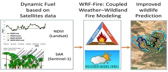
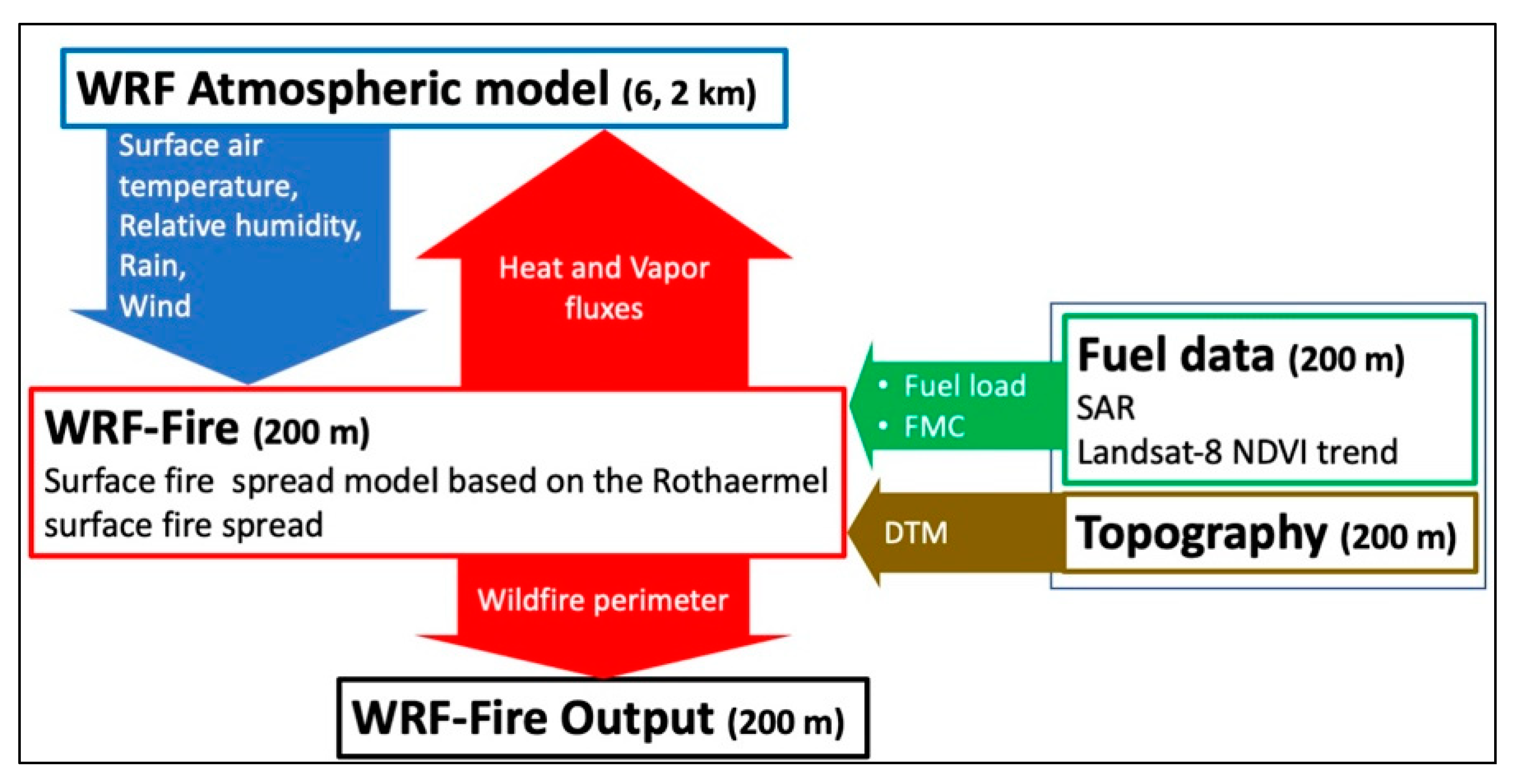
2.1. The Wildfire Prediction Model

For this study, we used the WRF-Fire wildfire modeling system, which is the operational system currently used in Israel [26]. WRF-Fire consists of the atmospheric model and the fire spread module based on Rothermel [41]. The WRF atmospheric model is a mesoscale numerical weather prediction model used for atmospheric research and operational forecasting applications. The model features a dynamical core that solves the fully compressible non-hydrostatic equations using terrain-following hydrostatic-pressure vertical coordinates and the Arakawa C-grid staggering spatial discretization for variables [42]. The atmospheric model was run on two one-way nested domains with horizontal grid spacings of 6000 m (D01) and 2000 m (D02), respectively. The fire spread module provides the two-way fire–atmosphere interactions modeling capability, which is schematically represented in Figure 2. Surface air temperature, relative humidity, rain, and wind were introduced from the WRF atmospheric model. Other inputs are the static topography layer, and the dynamic fuel load and moisture content which were changed in this study to assess their contribution to the predicted (output) wildfire perimeter. The fire module provides feedback to the atmospheric model through the surface heat and moisture fluxes.

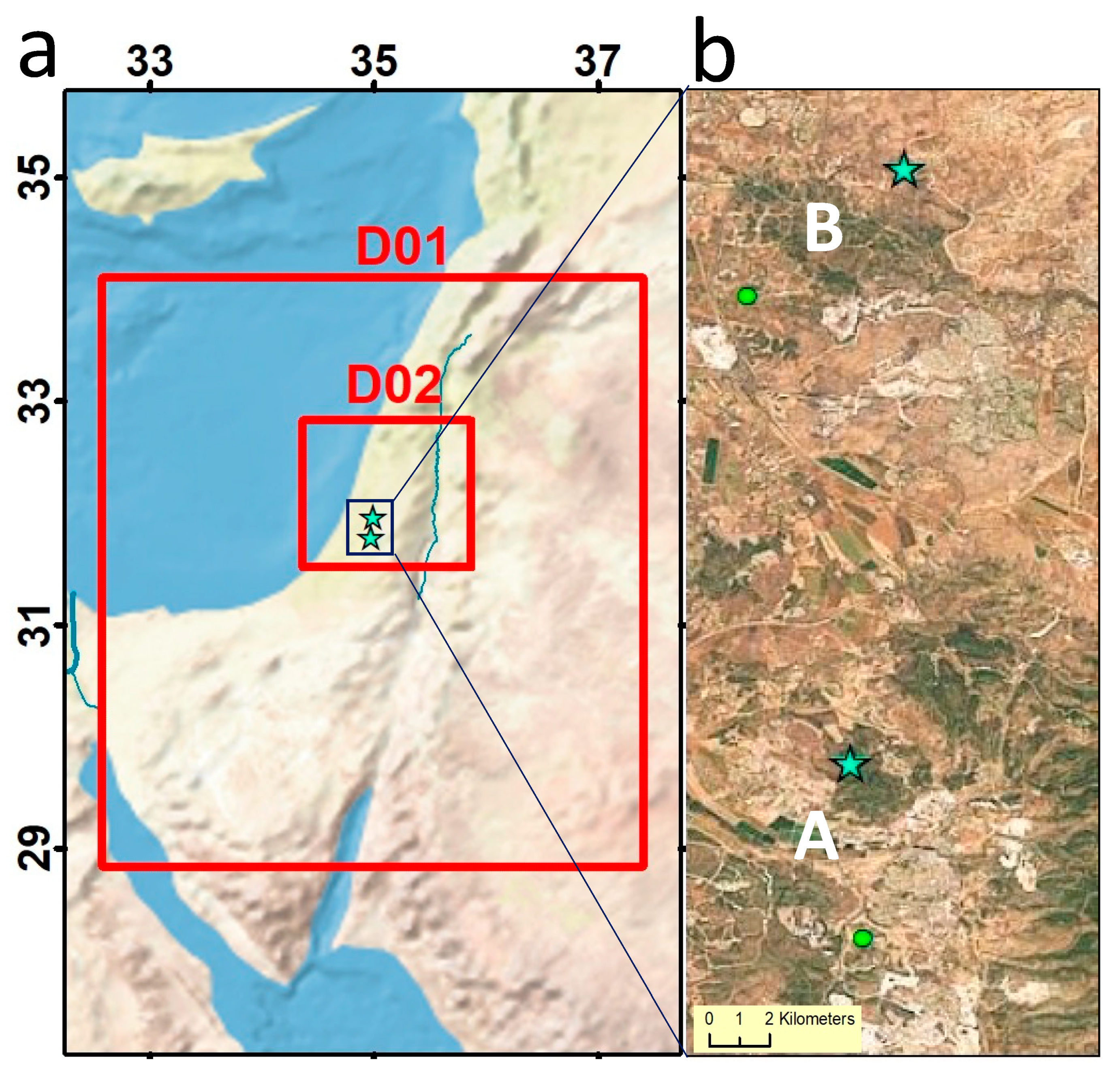
2.2. The Study Region

The region considered in this study is the center of Israel (Figure 3a,b). This region has a semi-arid, Mediterranean climate with a mean annual precipitation of 480 mm concentrated between December and March [43]. The woody vegetation in the area includes woodlands with intermixed trees and shrubs. There are shrublands with shrubs of 0.5–2 m height [44] and planted conifer forests mainly composed of native Pinus halfpennies pine and cypress species [45], which are usually more uniform in structure and composition [44]. Many of the wildfires occur in the late spring/early summer months (April–September) [46], while large fires are more common during spring and autumn under the influence of hot and dry synoptic systems. Large wildfires covering extensive areas have been associated with herbaceous vegetation, planted pine forests, and military training areas [33,47].
Two historical wildfires, which will be described below in Section 2.5, were used as case studies in this study. The locations of these two fires are indicated by the letters A and B in Figure 3b.

2.3. Fuel Maps

2.3.1. Base Fuel Map

We used the Israeli National Ecosystem Assessment Program 25 m spatial resolution 2016 vegetation formation map [48], which is based on several datasets including the Israeli operational wildfire forecasting system fuel map [26]. This fuel map was resampled to a spatial resolution of 100 m. A single static fuel model was assigned to each major vegetation formation based on the fuel classification [26] and was used as the base fuel map for the simulations (Table 1).

2.3.2. Base Fuel Map and AGB

The default settings for the AGB timber fuel model used a fixed value of 24.68 t ha−1 [28]. We used the 100 m spatial resolution global SAR AGB product for the year 2017, which is based on a combination of C Band (Sentinel-1) and L band (PAL-SAR-2/ALOS-2) SAR [39] to estimate three levels of timber (pine-dominated forest) AGB using natural breaks classification (low = 110; medium = 120; high = 130 t ha−1). Similarly, three levels of chaparral fuel type (original value of AGB 25.58 t ha−1) were set (low = 120, medium = 154, high = 180 t ha−1) (Figure 4c,g). The original AGB fuel values are based on the default fuel model which was developed in California [28].

2.3.3. Base Fuel Map, AGB, and Browning of Woody Vegetation (NDVI Woody Trend)

Landsat 8 NDVI data at 100 m spatial resolution (resampled from the original 30 m data) retrieved from Google Earth Engine [49] were decomposed into annual and woody vegetation [31,32]. The woody vegetation trend was calculated using five years (2013–2018) of the NDVI time series [35]. We used cloud-free yearly minimum NDVI which occurs in the mostly cloud-free dry summer. This approach takes advantage of the distinctive phenology of the main vegetation components (woody and herbaceous) in Mediterranean environments.
Decline in the 5-year woody vegetation trend is used as a marker for increasing dry matter which can be caused by drought [31,35,50]. Long-term effects of drought are not represented in the fuel model by a physical variable [28]. To overcome this limitation, we used the default amount of fuel moisture content (FMC) for each fuel class as a proxy for the woody vegetation trend. In areas with timber or chaparral fuel types with no significant negative trends (p > 0.1), we increased the FMC values by 25% based on several sensitivity tests (Figure 4c,g).

2.4. Configuration of the WRF-Fire Wildfire Modeling System
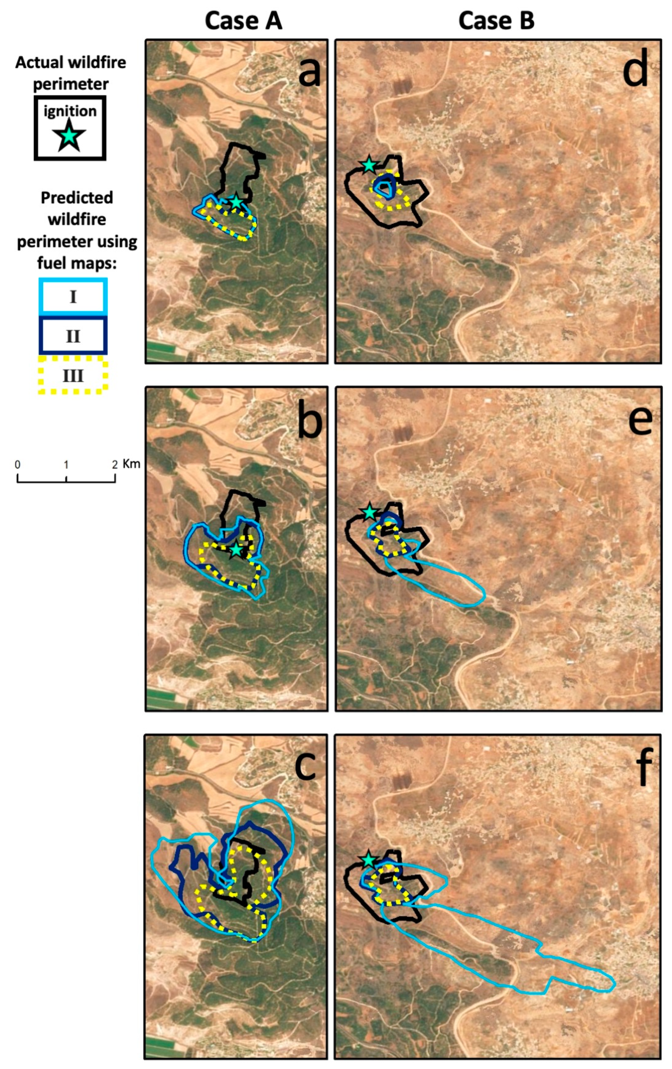
As noted above, the atmospheric component of WRF was configured to run on two one-way nested modelling domains with horizontal grid spacings of 6000 m (D01) and 2000 m (D02). Land use and soil type were represented using the default terrestrial datasets distributed by WRF [42]. The simulation of the wildfire spread was conducted at a high-spatial resolution, embedded as a sub-grid in D02 with a grid refinement ratio of 10:1 (Figure 3a), using the SRTM 90 m resolution global DEM.
Initial and lateral boundary conditions for WRF were extracted from publicly available forecast data from the National Centers for Environmental Prediction (NCEP) Global Forecasting System (GFS) with a spatial resolution of 0.25 degrees and a 3-h temporal resolution. The WRF simulations started at 00:00 (local time), while the fire began 8 h later. The updated fuel and FMC values were introduced by changing the WRF-Fire name list of fuel parameters and updating the spatial fuel input data of surface fuel [42].

2.5. Case Studies

The model was used to simulate two wildfire cases which have different characteristics in terms of the amount of woody vegetation. The locations are indicated above in Figure 3b. Following is a brief description of the two cases.
Case A. On 23 May 2019, a major wildfire broke out in the northern zone of the Tzora forest, which is a mature pine forest planted in the year 1950 by the Keren Kayemet Le’Israel–Jewish National Fund (KKL–JNF) and is situated north of the city of Beit Shemesh [43]. The fire ignition occurred in the morning during an extreme heatwave with a mean air temperature of 38.5 °C and a relative humidity of 10.3% between the hours of 8:00–17:00 as measured at the meteorological station of the Israel Meteorological Service (IMS), south of the Tzora forest (Figure 3b and Figure 4a–d). The spread of the fire towards the north was driven mainly by a gentle slope. It ended between noon and evening of the same day after burning 32.4 ha of adult pine [43]. This case was one of the many wildfires that occurred during the same week and was chosen to represent a fire in a dense conifer forest.
Case B. On 16 May 2019, a wildfire broke out in a low-elevation woodland area in the Northern Judean Mountains, northeast of the city of Modi’in-Maccabim-Re’ut (Figure 3b). The weather was normal for the season with a mean air temperature of 31.8 °C and a relative humidity of 48.5% as measured at the closest meteorological station of the Ministry of Agriculture (Figure 3b and Figure 4e–h). The fire started in the woodland area and spread towards the southeast driven by a mild slope and westerly winds. It was extinguished by nightfall. A total of 63.5 ha of mainly Pinus halepensis Mill and local shrub species were burned. This case was chosen to represent fire in a woodland area with a low density of woody vegetation.
In both cases, the ignition coordinates were estimated using MODIS and VIIRS hotspot data [51,52]. The ignition time was assumed to be 8:00 a.m. local time in both cases, and the actual wildfire perimeter was taken from the KKL–JNF database [7]. The perimeter represents all of the burned areas.
Each wildfire case was run with the original fuel map and with our two new fuel maps as listed in Table 2. We expect the fuel maps with additional details to positively affect the simulations. In general, we assume that the results of the simulations will be useful only for the first 3–4 h of the forecast [53], since the model does not consider external activities (e.g., firefighters’ or civilians’ actions) that may affect the spread of the fire. In Israel, most wildfires occur close to populated areas [7], and therefore firefighter response is usually rapidly activated in order to minimize the risk to life and property.

2.6. Comparing the Performance

We assessed the skill of the forecasts of the different fuel maps using the Jaccard similarity coefficient, in which the value is defined as the area of the intersection of the observed and simulated fire areas divided by the area of the union of the observed wildfire perimeter and the simulated wildfire [54]. The values range is between 0 and 1, where 1 means perfect similarity between the wildfire and the simulation, and 0 means no similarity [54,55]. The Jaccard similarity index is defined as:
J ( A , B ) = | A B | | A B | = | A B | | A | + | B | | A B | .
where A and B are the actual and simulated wildfire areas, respectively.

3. Results

3.1. Model Performance with Different Input Fuel Maps
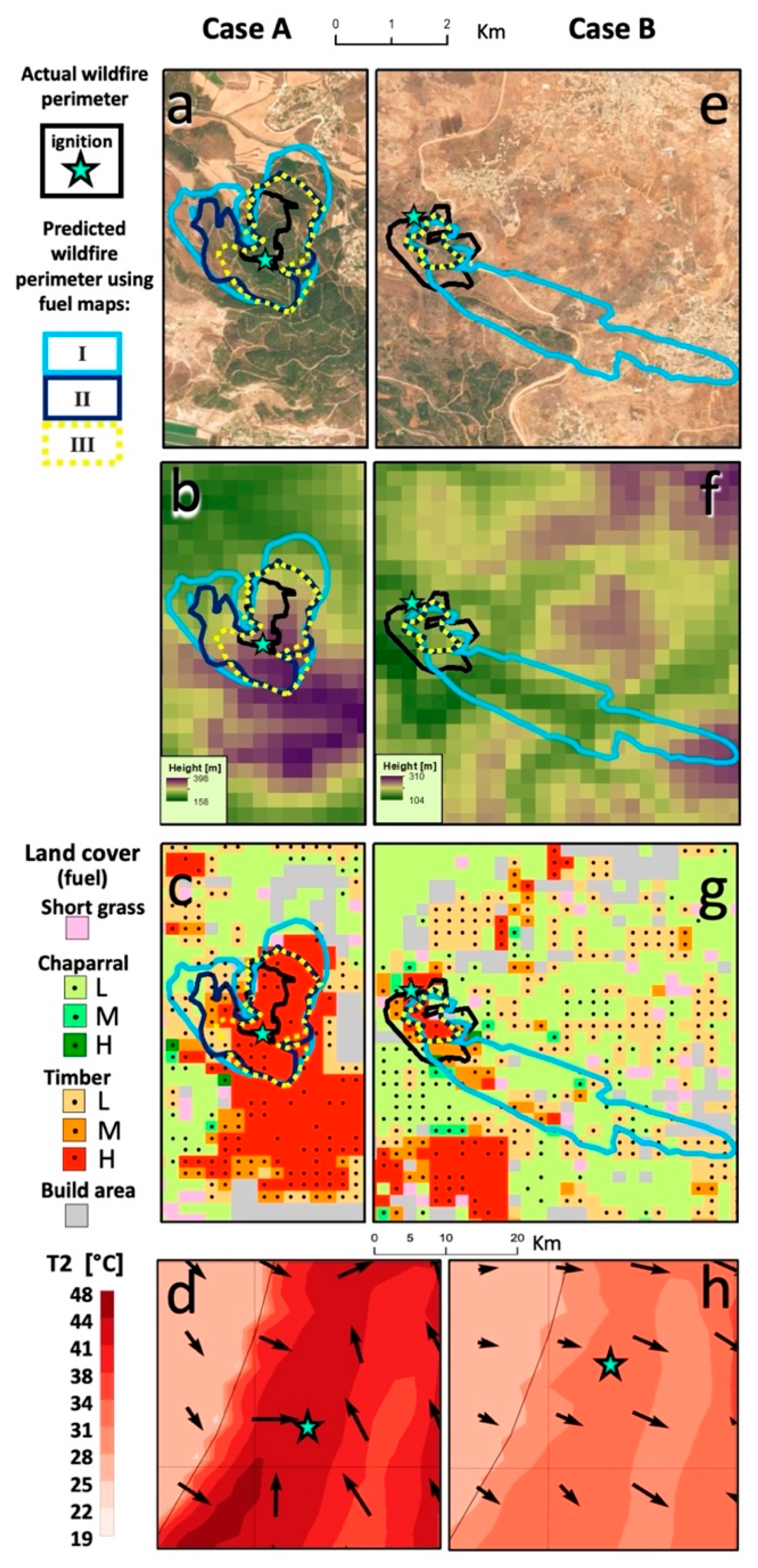
Table 3 summarizes the performance of the simulated wildfire perimeter using the model with the three different fuel maps, assessed using the Jaccard similarity coefficient. In both cases, A and B, the accuracy when using the basic fuel map is quite low with a value of 0.13. Similar results were obtained in a previous study [25]. The simulations in case A which were in a dense conifer forest show an improvement in performance between fuel model II and III, while in the case B woodland area, with a low density of woody vegetation, a similar performance is seen for fuel models II and III.

3.2. Case A

Figure 4a–c, show the results for the pine forest area of case A with the actual and predicted fire perimeters superimposed on the geographical map (Figure 4a), the topography map (Figure 4b), and the land-cover fuel map (Figure 4c) four hours after ignition. Meteorological conditions showing the 12 h WRF predicted 2 m temperature (extreme weather/heatwave) and the wind vectors are shown in Figure 4d for the 23 May 2019 event. The black line in each map shows the actual perimeter, while the results of the WRF-Fire simulations using the three fuel maps listed in Table 2 are indicated by the light blue, dark blue, and yellow lines for fuel maps I, II, and III, respectively. The observed perimeter indicates that the fire spread mainly to the north and northeast. All simulations show the advance of the wildfire to the north in a downslope direction, which is the same as the WRF-predicted wind direction. With fuel maps I and II, the model predicted the fire spreading to the south as well as to the northeast and northwest. The simulation skill (Jaccard similarity coefficient) of fuel map II was 292% higher than in the simulations with the original fuel map I. The simulation with fuel map III shows the best forecasting skill, which is 369% higher than the simulation with base fuel map I. It correctly restricts the wildfire from spreading too far out of the forest to the northwest, although it does show the spread to the south as in the other two simulations.

3.3. Case B

Figure 4e–g, show the results of case B in the WRF-Fire simulation 4 h after fire ignition, with the actual and predicted fire perimeters superimposed on the geographical map (Figure 4e), the topography map (Figure 4f), and the land-cover fuel map (Figure 4g) with the wildfire moving upslope in a southeast direction. Meteorological conditions for the 12 h WRF predicted 2 m temperature and wind vectors are shown in Figure 4g. The wildfire perimeter from the KKL–JNF data is shown in black. The simulation based on the original fuel map I progressed too far to the southeast, significantly overestimating the wildfire area in the downwind direction along the ridge and then downslope. The results of the simulations with fuel maps II and III were similar, with both significantly restricting the incorrect predicted spread to the southeast as seen in fuel map I. However, both underestimated the wildfire perimeter. The forecast skill of fuel maps II and III showed an improvement of 153% compared to the results from the simulation using base fuel map I.

4. Discussion

Adding more datasets and details (SAR, NDVI trends) to the fuel maps is expected to improve the model performance, although it may also potentially increase uncertainty. The new datasets were added in two stages in this study. Adding SAR-based AGB improved the Jaccard similarity coefficient in both cases (A and B). This improvement is attributed to the inclusion of spatial representation of the fuel load, which was lacking in the original fuel model. Adding NDVI trend-based information improved the Jaccard similarity coefficient in case A (forest) but not in case B (area with sparse woody vegetation). These results are in accordance with similar findings in Greece [35]. Following is a brief discussion of the effects of different aspects of the fuel maps on the model performance.

4.1. General Predictability of the WRF-Fire Model

As in [25], here too, the WRF-Fire simulation correctly captured the general direction of the wildfire spread. The fuel parameters affected only the rate of spread (ROS) while preserving the general shape of the fire perimeter. ROS values in the forest area were lower as was also reported in a study based on FARSITE wildfire simulations, probably due to down-slope wind flow, which slowed down the ROS in the forest area [56]. Furthermore, in Case A, significant shifts in the wind directions may have also helped limit the spread of the fire. The WRF-Fire prediction results produced relatively low skill probably due to the lack of calibration of the ROS, which has been shown to improve the skill of the model by up to 100% and, in some cases, even more [25].

4.2. Fuel and AGB

AGB values of the woody vegetation fuel type from the CCI biomass product [39] were similar to those reported in studies conducted in Mediterranean forests in Spain [57,58] and Northern Israel [32]. These values are much higher than the AGB values of the 13 fuel-type model that was developed for the Mediterranean climate of California [26,28] and that is used in the Israeli operational WRF-Fire forecasting system. The AGB values of timber and chaparral are fixed and lower than the spatially variable SAR product estimation (Figure 4c,g), which is one of the sources of errors in wildfire simulation [59,60].
The higher AGB values improved the characterization of the fuel, and therefore improved the skill of the model (Table 3) by reducing the overestimation of the perimeter errors (Figure 4a,e). A simulation of wildfires in other Mediterranean landscapes that included a standard pine tree fuel-type model and a customized fuel type with a higher AGB [19] also reported a reduction in the overestimation errors. Similar reductions in errors were reported in Mediterranean shrubland [56]. In the California king Megafire WRF-Fire simulation [61], reducing AGB values caused an amplification of the ROS. This effect was probably due to the self-reinforcing dynamics of fire-generated winds, rather than direct effects imposed by individual external factors such as fuel or drought [61].

4.3. Fuel, AGB, and NDVI Trend

Adding NDVI trend information improved the model performance in a high-AGB dense pine forest (case A), but not in the lower-AGB woodland (case B). The NDVI trend information was introduced to the model by adding 25% FMC to all areas, which did not show a significant negative NDVI trend (p > 0.1). The different effects of NDVI trends in low and high AGB woodlands were observed in another Mediterranean environment, in Greece, where the amount of fuel had a stronger effect on the wildfires than the amount of dead fuel [35]. Also, the effect of a negative NDVI trend (higher dead fuel) was significant only in a dense forest case as was shown in [35] where the relative influence of the amount of dead fuel was very low and increased with the amount of biomass.

4.4. Limitations of the Study

We acknowledge some limitations of this study. These include: (a) the estimation of the ignition point location using hotspot data based on MODIS and VIIRS as was done in [62,63]; (b) the assumption regarding the impact of rapid deployment of firefighting forces to wildfires in Israel is reasonable as almost all wildfires are close to populated areas, including the wildfires studied here in cases A and B; (c) errors are also introduced to the predicted fire due to the WRF-Fire representation of fire propagation as only a surface fire [60,64]; and (d), in this study, browning was modeled as a binary value. We recommend modeling the long-term effects (NDVI trends) in combination with the short-term effects (dynamic FMC, NDWI) in WRF-Fire [26], which was also suggested by [34].

5. Conclusions

In this study, we have demonstrated the advantage of running wildfire simulations using a high spatial resolution, global SAR AGB product, which provides the spatial variability of a given fuel type of woody vegetation. Using AGB from the global SAR product can reduce the need for expensive field measurements and appears to be able to improve regional wildfire spread forecasting systems such as the operational system in Greece that is currently based on the CORINE land-cover map for the fuel model [24], which is probably one of the sources of error in fire spread simulations [25].
In addition, we showed that incorporation of trends into the vegetation index of woody vegetation in Mediterranean climate regions may improve the results of wildfire simulation in dense forests through a better representation of the dryness status of woody vegetation due to the cumulative effects of drought. Nevertheless, further examination of the best method of integrating this information into the latest version of the WRF-Fire or other wildfire prediction systems is required. This may be especially relevant when considering new remote sensing data from global SAR which are expected to be available in the next few years.

Author Contributions

Y.M., G.K., S.B., I.M.L.—Conceptualization; Y.M., G.K.—Data preparation; Y.M.—Formal analysis; Y.M.—Funding acquisition; Y.M., G.K., S.B., I.M.L.—Investigation and Methodology; Y.M.—Project administration; Y.M., G.K., S.B., I.M.L.—Resources; Y.M., G.K.—Software; I.M.L., S.B.—Supervision; Y.M., G.K., S.B., I.M.L.—Validation; Y.M., I.M.L.—Visualization; Y.M.—Writing—original draft; Y.M., I.M.L., S.B.—Writing—review & editing. All authors have read and agreed to the published version of the manuscript.

Funding

This research was funded by the Israeli Ministry of Science, Technology and Space, Eshkol Scholarship (grant 3-14504).

Data Availability Statement

Landsat data can be obtained from Google Earth Engine (https://earthengine.google.com/). The vegetation formation map of Israel was obtained from Israeli National Ecosystem Assessment ([email protected]).

Acknowledgments

This work was conducted as part of Y.M.’s Ph.D. dissertation. Y.M. acknowledges the support provided by the Ministry of Science and Technology of Israel through the Eshkol Scholarship (grant 3-14504). The authors also thank the Jewish National Fund (KKL–JNF) for the wildfire perimeter database.

Conflicts of Interest

The authors declare no conflict of interest. The funders had no role in the design of the study; in the collection, analyses, or interpretation of data; in the writing of the manuscript, or in the decision to publish the results.

Appendix A

Figure A1. The WRF-Fire simulation results for the three fuel maps are shown for 9:00 (a,d), 10:00 (b,e), and 11:00 AM (c,f) local time.
Remotesensing 14 02941 g0a1

References

  1. Burke, M.; Driscoll, A.; Heft-Neal, S.; Xue, J.; Burney, J.; Wara, M. The changing risk and burden of wildfire in the United States. Proc. Natl. Acad. Sci. USA 2021, 118, e2011048118. [Google Scholar] [CrossRef] [PubMed]
  2. Borrelli, P.; Panagos, P.; Langhammer, J.; Apostol, B.; Schütt, B. Assessment of the cover changes and the soil loss potential in European forestland: First approach to derive indicators to capture the ecological impacts on soil-related forest ecosystems. Ecol. Indic. 2016, 60, 1208–1220. [Google Scholar] [CrossRef]
  3. Molina-Terrén, D.M.; Xanthopoulos, G.; Diakakis, M.; Ribeiro, L.; Caballero, D.; Delogu, G.M.; Viegas, D.X.; Silva, C.A.; Cardil, A. Analysis of forest fire fatalities in Southern Europe: Spain, Portugal, Greece and Sardinia (Italy). Int. J. Wildl. Fire 2019, 28, 85–98. [Google Scholar] [CrossRef] [Green Version]
  4. Pausas, J.G.; Llovet, J.; Rodrigo, A.; Vallejo, R. Are wildfires a disaster in the Mediterranean basin?—A review. Int. J. Wildl. Fire 2008, 17, 713. [Google Scholar] [CrossRef]
  5. Kim, B.; Sarkar, S. Impact of wildfires on some greenhouse gases over continental USA: A study based on satellite data. Remote Sens. Environ. 2017, 188, 118–126. [Google Scholar] [CrossRef]
  6. Polinova, M.; Wittenberg, L.; Kutiel, H.; Brook, A. Reconstructing pre-fire vegetation condition in the wildland urban interface (WUI) using artificial neural network. J. Environ. Manag. 2019, 238, 224–234. [Google Scholar] [CrossRef]
  7. Levin, N.; Tessler, N.; Smith, A.; McAlpine, C. The Human and Physical Determinants of Wildfires and Burnt Areas in Israel. Environ. Manag. 2016, 58, 563. [Google Scholar] [CrossRef] [Green Version]
  8. Pausas, J.G.; Millán, M.M. Greening and Browning in a Climate Change Hotspot: The Mediterranean Basin. Bioscience 2019, 69, 143–151. [Google Scholar] [CrossRef] [Green Version]
  9. González-De Vega, S.; De las Heras, J.; Moya, D. Resilience of Mediterranean terrestrial ecosystems and fire severity in semiarid areas: Responses of Aleppo pine forests in the short, mid and long term. Sci. Total Environ. 2016, 573, 1171–1177. [Google Scholar] [CrossRef]
  10. Ruffault, J.; Curt, T.; Moron, V.; Trigo, R.M.; Mouillot, F.; Koutsias, N.; Pimont, F.; Martin-StPaul, N.; Barbero, R.; Dupuy, J.-L.; et al. Increased likelihood of heat-induced large wildfires in the Mediterranean Basin. Sci. Rep. 2020, 10, 13790. [Google Scholar] [CrossRef]
  11. Countryman, C.M. The Fire Environment Concept; Pacific Southwest Forest and Range Experiment Station: Albany, CA, USA, 1972.
  12. Kueppers, L.M.; Levis, S.; Buotte, P.; Shuman, J.K.; Chen, B.; Jin, Y.; Xu, C.; Koven, C.; Hall, A.D. Simulating the role of fire in forest structure and functional type coexistence: Testing FATES-SPITFIRE in California forests. In Proceedings of the AGU Fall Meeting Abstracts, San Francisco, CA, USA, 9–13 December 2019; Volume 2019, p. B53H-2499. [Google Scholar]
  13. Finney Mark, A. FARSITE: Fire Area Simulator-Model Development and Evaluation; Res. Pap. RMRS-RP-4, Revised 2004; U.S. Department of Agriculture, Forest Service, Rocky Mountain Research Station: Ogden, UT, USA, 1998; 47p.
  14. Coen, J.L.; Cameron, M.; Michalakes, J.; Patton, E.G.; Riggan, P.J.; Yedinak, K.M. WRF-Fire: Coupled Weather–Wildland Fire Modeling with the Weather Research and Forecasting Model. J. Appl. Meteorol. Climatol. 2013, 52, 16–38. [Google Scholar] [CrossRef]
  15. Domingo, D.; de la Riva, J.; Lamelas, M.T.; García-Martín, A.; Ibarra, P.; Echeverría, M.; Hoffrén, R. Fuel Type Classification Using Airborne Laser Scanning and Sentinel 2 Data in Mediterranean Forest Affected by Wildfires. Remote Sens. 2020, 12, 3660. [Google Scholar] [CrossRef]
  16. Benali, A.; Ervilha, A.R.; Sá, A.C.L.; Fernandes, P.M.; Pinto, R.M.S.; Trigo, R.M.; Pereira, J.M.C. Deciphering the impact of uncertainty on the accuracy of large wildfire spread simulations. Sci. Total Environ. 2016, 569–570, 73–85. [Google Scholar] [CrossRef] [Green Version]
  17. Huesca, M.; Riaño, D.; Ustin, S.L. Spectral mapping methods applied to LiDAR data: Application to fuel type mapping. Int. J. Appl. Earth Obs. Geoinf. 2019, 74, 159–168. [Google Scholar] [CrossRef] [Green Version]
  18. Duff, T.J.; Keane, R.E.; Penman, T.D.; Tolhurst, K.G. Revisiting Wildland Fire Fuel Quantification Methods: The Challenge of Understanding a Dynamic, Biotic Entity. Forests 2017, 8, 351. [Google Scholar] [CrossRef]
  19. Salis, M.; Arca, B.; Alcasena, F.; Arianoutsou, M.; Bacciu, V.; Duce, P.; Duguy, B.; Koutsias, N.; Mallinis, G.; Mitsopoulos, I.; et al. Predicting wildfire spread and behaviour in Mediterranean landscapes. Int. J. Wildl. Fire 2016, 25, 1015–1032. [Google Scholar] [CrossRef]
  20. Bar Massada, A.; Radeloff, V.C.; Stewart, S.I.; Hawbaker, T.J. Wildfire risk in the wildland–urban interface: A simulation study in northwestern Wisconsin. For. Ecol. Manag. 2009, 258, 1990–1999. [Google Scholar] [CrossRef]
  21. Lai, S.; Chen, H.; He, F.; Wu, W. Sensitivity Experiments of the Local Wildland Fire with WRF-Fire Module. Asia-Pac. J. Atmos. Sci. 2020, 56, 533–547. [Google Scholar] [CrossRef] [Green Version]
  22. Zigner, K.; Carvalho, L.; Peterson, S.; Fujioka, F.; Duine, G.-J.; Jones, C.; Roberts, D.; Moritz, M. Evaluating the Ability of FARSITE to Simulate Wildfires Influenced by Extreme, Downslope Winds in Santa Barbara, California. Fire 2020, 3, 29. [Google Scholar] [CrossRef]
  23. Jiménez, P.A.; Muñoz-Esparza, D.; Kosović, B. A High Resolution Coupled Fire–Atmosphere Forecasting System to Minimize the Impacts of Wildland Fires: Applications to the Chimney Tops II Wildland Event. Atmosphere 2018, 9, 197. [Google Scholar] [CrossRef] [Green Version]
  24. Büttner, G. CORINE land cover and land cover change products. In Land Use and Land Cover Mapping in Europe; Springer: Dordrecht, The Netherlands, 2014; pp. 55–74. [Google Scholar]
  25. Giannaros, T.M.; Kotroni, V.; Lagouvardos, K. IRIS—Rapid response fire spread forecasting system: Development, calibration and evaluation. Agric. For. Meteorol. 2019, 279, 107745. [Google Scholar] [CrossRef]
  26. Mandel, J.; Amram, S.; Beezley, J.D.; Kelman, G.; Kochanski, A.K.; Kondratenko, V.Y.; Lynn, B.H.; Regev, B.; Vejmelka, M. Recent advances and applications of WRF–SFIRE. Nat. Hazards Earth Syst. Sci. 2014, 14, 2829–2845. [Google Scholar] [CrossRef] [Green Version]
  27. Scott, J.; Burgan, R. Standard Fire Behavior Fuel Models: A Comprehensive Set for Use with Rothermel’s Surface Fire Spread Model; US Department of Agriculture, Forest Service, Rocky Mountain Research Station: Fort Collins, CO, USA, 2005.
  28. Anderson, H.E. Aids to Determining Fuel Models for Estimating Fire Behavior; US Department of Agriculture, Forest Service, Intermountain Forest and Range Experiment Station: Ogden, UT, USA, 1982.
  29. Li, Z.; Shi, H.; Vogelmann, J.E.; Hawbaker, T.J.; Peterson, B. Assessment of Fire Fuel Load Dynamics in Shrubland Ecosystems in the Western United States Using MODIS Products. Remote Sens. 2020, 12, 1911. [Google Scholar] [CrossRef]
  30. Massetti, A.; Rüdiger, C.; Yebra, M.; Hilton, J. The Vegetation Structure Perpendicular Index (VSPI): A forest condition index for wildfire predictions. Remote Sens. Environ. 2019, 224, 167–181. [Google Scholar] [CrossRef]
  31. Helman, D.; Lensky, I.M.; Tessler, N.; Osem, Y. A phenology-based method for monitoring woody and herbaceous vegetation in Mediterranean forests from NDVI time series. Remote Sens. 2015, 7, 12314–12335. [Google Scholar] [CrossRef] [Green Version]
  32. Michael, Y.; Lensky, I.; Brenner, S.; Tchetchik, A.; Tessler, N.; Helman, D. Economic Assessment of Fire Damage to Urban Forest in the Wildland–Urban Interface Using Planet Satellites Constellation Images. Remote Sens. 2018, 10, 1479. [Google Scholar] [CrossRef] [Green Version]
  33. Carmel, Y.; Paz, S.; Jahashan, F.; Shoshany, M. Assessing fire risk using Monte Carlo simulations of fire spread. For. Ecol. Manag. 2009, 257, 370–377. [Google Scholar] [CrossRef]
  34. Nolan, R.H.; Blackman, C.J.; de Dios, V.R.; Choat, B.; Medlyn, B.E.; Li, X.; Bradstock, R.A.; Boer, M.M. Linking Forest Flammability and Plant Vulnerability to Drought. Forests 2020, 11, 779. [Google Scholar] [CrossRef]
  35. Michael, Y.; Helman, D.; Glickman, O.; Gabay, D.; Brenner, S.; Lensky, I.M. Forecasting fire risk with machine learning and dynamic information derived from satellite vegetation index time-series. Sci. Total Environ. 2021, 764, 142844. [Google Scholar] [CrossRef]
  36. Joshi, N.; Mitchard, E.T.A.; Brolly, M.; Schumacher, J.; Fernández-Landa, A.; Johannsen, V.K.; Marchamalo, M.; Fensholt, R. Understanding ‘saturation’ of radar signals over forests. Sci. Rep. 2017, 7, 3505. [Google Scholar] [CrossRef] [Green Version]
  37. Santi, E.; Paloscia, S.; Pettinato, S.; Fontanelli, G.; Mura, M.; Zolli, C.; Maselli, F.; Chiesi, M.; Bottai, L.; Chirici, G. The potential of multifrequency SAR images for estimating forest biomass in Mediterranean areas. Remote Sens. Environ. 2017, 200, 63–73. [Google Scholar] [CrossRef]
  38. Saatchi, S.; Halligan, K.; Despain, D.G.; Crabtree, R.L. Estimation of Forest Fuel Load From Radar Remote Sensing. IEEE Trans. Geosci. Remote Sens. 2007, 45, 1726–1740. [Google Scholar] [CrossRef]
  39. Santoro, M.; Cartus, O. ESA Biomass Climate Change Initiative (Biomass_cci): Global Datasets of Forest Above-Ground Biomass for the Year 2017, v1; Centre for Environmental Data Analysis: Didcot, UK, 2019. [Google Scholar]
  40. Goodwin, M.J.; Zald, H.S.J.; North, M.P.; Hurteau, M.D. Climate-Driven Tree Mortality and Fuel Aridity Increase Wildfire’s Potential Heat Flux. Geophys. Res. Lett. 2021, 48, e2021GL094954. [Google Scholar] [CrossRef]
  41. Rothermel, R.C. A Mathematical Model for Predicting Fire Spread in Wildland Fuels; US Department of Agriculture: Ogden, UT, USA, 1972.
  42. Skamarock, W.C.; Klemp, J.; Dudhia, J.; Gill, D.O.; Barker, D.; Wang, W.; Powers, J.G. A Description of the Advanced Research WRF Version 3; University Corporation for Atmospheric Research: Boulder, CO, USA, 2008; Volume 27, pp. 3–27. [Google Scholar]
  43. Sheffer, E.; Cooper, A.; Perevolotsky, A.; Moshe, Y.; Osem, Y. Consequences of pine colonization in dry oak woodlands: Effects on water stress. Eur. J. For. Res. 2020, 139, 817–828. [Google Scholar] [CrossRef]
  44. Drori, R.; Dan, H.; Sprintsin, M.; Sheffer, E. Precipitation-Sensitive Dynamic Threshold: A New and Simple Method to Detect and Monitor Forest and Woody Vegetation Cover in Sub-Humid to Arid Areas. Remote Sens. 2020, 12, 1231. [Google Scholar] [CrossRef] [Green Version]
  45. Klein, T.; Cahanovitc, R.; Sprintsin, M.; Herr, N.; Schiller, G. A nation-wide analysis of tree mortality under climate change: Forest loss and its causes in Israel 1948–2017. For. Ecol. Manag. 2019, 432, 840–849. [Google Scholar] [CrossRef]
  46. Levin, N.; Saaroni, H. Fire Weather in Israel—Synoptic Climatological Analysis. GeoJournal 1999, 47, 523–538. [Google Scholar] [CrossRef]
  47. Levin, N.; Heimowitz, A. Mapping spatial and temporal patterns of Mediterranean wildfires from MODIS. Remote Sens. Environ. 2012, 126, 12–26. [Google Scholar] [CrossRef]
  48. Drori, R. Technical Supplement for the 2016 State of Nature Report (In Hebrew); The Steinhardt Museum of Natural History, Tel-Aviv University: Tel Aviv-Yafo, Israel, 2016. [Google Scholar]
  49. Gorelick, N.; Hancher, M.; Dixon, M.; Ilyushchenko, S.; Thau, D.; Moore, R. Google Earth Engine: Planetary-scale geospatial analysis for everyone. Remote Sens. Environ. 2017, 202, 18–27. [Google Scholar] [CrossRef]
  50. Goetz, S.J.; Bunn, A.G.; Fiske, G.J.; Houghton, R.A. Satellite-observed photosynthetic trends across boreal North America associated with climate and fire disturbance. Proc. Natl. Acad. Sci. USA 2005, 102, 13521–13525. [Google Scholar] [CrossRef] [PubMed] [Green Version]
  51. Giglio, L.; Schroeder, W.; Justice, C.O. The collection 6 MODIS active fire detection algorithm and fire products. Remote Sens. Environ. 2016, 178, 31–41. [Google Scholar] [CrossRef] [Green Version]
  52. Schroeder, W.; Oliva, P.; Giglio, L.; Csiszar, I.A. The New VIIRS 375m active fire detection data product: Algorithm description and initial assessment. Remote Sens. Environ. 2014, 143, 85–96. [Google Scholar] [CrossRef]
  53. Lopes, A.M.G.; Ribeiro, L.M.; Viegas, D.X.; Raposo, J.R. Simulation of forest fire spread using a two-way coupling algorithm and its application to a real wildfire. J. Wind Eng. Ind. Aerodyn. 2019, 193, 103967. [Google Scholar] [CrossRef]
  54. Filippi, J.-B.; Mallet, V.; Nader, B. Representation and evaluation of wildfire propagation simulations. Int. J. Wildl. Fire 2014, 23, 46–57. [Google Scholar] [CrossRef]
  55. Duff, T.J.; Chong, D.M.; Tolhurst, K.G. Indices for the evaluation of wildfire spread simulations using contemporaneous predictions and observations of burnt area. Environ. Model. Softw. 2016, 83, 276–285. [Google Scholar] [CrossRef]
  56. Arca, B.; Duce, P.; Laconi, M.; Pellizzaro, G.; Salis, M.; Spano, D. Evaluation of FARSITE simulator in Mediterranean maquis. Int. J. Wildl. Fire 2007, 16, 563–572. [Google Scholar] [CrossRef]
  57. Domingo, D.; Lamelas-Gracia, M.T.; Montealegre-Gracia, A.L.; de la Riva-Fernández, J. Comparison of regression models to estimate biomass losses and CO2 emissions using low-density airborne laser scanning data in a burnt Aleppo pine forest. Eur. J. Remote Sens. 2017, 50, 384–396. [Google Scholar] [CrossRef] [Green Version]
  58. Navarrete-Poyatos, M.A.; Navarro-Cerrillo, R.M.; Lara-Gómez, M.A.; Duque-Lazo, J.; Varo, M.D.; Palacios Rodriguez, G. Assessment of the Carbon Stock in Pine Plantations in Southern Spain through ALS Data and K-Nearest Neighbor Algorithm Based Models. Geosciences 2019, 9, 442. [Google Scholar] [CrossRef] [Green Version]
  59. Giannaros, T.M.; Lagouvardos, K.; Kotroni, V. Performance Evaluation of an Operational Rapid Response Fire Spread Forecasting System in the Southeast Mediterranean (Greece). Atmosphere 2020, 11, 1264. [Google Scholar] [CrossRef]
  60. Kartsios, S.; Karacostas, T.; Pytharoulis, I.; Dimitrakopoulos, A.P. Numerical investigation of atmosphere-fire interactions during high-impact wildland fire events in Greece. Atmos. Res. 2021, 247, 105253. [Google Scholar] [CrossRef]
  61. Coen, J.L.; Stavros, E.N.; Fites-Kaufman, J.A. Deconstructing the King megafire. Ecol. Appl. 2018, 28, 1565–1580. [Google Scholar] [CrossRef]
  62. Sá, A.C.L.; Benali, A.; Fernandes, P.M.; Pinto, R.M.S.; Trigo, R.M.; Salis, M.; Russo, A.; Jerez, S.; Soares, P.M.M.; Schroeder, W.; et al. Evaluating fire growth simulations using satellite active fire data. Remote Sens. Environ. 2017, 190, 302–317. [Google Scholar] [CrossRef] [Green Version]
  63. Benali, A.; Russo, A.; Sá, A.C.L.; Pinto, R.M.S.; Price, O.; Koutsias, N.; Pereira, J.M.C. Determining Fire Dates and Locating Ignition Points With Satellite Data. Remote Sens. 2016, 8, 326. [Google Scholar] [CrossRef] [Green Version]
  64. Mandel, J.; Beezley, J.D.; Kochanski, A.K. Coupled atmosphere-wildland fire modeling with WRF 3.3 and SFIRE 2011. Geosci. Model Dev. 2011, 4, 591–610. [Google Scholar] [CrossRef] [Green Version]
Figure 1. Flowchart summarizing the steps of this study.
Remotesensing 14 02941 g001
Figure 2. WRF-Fire model workflow: inputs, two-way interactions, and outputs.
Remotesensing 14 02941 g002
Figure 3. (a) The multi-scale WRF setup in this study (red boxes) D01 and D02 with horizontal grid spacings of 6000 m and 2000 m, respectively. The sub-grid resolution of the fire sub-model is of 200 m. (b) Locations of the two wildfires in central Israel (case A and B) are marked by the blue stars, and the locations of the meteorological stations by the green circles.
Remotesensing 14 02941 g003
Figure 4. The two case studies: (ad) Bet Shemesh (case A in Figure 2), and (eh) Modiin (case B in Figure 2). (a,e) Maps of the actual (black line) and predicted wildfire perimeters (light blue, dark blue, and yellow lines, for fuel maps I, II, and III in Table 2); (b,f) topography at the two case studies; (c,g) land-cover fuel maps: the dots in the pixels represent the negative trend of woody vegetation, the letters represent low (L), medium (M), and high (H) levels of AGB for chaparral (L = 120, m = 154, H = 180 t ha−1) and timber (L = 110, M = 120, G = 130 t ha−1); (d,h) 2 m air temperature and wind vectors in the zone of the wildfire at 12:00 using the WRF forecasting model. The star represents the location of ignition. (Additional details of the WRF-Fire results from the three fuel map simulations for three observed times are shown in Figure A1 in Appendix A).
Remotesensing 14 02941 g004
Table 1. Fuel models [28] for the base fuel map used for the simulations.
Eastern Mediterranean
Vegetation Type
US Forest Service Model NameModel
Number
AGB
[t ha−1]
Herbaceous vegetationShort grass12.68
Deciduous Oak (Quercus ithaborensis) dominated woodland parkChaparral424.68
Pine dominated forestTimber1025.58
Table 2. The three fuel maps used in the WRF-Fire simulations.
Fuel MapSpatial Information Used in the Fuel Map
IBase fuel map
IIBase fuel map + AGB
IIIBase fuel map + AGB and NDVI trend
Table 3. Jaccard similarity coefficient for the three fuel models [28] used for the simulations.
Wildfire CaseFuel Models
IIIIII
A0.130.380.48
B0.130.200.20
Publisher’s Note: MDPI stays neutral with regard to jurisdictional claims in published maps and institutional affiliations.

