Can Mangrove Silviculture Be Carbon Neutral?

Abstract

Matang Mangrove Forest Reserve (MMFR) in peninsular Malaysia has been managed for pole and charcoal production from Rhizophora stands with a 30-year rotation cycle since 1902. The aim of this study is to estimate the carbon budget of the MMFR by considering the carbon stock of the forest, evaluated from remote sensing data (Landsat TM and ETM+, JERS-1 SAR, ALOS PALSAR, ALOS-2 PALSAR-2, SRTM, TANDEM-X, and WorldView-2) for aboveground carbon and field data for belowground carbon. This was investigated in combination with the emissions from the silvicultural activities in the production chain, plus the distribution and consumer-related activities covering the supply chain, estimated with appropriate emission factors. The aboveground biomass carbon stock of the productive forest was of 1.4 TgC, while for the protective forest (not used for silviculture) it was at least equal to 1.2 TgC. The total soil carbon of ca. 32 TgC shows the potential of the MMFR as a carbon sink. However, the commercial exploitation of mangroves also generates greenhouse gasses with an estimate of nearly 152.80 Mg C ha⁻¹ during charcoal production and up to 0.53 Mg C ha⁻¹ during pole production, for a total emission of 1.8 TgC. Consequently, if the productive forest alone is considered, then the carbon budget is negative, and the ongoing silvicultural management seems to be an unsustainable practice that needs a reduction in the exploited area of at least 20% to achieve carbon neutrality. However, even with the current management, and considering the protective forest together with the productive zones, the MMFR carbon budget is slightly positive, thus showing the importance of mangrove conservation as part of the management for the preservation of the carbon stock.

1. Introduction

In recent years the importance of sustainable conservation and management of natural ecosystems has grown exponentially due to increased visibility of the negative impacts of greenhouse gas emissions and climate change [1,2]. One of the major effects is the increased vulnerability of coastal systems to sea-level rise and storm surges [3,4,5]. In tropical and subtropical countries this has increased the importance of the conservation and adequate management of mangrove forests, an essential ecosystem for coastal protection and carbon sequestration [6,7,8]. Recent literature on mangroves has been focused on finding strategies to stabilize and offset carbon emissions [9,10,11], including through programs such as Reducing Emissions from Deforestation and forest Degradation’(REDD+) that aims at maintaining economic growth while maintaining carbon neutrality in the use of ecosystem resources [12].

Estimates of global mangrove carbon stocks have been improved over the years [13,14,15,16]. Recently Kauffman et al. [17] analysed data from almost 200 sites and estimated values of global carbon stock equal to 11.7 Pg C (1.6 Pg aboveground and 10.2 Pg belowground), thus confirming the substantive potential of mangroves for carbon sequestration. At the same time, research has focused on the loss of carbon from mangrove deforestation and other land use changes [18]. It was estimated that emissions can reach 2391 TgCO₂eq by the end of the century [19]. Hence, protection and conservation of mangroves and the so-called ‘blue carbon initiatives’ should be included in mangrove management wherever possible.

Malaysia accounts for ca. 12% of the total mangrove area in Southeast Asia [20] and its total carbon stock was estimated to be around 170 TgC [21], thus ranking third in the world for carbon stock [10]. Unfortunately, due to land conversion activities (e.g., aquaculture and agriculture) [22,23], peninsular Malaysia has lost over 400 km² of mangrove forests, equivalent to 31% of its original extent between 1944 and 2018 [24].

The Matang Mangrove Forest Reserve (hereafter referred to as MMFR), located on the west coast of peninsular Malaysia, is well-known for its silvicultural management that started more than a century ago [25] (Figure 1). The forest, which is predominantly composed of Rhizophora apiculata Blume and R. mucronata Lam., is managed under a thirty-year rotation cycle that includes two intermediate thinnings at the forest age of 15 and 20 years for pole production and a final clear-felling at the age of 30 years for charcoal production [26]. Every 10 years, a new management plan is released to set the number of pole and charcoal contractors who are granted an annual license for forest exploitation. The MMFR mangroves are not only important for their ecological value, but also because they are economically supporting a wide range of local stakeholders (from tree cutters, boat drivers, and fire monitors to charcoal factory owners, export companies, etc.) [26,27].

Due to the peculiarity of having forest stands of known age, the MMFR has been the centre of many studies: Ong et al. [28] were the first to investigate the aboveground biomass of 5-, 10-, 15-, and 25-year-old trees using allometric equations (ranging from 16 to 300 Mg ha⁻¹), followed by Putz and Chan [29] (62–462 Mg ha⁻¹). More recently Goessens et al. [30] and Otero et al. [31] estimated the aboveground biomass to range (on average) from 216 to 372 Mg ha⁻¹ and 217 to 238 Mg ha⁻¹, respectively. Subsequently, by combining site- and species-specific biomass observations from the MMFR [32] with those from Thailand and Indonesia [33], Komiyama et al. [34] provided a review on the allometric equations that have proved essential for mangrove research. Recently, Adame et al. [35] claimed that carbon loss due to the clear-felling activity at the MMFR recovers to carbon gain over a period of time, with the greatest recovery rates (9.5 Mg C ha⁻¹ yr⁻¹) being in the first ten years. This can also be seen in changes in forest cover in remote sensing data [36,37,38] with a regeneration time of 5.9 ± 2.7 years [36] associated with aboveground biomass accumulation rates of 8.36 Mg ha⁻¹ [37].

Although MMFR management is keen to support sustainable practices and ensure the ecological functions (such as habitat and coastal protection) are incessant [26], there is no sufficient information on the impact of the carbon emissions from the charcoal production yet. In terms of timber extraction [39,40], the charcoal production can have negative ecological consequences due to the loss of the natural and/or planted vegetation. In order to determine the environmental impact of charcoal production in the MMFR, it is imperative to quantify emissions released by different production activities. For mangroves, the studies conducted by Lacaux et al. [41] in the African tropics, Pennise et al. [42] in Brazil and Kenya, Kridiborworn et al. [43] in Thailand, and Bailis et al. [44] in Brazil, estimated the carbon emissions from wood burning inside charcoal kilns can be up to 3027 g CO₂ per Kg of charcoal depending on the kiln type; however, they did not consider all carbon emission sources related to tree cutting and the transport of logs and charcoal. Until now, we did not find any scientific records on the estimated total carbon impact of charcoal production for any mangrove location in the world, including Malaysia.

The present study, centred on MMFR, aimed to (i) estimate carbon stock in the entire MMFR based on remote sensing data; (ii) estimate carbon emissions of the entire pole and charcoal production chains, i.e., including the production (silvicultural practices), distribution (over land and water), and consumer chain (end-user utilisation); and (iii) assess whether or not the area under management is carbon neutral.

2. Materials and Methods

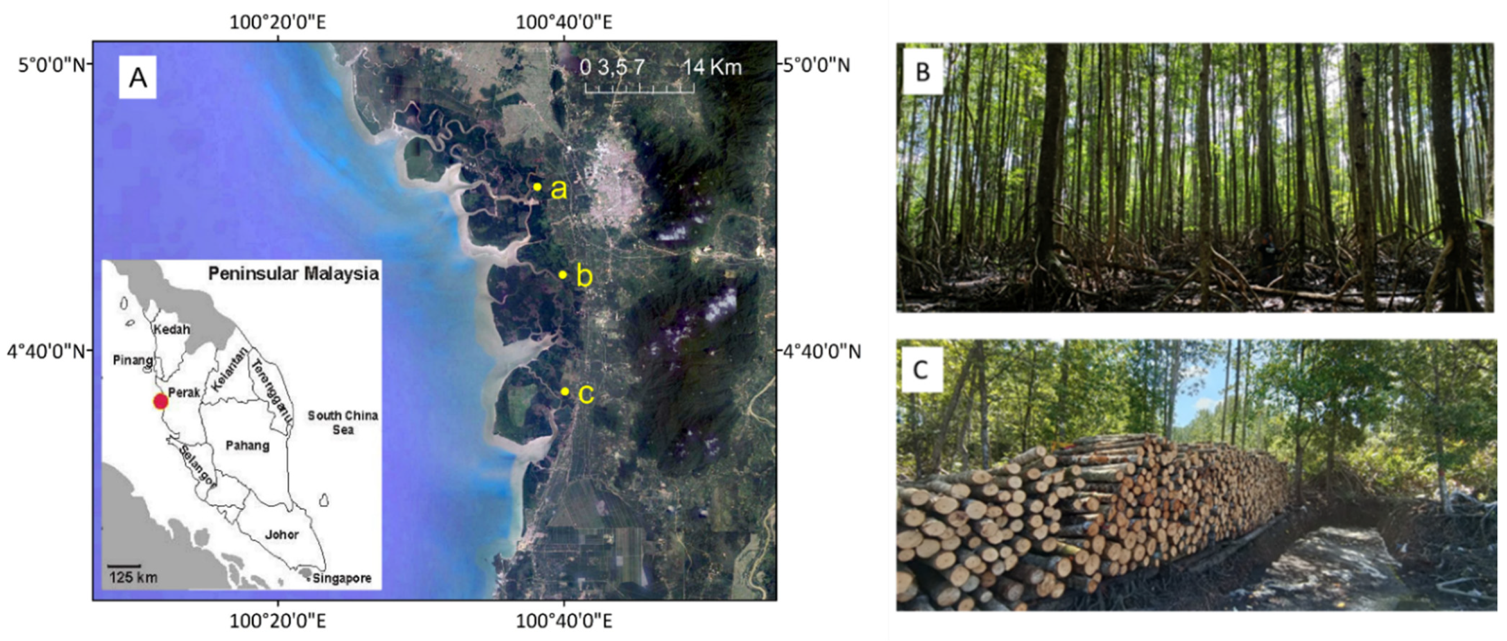
2.1. Study Area

The Matang Mangrove Forest Reserve (Figure 1) covers about 40,288 ha and has been monitored by the State Forestry Department of Perak for timber production since 1902 [25]. In 1906, it was declared a permanent forest reserve with the aim of charcoal and pole production [25]. The introduction of a new management zoning in the 2000s (management plan 2000–2009 [45]) divided the MMFR into four distinct categories: productive (74.8%), protective (17.4%), restrictive productive (6.8%), and unproductive forest (1%) [26,45,46]. While timber is extracted from the productive zone, both protective zones and restrictive zones are retained for erosion control, biodiversity preservation, preservation of the mangrove seed bank, etc. The productive zone is largely composed of mangrove stands dominated by Rhizophora species of different ages, located in 108 compartments or coupes [26,30]. According to the (2010–2019) management plan, nearly 27,430 ha were allocated for timber production; of which, 8159 ha were for the first thinning, 7678 ha were for the second thinning, and 11,593 ha were for the final felling [26]. In total, 144 charcoal contractors are present and each one is authorized to exploit 2.2 ha y⁻¹ for a kiln (maximum 3 kilns allowed for each contractor). Similarly, 70 pole contractors are present with each allowed to exploit 22.3 ha y⁻¹ [26].

2.2. Data Collection and Analysis

2.2.1. Primary Source Information

This study is a follow-up from the study by Lucas et al. [37] who utilized remote sensing imagery from the MMFR from 1988 to 2016 to evaluate the structural characteristics of the mangrove forest. These data were integrated with data from Goessens et al. [30] and Adame et al. [35] to evaluate the total carbon stock of the MMFR.

Furthermore, in order to evaluate the carbon emissions from the charcoal and pole production activities, a systematic review of primary sources (books, theses, web pages, and articles) was conducted to collect the information on carbon analytical techniques, procedures estimating different emission factors, etc. In this context, a wealth of information was extracted from the works of Satyanarayana et al. [27] along with the 2010–2019 MMFR management plan [26].

2.2.2. Vegetation Carbon Stock

To evaluate the carbon stock for the aboveground biomass (AGB) the most recent remote sensing biomass data on the productive zones in the MMFR [37] were analysed. Lucas et al. [37] estimated forest age on an annual basis for the period 1988 to 2016 by combining the time series of the Landsat-derived Normalised Difference Moisture Index (NDMI) and Japanese L-band Synthetic Aperture Radar (SAR) data. The NDMI was further used to retrieve canopy cover (%). Furthermore, interferometric Shuttle Radar Topographic Mission (SRTM) X/C-band (2000), TanDEM-X-band (2010–2016), and stereo WorldView-2 stereo (2016) data were used to estimate canopy height (CH), from which above ground biomass (AGB, Mg ha⁻¹), consisting of stem, branch, leaf biomass, and prop roots, was derived using pre-established allometry [16,34,47,48,49].

Starting from the AGB data for the year 2016 obtained from the above methods, the total AGB values (Mg) were calculated for the different zones of the MMFR. To achieve these results the age map and the biomass map were combined using QGIS to be able to differentiate the different age categories within the MMFR. The AGB data of each forest patch were subsequently multiplied by the respective area to obtain values in Mg. Finally, the biomass data were converted to carbon data with a conversion factor of 0.47 [50].

To estimate the belowground biomass (BGB), i.e., the carbon pool associated with roots, the data from Goessens et al. [30] were analysed for forest age of 15, 20, and 30 years and aboveground and belowground carbon pools were computed using the equations by Komiyama et al. [34]. The biomass values were then converted to carbon using a conversion factor of 0.39 [50]. The BGB carbon values were equivalent to ca. 35% of the aboveground values for all ages considered and hence a conversion factor of 0.35 was used to integrate the BGB carbon pool with the AGB carbon from the remote sensing data. Finally, after summing the AGB and BGB carbon values, the biomass carbon stock in the productive zones within the MMFR was mapped in QGIS according to the age of the different forest coupes.

To calculate the total carbon stock of the MMFR according to the forest zones (productive, protective, and restrictive productive), the biomass values of each single forest coupe were summed. For the protective forest zones, i.e., areas that are not used for silviculture, the AGB data were not available for most forest compartments due to the limits of the canopy height model above a certain height/age of the tree and the higher heterogeneity of the forest structure in these areas. Therefore, the biomass of a 30-year-old stand was used for the calculation of the carbon stock of the protective forest zones and the results must be considered as an underestimation of the real biomass carbon stock.

2.2.3. Soil Carbon

Soil carbon data were estimated from Adame et al. [35] who measured the carbon content in 1 m soil cores at different forest ages (5, 15, 30, and 40 years and a clear-felled site). Mean carbon values were extrapolated for ages ranging 0 to 30 years and each forest patch of a certain age was associated with its soil carbon value, using the same procedure described above for the AGB. As for the biomass carbon, a map for soil carbon was generated for the year 2016.

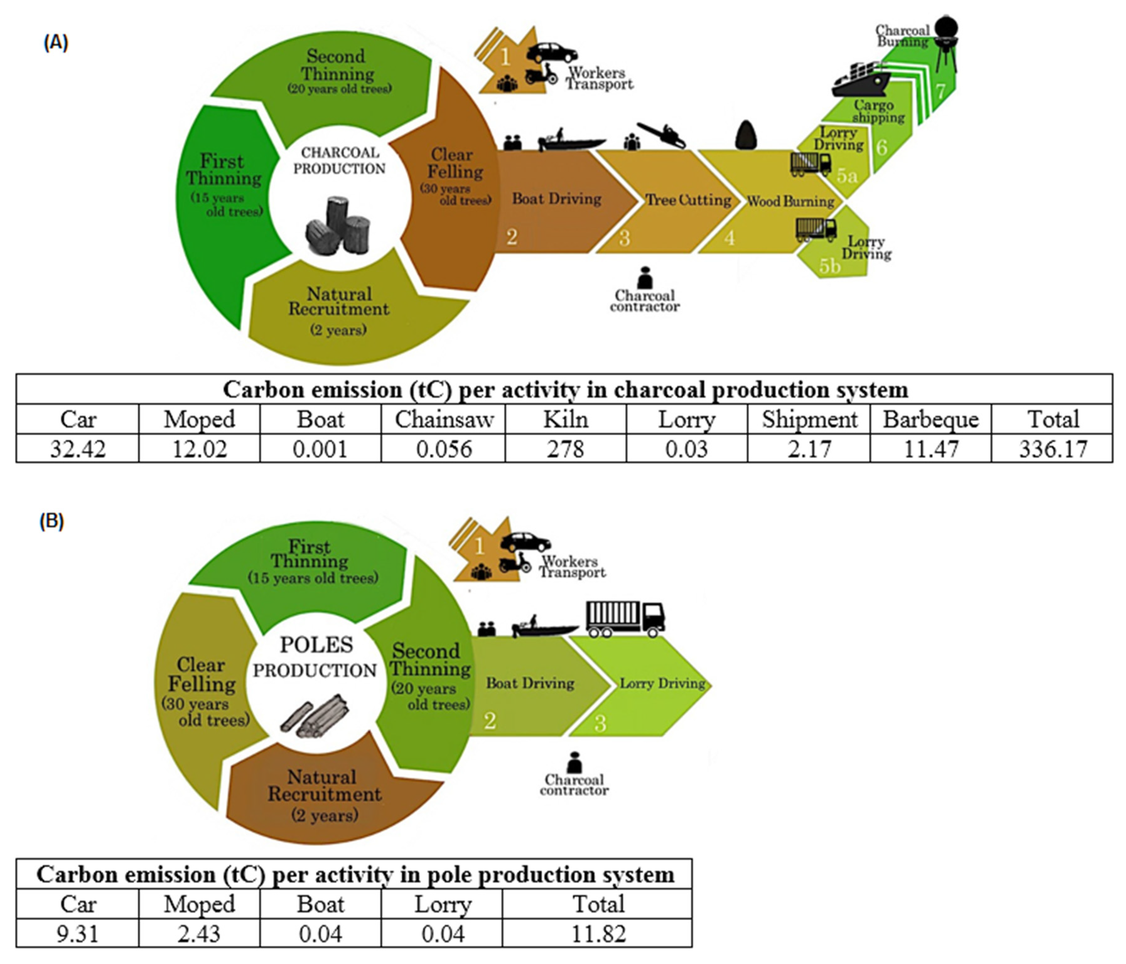
2.2.4. Carbon Emission through Charcoal and Pole Production

To estimate the carbon emissions from the silvicultural practices in the Matang Mangrove Forest Reserve, the main activities involved in mangrove charcoal and pole production systems were identified and divided into direct (i.e., activities with a direct contact with the product) and indirect tasks (i.e., out of the activity chain).

The direct tasks in charcoal production begin with transportation of tree cutters from the charcoal factory to the allocated clear-felling areas by boat. While the cutters clear fell an area of 2.2 ha of vegetation in 14 to 24 days (using chainsaw), the boat drivers transport the logs (cut into 1.6 m logs) daily to the charcoal factory. The logs are arranged inside the kilns where greenwood is converted into charcoal in 40–45 days. Nearly 80% of the charcoal from the MMFR is sent to the exporting units (by lorry) for shipment to Japan; the remaining 20% is distributed to the local markets in peninsular Malaysia [27]. Indirect tasks were represented by mode of transportation (moped or car) by the local workers to reach charcoal factories and the amount of charcoal burned for barbecuing in Japan.

In contrast to the charcoal system, mangrove pole production follows a simpler activity chain. Poles are used in peninsular Malaysia as piling material for house and road construction. Workers reach the allocated thinning areas by boat and cut down the Rhizophora trees (using an axe) by following a stick method of 1.2 m distance between the trees in 15 years and 1.8 m in 20-year-old stands. Poles are transferred to the charcoal factory by boat and from there to the local markets by lorry [27].

To estimate the carbon emissions per task/activity we referred to average emission factors that were selected based on types of equipment used and brand specifications (details can be found in the Supplementary Materials of this article). In this context, all exhaust gasses were considered and converted to carbon following the IPCC criteria [51,52]. In particular, nitrous oxide (N₂O) and methane (CH₄), though not released in large quantities, were considered after conversion to CO₂ equivalents and subsequently to carbon values. Conversion in CO₂ equivalents was conducted using the conversion factor of 21 for CH₄ and of 289.3 for N₂O and subsequently CO₂ equivalents were converted in carbon values using the conversion factor of 3.67 [51]. Emission factors for each activity, i.e., how much carbon is released during one iteration of the activity, were calculated by summing the emissions of each gas converted into carbon (Equation (1)).

$$\mathrm{EF} \left(\mathrm{g} \mathrm{C}\right)=\frac{\mathrm{C} \left(\mathrm{C}{\mathrm{O}}_2\right)}{{\mathrm{n}}_1}+\frac{\mathrm{C} \left(\mathrm{C}\mathrm{O}\right)}{{\mathrm{n}}_2}+\frac{\mathrm{C} \left(\mathrm{C}{\mathrm{H}}_4\right)}{{\mathrm{n}}_3}+\frac{\mathrm{C} \left({\mathrm{N}}_2\mathrm{O}\right)}{{\mathrm{n}}_4}$$

(1)

where C () represents the conversion of the different gasses into carbon and n₁, n₂, n₃, and n₄ represent the total emissions per each gas.

The actual carbon emission per activity (gC) was calculated by multiplying the emission factor by the corresponding distances for travelling (for boat, truck, moped, and car) and quantities of greenwood for conversion into charcoal in the kilns, and quantities of charcoal for export and use for barbecue (

Table 1. Equations used for the calculation of carbon emissions for each activity in the pole and charcoal production chain. The emission factors were computed using Equation (1).

Activity	Equation
Tree cutting	Equation (2)
Logs transport by small boat	Equation (3)
Conversion of wood into charcoal in kiln	Equation (4)
Charcoal transport by truck	Equation (5)
Charcoal transport by Cargo ship for exportation	Equation (6)
Tree cutters transport by boat	Equation (3)
Workers and contractors transport by moped	Equation (7)
Workers and contractors transport by car	Equation (8)
Barbecue	Equation (9)

). All these were calculated firstly for one iteration of each activity using Equations (2)–(9).

$$\mathrm{Total} \mathrm{C} \mathrm{emissions} \mathrm{chainsaw} \left(\mathrm{gC}\right)=a \left[{\mathrm{gC} \mathrm{Kwh}}^{-1}\right]\times b \left[\mathrm{kW}\right]\times c\left[\mathrm{h}\right]$$

(2)

where a is the carbon emission factor value, b is the unit of power from the selected chainsaw, and c is the time of use in hours.

$$\mathrm{Total} \mathrm{C} \mathrm{emissions} \mathrm{boat} \left(\mathrm{gC}\right)=a \left[{\mathrm{gCKm}}^{-1} \right]\times b \left[\mathrm{km}\right]$$

(3)

where a is the carbon emission factor value and b is the total distance in kilometres.

$$\mathrm{Total} \mathrm{C} \mathrm{emissions} \mathrm{kiln} \left(\mathrm{gC}\right)=a \left[{\mathrm{gCKg}}^{-1} \right]\times b \left[\mathrm{kg}\right]$$

(4)

where a is the carbon emission factor value and b is the amount of charcoal in grams.

$$\mathrm{Total} \mathrm{C} \mathrm{emissions} \mathrm{truck} \left(\mathrm{gC}\right)=a \left[{\mathrm{gCKm}}^{-1} \right]\times b \left[\mathrm{km}\right]$$

(5)

where a is the carbon emission factor value and b is the total distance in kilometres.

$$\mathrm{Total} \mathrm{C} \mathrm{emissions} \mathrm{Cargo} \mathrm{Ship} \left(\mathrm{gC}\right)=a \left[{\mathrm{gC} \mathrm{tKm}}^{-1} \right]\times b \left[\mathrm{Mg}\right]\times c \left[\mathrm{Km}\right]$$

(6)

where a is the carbon emission factor value, b is the amount of charcoal transported in tonnes, and c is the total distance in kilometres.

$$\mathrm{Total} \mathrm{C} \mathrm{emissions} \mathrm{moped} \left(\mathrm{gC}\right)=a \left[{\mathrm{gCKm}}^{-1} \right]\times b \left[\mathrm{km}\right]$$

(7)

where a is the carbon emission factor value and b is the total distance in kilometres.

$$\mathrm{Total} \mathrm{C} \mathrm{emissions} \mathrm{car} \left(\mathrm{gC}\right)=a \left[{\mathrm{gCKm}}^{-1} \right]\times b \left[\mathrm{km}\right]$$

(8)

where a is the carbon emission factor value and b is the total distance in kilometres.

$$\mathrm{Total} \mathrm{C} \mathrm{emissions} \mathrm{barbecue} \left(\mathrm{gC}\right)=a \left[{\mathrm{gCKg}}^{-1} \right]\times b \left[\mathrm{kg}\right]$$

(9)

where a is the carbon emission factor value and b is the total amount of charcoal in kilograms.

Due to uncertain details of the transportation used by different stakeholders in both charcoal and pole production chains, some carbon emission estimates were formed based on best professional judgment.

To calculate the total emissions for the charcoal and pole production chains, the results from the single activities were combined after multiplication by the number of iterations of each task needed to complete the production for the licensed annual area allocated to one contractor (i.e., 2.2 ha for charcoal and 22.4 ha for poles). Afterwards, the emissions were also computed for the total allocated area for charcoal and pole production reported in the latest management plan.

Additionally, carbon loss from the soil after clear-felling was also considered as a side effect of the charcoal production by referring to the findings by Adame et al. [35]. In this context, the carbon content of the upper first meter of soil from a 30-year-old stand was duly compared with a clear-felled site.

2.2.5. Comparison between Carbon Content and Carbon Emission

To evaluate whether or not the MMFR area under silvicultural management can be considered carbon neutral, the estimates of carbon sequestration and carbon emissions were duly computed. First, the emissions from pole and charcoal production were compared with the carbon stock of the productive forest and then the protective forest carbon stock was added to calculate the total carbon budget of the MMFR.

The comparison between carbon emissions and carbon stock was possible because we considered the emissions for a rotation cycle of 30 years based on the area information provided by the latest management plan [26] and we compared it with the carbon stock accumulated in the productive areas over 30 years.

3. Results

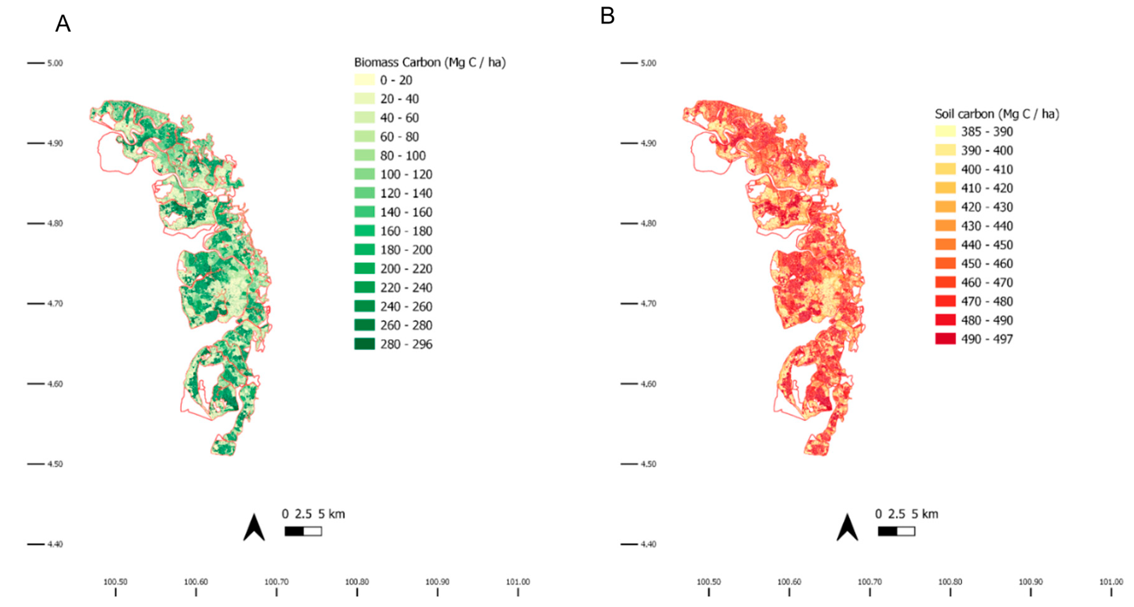
3.1. Carbon Stock in the MMFR

To classify the areas based on the rotation cycle and silvicultural thinning practice at 15 and 20 years, respectively, the productive zone was divided into three categories: 0–15 years, 16–20 years, and 21–30 years (

Table 2. Total carbon stock (C) in AGB, BGB, and top 1 m of soil for the productive, restrictive productive, and protective forest zones in the MMFR. For the protective forest the biomass and carbon per ha was considered at least equal to a 30-year-old stand, as these forest areas are in many cases older than that; hence, the values reported for the protective forest are an underestimation of the real carbon stock.

	Area (ha)	Total C AGB (Mg)	Total C BGB (Mg)	Total C Soil (Mg)
Productive forest
Age 0–15	15,170.2	552,151.6	193,253.1	6,624,517.1
Age 15–20	4435.2	384,578.1	134,602.3	2,158,387.3
Age 20–30	8786.5	465,915.5	163,070.4	3,900,523.9
TOTAL	28,391.9	1,402,645.3	490,925.8	12,683,428.4
Restrictive productive forest	2068.0	93,147.4	32,601.6	910,401.2
Protective forest	11,661.8	1,202,539.0	420,888.7	5,801,745.5
TOTAL MMFR	42,121.7	2,698,331.7	1,435,341.9	32,079,003.5

, Figure 2). The carbon stock ranged from 0 (clear-felled area) to 219.4 Mg ha⁻¹ (30-year-old stand) for the AGB and from 0 to 36.1 Mg ha⁻¹ for the BGB. Soil carbon in the top 1 m of soil had a range of 385.2 Mg ha⁻¹ to 497.5 Mg ha⁻¹ from a clear-felled area to a 30-year-old site (Figure 3). Considering these values, the total carbon stock in the biomass for the productive forest was equal to 1,893,571.1 Mg C, while the total for the protective forest was at least equal to 1,623,427.7 Mg C. Regarding the soil carbon pool, this was equal to 12,683,428.4 Mg C and 5,801,745.5 Mg C for the productive forest and the protective forest, respectively.

Considering the total areas occupied by different forest zones (productive, restrictive productive, and protective), the total C stock for the MMFR (AGB, BGB, and soil combined) would be equal to 36,212,677.1 Mg C.

3.2. Carbon Emissions Factors from Charcoal and Pole Production

For the production of charcoal, transportation of people/logs in the boats had the minimum average carbon emission factors (1.14 g C km⁻¹), while greenwood conversion into charcoal showed the maximum (702 g C kg⁻¹) (

Table 3. Average carbon emission factors per each activity in the two production chains (charcoal and poles). These values were calculated considering the brands and models of the equipment used, number of workers, and mean distances travelled.

			Average Carbon Emissions Factors
Type of Activity	Material Used	Units	Charcoal Production Chain	Poles Production Chain
Boat driving	Small boat	g C Km−1	1.14	1.16
Tree cutting	Chainsaw	g C kWh	350.00	-
Wood burning	Kiln	g C Kg−1	702.03	-
Log transportation	Container truck	g C Km−1	220.37	-
	General truck	g C Km−1	-	167.45
Worker’s transportation	car	g C Km−1	42.83	42.83
	moped	g C Km−1	18.01	18.01
Cargo shipping	Cargo ship	g C t-Km−1	4.16	-
Charcoal burning	barbecue	g C Kg−1	139.78	-

). In the case of mangrove pole production, transport by boats had the lowest carbon emission factor (1.16 g C km⁻¹) whereas transport by lorries distributing poles to local markets had the highest (167.45 g C km⁻¹) (Table 3).

3.2.1. Carbon Emission from the Areas Assigned to One Contractor

The area of 2.2 ha allocated for charcoal production in a year provides an average yield of 396 Mg (i.e., 180 Mg ha⁻¹). According to the management plan, 40.8 Mg of greenwood (with additional 12.2 Mg as firing material) is required per kiln to produce 11 Mg of charcoal in 40–45 days. On this basis, 304.85 Mg out of 396 Mg greenwood in 2.2 ha is used for charcoal production and 91.15 Mg as firewood which ultimately delivers 82.08 Mg of charcoal. After considering the amount of wood used in charcoal production and its yield, along with the number of workers involved and the kilometres travelled for transport, the carbon emission estimates were found to be ranging from 0.001 Mg C for boat transport to 278 Mg C for greenwood burning inside the kilns for a total of 336.17 Mg C (Figure 4). Likewise, the pole production from a 22.3 ha area of intermediate thinning, together with average number of workers involved in the different activities, amounted to carbon emission ranging from 0.04 Mg C for boat/lorry transports to 9.31 Mg C for car transport, for a total of 11.82 Mg C (Figure 4).

3.2.2. Carbon Emission from the Total Areas of Pole and Charcoal Production

Dividing the emissions for the area assigned to one contractor by the area in hectares, the carbon emission factor per ha would be equal to 152.8 Mg C/ha for charcoal production and 0.53 Mg C ha⁻¹ for pole production.

Considering the total areas for thinning I and II and clear-felling reported by the latest management plan of 2010–2019 [26] equal to 8159 ha, 7678 ha, and 11,593 ha, respectively (named as allocated areas in

Table 4. Comparison between carbon stock in the vegetation biomass and carbon emissions over a period of 30 years for the productive forest in the MMFR. For the carbon stock, the values were calculated based on 15-, 20- and 30-year-old forest stands AGB values (163.5 Mg ha⁻¹, 190.5 Mg ha⁻¹, 219.4 Mg ha⁻¹, respectively) following the age of thinning and clear-felling reported by the last management plan.

	Biomass Carbon Stock (Mg)		Carbon Emissions (Mg)
	Licenced * Area	Allocated * Area	Licenced Area	Allocated Area
Thinning I	1713.64	626,978.35	11.82	4324.63
Thinning II	1996.63	687,449.73	11.82	4069.68
Clear-felling	226.86	1,195,446.97	336.17	1,771,463.09

* Licensed area = 2.2 ha for charcoal and 22.3 ha for poles. * Allocated area = total area reported by the current management plan for felling (8159 and 7678 ha for first and second thinning, respectively, and 11,593 ha for final felling).

), the total emissions are of 4.32 Gg C for pole production from thinning I, 8.13 Gg C for pole production from thinning I and 1.77 Tg C for charcoal production.

3.2.3. Carbon Loss from Soil after Clear-Felling

Based on the data of Adame et al. [35], the carbon loss from the soil due to clear-felling activities was also calculated. On average, the carbon stock in the soil of a clear-felled site is 385.2 Mg C ha⁻¹, while a 30-year-old site has a carbon stock of 497.5 Mg C ha⁻¹. Consequently, there is a loss of 112.3 Mg C ha⁻¹ each time an area is cleared for charcoal production. By considering the total area assigned for clear-felling in the 2010–2019 management plan (11,593 ha), the total carbon loss from the soil would be equal to 1,301,893.9 Mg C.

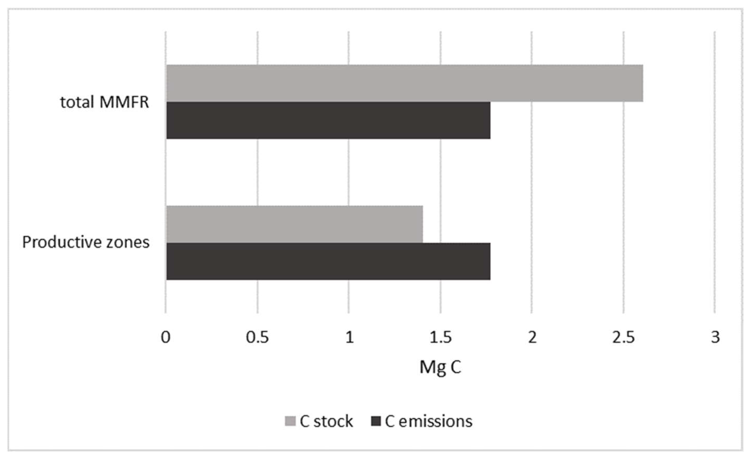
3.3. Carbon Stock Versus Carbon Emission

The biomass carbon stock was compared with the carbon emissions considering the emissions due to the activities practiced during the first and second thinning (pole production) and clear-felling (charcoal production), as well as the carbon loss from the soil after clear-felling (Table 4). For a licensed area assigned to one contractor, i.e., 22.3 ha for thinnings and 2.2 ha for clear-felling, the emissions are much lower for the pole production compared with the charcoal production. On the other hand, in the case of a clear-felling area, the emissions are higher compared with the biomass carbon stock.

The carbon budget of the productive forest was computed taking into account the areas allocated for poles and charcoal reported in the latest management plan and their derived emission values together with the vegetation carbon stock calculated from the remote sensing data. The AGB carbon stock of the productive forest alone, equal to 1,402,645.3 Mg C (Table 1) was compared with the emissions of 1,771,463.09 Mg C (Table 4). Hence, the carbon budget of the silvicultural activities were negative (−381,228.1 Mg C) (Figure 5). Considering the total area of the MMFR, i.e., including protective and restrictive productive zones, the total carbon stock was equal to 2,698,331.7 Mg C (Table 1), which compared with the emission values reported above, resulted in a positive carbon budget (+341,113.4 Mg C) (Figure 5).

Moreover, if we also consider the soil carbon, the total carbon stock of the productive zones of the MMFR would be equal to 14,576,999.5 Mg C. On the same line, the total emissions, including the carbon loss from the soil, would be equal to 3,073,357.0 Mg C. This was not included in the budget calculation as the carbon in the soil accumulates over time and cannot be compared with the emissions of a thirty-year cycle.

4. Discussion

4.1. Vegetation Biomass and Soil Carbon Stock

Given the key role of mangroves as carbon stock, we measured the carbon sequestration potential of MMFR, and subsequently compared this with the C emissions originating from pole and charcoal production. The total carbon in the soil was also evaluated to provide an overview of the total carbon stock of the MMFR.

Regarding the vegetation biomass, remote sensing data are a valuable source for biomass estimations in mangroves and can provide a very detailed view of an area over time [37,38]. Furthermore, we integrated data from field measurements [30,35] with the age maps obtained through remote sensing [37], producing for the first time an accurate representation of the carbon storage in the entire MMFR that includes not only vegetation but also the belowground component (i.e., roots and soil).

In this study the carbon stock of the MMFR was firstly calculated based on AGB data derived from remote sensing analysis. The main advantage of the use of remote sensing data in this study is that each forest coupe was considered with its own age and biomass values whereas previous biomass estimations were based on field data collection alone (e.g., Goessens et al. [30]) and could not provide an estimate for the entire forest as only specific forest ages were selected for the study (namely 15-, 20-, 30-year-old and protective forest). Thus, our results should provide a more reliable overview of the carbon stored in the MMFR. Furthermore, to have a complete understanding of the carbon stored in the ecosystem, other components such as belowground and soil carbon, which are often overlooked when only remote sensing data are used, were considered. Previous studies [8,35,53,54,55,56,57] all reported the importance of belowground carbon which is considered to store from 50 to 90% [50] of the total mangrove ecosystem carbon stock. Until now the only study in the MMFR that measured soil carbon in the soil was Adame et al. [35] and their estimates ranged (approximately) from 380 Mg C ha⁻¹ for a 1-year-old forest to 480 Mg C ha⁻¹ for a 30-year-old forest and reached 540 Mg C ha⁻¹ in the protective forest (for the first meter of soil). By extrapolating soil carbon values for all forest ages and linking them to the areal extent of each forest zone, we estimated that the total carbon storage in the soil can reach 31,637,347.8 Mg C. Hence the carbon storage in the soil seems to be much greater than the carbon stock in the vegetation biomass, with this estimated to be 2,698,331.7 Mg C.

However, the above estimates only consider the carbon in the soil in the first 1 m while it is known that mangrove soils can be much deeper than 1 m [50]. Thus, further research should be focused on deeper soil layers to obtain a more accurate representation of the carbon stock in the mangrove forest.

4.2. Charcoal and Pole Production Chains: Carbon Emissions

The different emissions in the two production chains were expected considering the difference in the number of activities and workers involved in each type of production, with total carbon emission values of 11.82 Mg C on average for pole production and a total average of 336.17 Mg C for charcoal production per licensed area. In other words, pole production in MMFR was found to release on average 84% less carbon than charcoal production.

Nevertheless, during our calculations of emissions in the various stages of the production chains, we noticed a lack of easily available specific information (e.g., regarding the mode of transport used, chainsaw brand, and specific number of users). For wood burning, other research studies such as Lacaux et al. [41], Kridiborwnorn et al. [43] and Sparrevik et al. [58] used a complex experimental design by considering more detailed values (e.g., wood carbon (%), wood calorific value (kJ/g), brands carbon (%)) with more comprehensive and complete results. At the same time, information about exhaust emission released by transports was limited or difficult to follow because of the need for specific data that were unavailable for our study. Moreover, the other factors such as the local guards’ role, which involves use of the boats to monitor the productive area, and the activities linked to mangroves replanting with seedlings were not considered in the present study due to lack of information.

4.3. Vegetation Carbon Stock Versus Carbon Emissions

A comparison between the values for carbon sequestration and carbon emissions at MMFR was conducted taking into account the different areas of exploitation. Considering the biomass carbon stock in the productive area compared with the emissions from the pole and charcoal production for a thirty-year cycle, the emissions were estimated to be greater than the carbon stock. This is because the activities included in the production chain also use fuels other than mangrove wood, making the budget negative. If the forest was used entirely for charcoal production, the management would be unsustainable from a carbon point of view. Furthermore, if we also include the emissions from the soil after clear-felling calculated by Adame et al. [35] who estimated a drop of 43% in soil carbon after clearing, the emissions would be even higher.

In order to achieve carbon neutrality for the productive forest, it is necessary to reduce the area allocated for clear-felling by at least 20.8%, implying a reduction in the productive forest from 74.8% to 45.6% of the entire MMFR. Fortunately, even in the current situation, the MMFR also includes areas that are not exploited and are left unmanaged (i.e., protective forest zones) that can compensate for the loss of carbon from the productive zones. When the carbon stock of these areas was considered into the carbon budget, it was positive, providing the management a more sustainable outlook. However, the current management does not take into account possible disruptions caused by climate change (e.g., rising sea levels and increased storm intensity), that can affect the yield and functionality of the mangrove forest.

Given the importance of carbon sequestration for climate change mitigation, it would be better for the MMFR to increase the protective zone areas and REDD+ or similar projects can be considered as an alternative source of income, as already suggested by other studies [35,59].

On the contrary, in recent years an increase in exploitation of the restrictive productive zones has been observed (Harry Yong, personal communication, June 2019), probably due to the decrease in yield caused by mangrove degradation [60] and the parallel high demand for charcoal, leading to more clear-felling activities and subsequently higher emissions. This is concerning as the MMFR seems to slowly become more unsustainable in its silvicultural practices.

5. Conclusions

The present study provided valuable information regarding the emissions released by pole and charcoal production in the MMFR. By using the most recent biomass and carbon data we provided an accurate overview of the detailed carbon stock in MMFR and for the first time this was integrated with emission estimates caused by charcoal and pole production. Therefore, this study can be used as a pilot project to evaluate similar silvicultural mangrove management schemes worldwide.

At the carbon sequestration side, many unknowns remain, particularly regarding the depth of soils under mangroves and the actual carbon stock belowground together with how the thinning process, the clear cutting, and the replanting stages influence the carbon cycle dynamics. Furthermore, data on other ecosystem components such as leaf litter, dead wood, and fauna is very limited.

In general, considering the values obtained in this study, we can conclude that the total area of the MMFR can be considered carbon positive, despite the emissions caused by the silvicultural activities. However, we suggest a reduction in the productive zones of at least 20% to achieve carbon neutrality in the productive forest coupes.

This exploratory study helps to strengthen the assumption that the protection of mangrove forest must be a priority as they are among some of the carbon-richest ecosystems in the world. We also show that a sustainable exploitation of mangroves for pole and charcoal production is possible from a carbon point of view if the exploited area is managed properly. In this way mangroves can continue to be an excellent carbon stock and the livelihood of local people that depend on this ecosystem can be sustained.

References

1. Sivakumar, M.V.K.; Stefanski, R. Climate Change in South Asia. In Climate Change and Food Security in South Asia; Lal, R., Sivakumar, M.V.K., Faiz, S.M.A., Mustafizur Rahman, A.H.M., Islam, K.R., Eds.; Springer: Dordrecht, The Netherlands, 2011; pp. 13–30. [Google Scholar] [CrossRef]
2. Satyanarayana, B.; Van der Stocken, T.; Rans, G.; Kodikara, K.A.S.; Ronsmans, G.; Jayatissa, L.P.; Husain, M.-L.; Koedam, N.; Dahdouh-Guebas, F. Island-wide coastal vulnerability assessment of Sri Lanka reveals that sand dunes, planted trees and natural vegetation may play a role as potential barriers against ocean surges. Glob. Ecol. Conserv. 2017, 12, 144–157. [Google Scholar] [CrossRef]
3. Stocker, T.F.; Qin, D.; Plattner, G.K.; Tignor, M.; Allen, S.K.; Boschung, J.; Midgley, B.M. IPCC, 2013: Climate Change 2013: The Physical Science Basis. Contribution of Working Group I to the Fifth Assessment Report of the Intergovernmental Panel on Climate Change; Cambridge University Press: Cambridge, UK, 2013. [Google Scholar]
4. Pearson, T.R.H.; Brown, S.; Casarim, F.M. Carbon emissions from tropical forest degradation caused by logging. Environ. Res. Lett. 2014, 9, 034017. [Google Scholar] [CrossRef] [Green Version]
5. Ahmed, N.; Glaser, M. Coastal aquaculture, mangrove deforestation and blue carbon emissions: Is REDD+ a solution? Mar. Policy 2016, 66, 58–66. [Google Scholar] [CrossRef]
6. Twilley, R.R.; Chen, R.H.; Hargis, T. Carbon sinks in mangroves and their implications to carbon budget of tropical coastal ecosystems. Water Air Soil Pollut. 1992, 64, 265–288. [Google Scholar] [CrossRef]
7. Bouillon, S.; Borges, A.V.; Castaneda, E.; Diele, K.; Dittmar, T.; Duke, N.C.; Kristensen, E.; Lee, S.Y.; Marchand, C.; Middelburg, J.; et al. Mangrove production and carbon sinks: A revision of global budget estimates. Glob. Biogeochem. Cycles 2008, 22, 2. [Google Scholar] [CrossRef] [Green Version]
8. Macreadie, P.I.; Anton, A.; Raven, J.A.; Beaumont, N.; Connolly, R.M.; Friess, D.A.; Kelleway, J.J.; Kennedy, H.; Kuwae, T.; Lavery, P.S.; et al. The future of Blue Carbon science. Nat. Commun. 2019, 10, 3998. [Google Scholar] [CrossRef] [Green Version]
9. Du Pont, Y.R.; Jeffery, M.L.; Gütschow, J.; Rogelj, J.; Christoff, P.; Meinshausen, M. Equitable mitigation to achieve the Paris Agreement goals. Nat. Clim. Chang. 2017, 7, 38–43. [Google Scholar] [CrossRef] [Green Version]
10. Hamilton, S.E.; Friess, D.A. Global carbon stocks and potential emissions due to mangrove deforestation from 2000 to 2012. Nat. Clim. Chang. 2018, 8, 240–244. [Google Scholar] [CrossRef] [Green Version]
11. Macreadie, P.I.; Costa, M.D.P.; Atwood, T.B.; Friess, D.A.; Kelleway, J.J.; Kennedy, H.; Lovelock, C.E.; Serrano, O.; Duarte, C.M. Blue carbon as a natural climate solution. Nat. Rev. Earth Environ. 2021, 2, 826–839. [Google Scholar] [CrossRef]
12. Aziz, A.A.; Thomas, S.; Dargusch, P.; Phinn, S. Assessing the potential of REDD+ in a production mangrove forest in Malaysia using stakeholder analysis and ecosystem services mapping. Mar. Policy 2016, 74, 6–17. [Google Scholar] [CrossRef]
13. Donato, D.C.; Kauffman, J.B.; Murdiyarso, D.; Kurnianto, S.; Stidham, M.; Kanninen, M. Mangroves among the most carbon-rich forests in the tropics. Nat. Geosci. 2011, 4, 293–297. [Google Scholar] [CrossRef]
14. Rovai, A.S.; Twilley, R.R.; Castaneda, E.; Riul, P.; Cifuentes-Jara, M.; Manrow-Villalobos, M.; Horta, P.A.; Simonassi, J.C.; Fonseca, A.L.D.O.; Pagliosa, P. Global controls on carbon storage in mangrove soils. Nat. Clim. Chang. 2018, 8, 534–538. [Google Scholar] [CrossRef]
15. Sanderman, J.; Hengl, T.; Fiske, G.; Solvik, K.; Adame, M.F.; Benson, L.; Bukoski, J.J.; Carnell, P.; Cifuentes-Jara, M.; Donato, D.; et al. A global map of mangrove forest soil carbon at 30 m spatial resolution. Environ. Res. Lett. 2018, 13, 055002. [Google Scholar] [CrossRef]
16. Simard, M.; Fatoyinbo, L.; Smetanka, C.; Rivera-Monroy, V.H.; Castañeda-Moya, E.; Thomas, N.; Van Der Stocken, T. Mangrove canopy height globally related to precipitation, temperature and cyclone frequency. Nat. Geosci. 2019, 12, 40–45. [Google Scholar] [CrossRef]
17. Kauffman, J.B.; Adame, M.F.; Arifanti, V.B.; Schile-Beers, L.M.; Bernardino, A.F.; Bhomia, R.K.; Donato, D.C.; Feller, I.C.; Ferreira, T.O.; Garcia, M.D.C.J.; et al. Total ecosystem carbon stocks of mangroves across broad global environmental and physical gradients. Ecol. Monogr. 2020, 90, e01405. [Google Scholar] [CrossRef] [Green Version]
18. Sasmito, S.D.; Taillardat, P.; Clendenning, J.N.; Cameron, C.; Friess, D.A.; Murdiyarso, D.; Hutley, L.B. Effect of land-use and land-cover change on mangrove blue carbon: A systematic review. Glob. Chang. Biol. 2019, 25, 4291–4302. [Google Scholar] [CrossRef]
19. Adame, M.F.; Connolly, R.M.; Turschwell, M.P.; Lovelock, C.E.; Fatoyinbo, T.; Lagomasino, D.; Goldberg, L.A.; Holdorf, J.; Friess, D.A.; Sasmito, S.D.; et al. Future carbon emissions from global mangrove forest loss. Glob. Chang. Biol. 2021, 27, 2856–2866. [Google Scholar] [CrossRef]
20. Richards, D.R.; Friess, D.A. Rates and drivers of mangrove deforestation in Southeast Asia, 2000–2012. Proc. Natl. Acad. Sci. USA 2016, 113, 344–349. [Google Scholar] [CrossRef] [Green Version]
21. Chatting, M.; Al-Maslamani, I.; Walton, M.; Skov, M.W.; Kennedy, H.; Husrevoglu, Y.S.; Le Vay, L. Future Mangrove Carbon Storage Under Climate Change and Deforestation. Front. Mar. Sci. 2022, 9, 781876. [Google Scholar] [CrossRef]
22. Hansen, M.C.; Stehman, S.V.; Potapov, P.V. Quantification of global gross forest cover loss. Proc. Natl. Acad. Sci. USA 2010, 107, 8650–8655. [Google Scholar] [CrossRef] [Green Version]
23. Zhila, H.; Mahmood, H.; Rozainah, M.Z. Biodiversity and biomass of a natural and degraded mangrove forest of Peninsular Malaysia. Environ. Earth Sci. 2014, 71, 4629–4635. [Google Scholar] [CrossRef]
24. Gopalakrishnan, L.; Satyanarayana, B.; Chen, D.; Wolswijk, G.; Amir, A.A.; Vandegehuchte, M.B.; Muslim, A.B.; Koedam, N.; Dahdouh-Guebas, F. Using Historical Archives and Landsat Imagery to Explore Changes in the Mangrove Cover of Peninsular Malaysia between 1853 and 2018. Remote Sens. 2021, 13, 3403. [Google Scholar] [CrossRef]
25. Noakes, D.S.P. A Working plan for the Matang Mangrove Forest Reserve Perak; Forest Department, Federation of Malaya: Kuala Lumpur, Malaysia, 1952; p. 173. [Google Scholar]
26. Arifin, R.; Mustafa, N.M.S.N. A Working Plan for the Matang Mangrove Forest Reserve, Perak, 6th ed.; State Forestry Department: Ipoh, Malaysia, 2013. [Google Scholar]
27. Satyanarayana, B.; Quispe-Zuniga, M.R.; Hugé, J.; Sulong, I.; Mohd-Lokman, H.; Dahdouh-Guebas, F. Mangroves Fueling Livelihoods: A Socio-Economic Stakeholder Analysis of the Charcoal and Pole Production Systems in the World’s Longest Managed Mangrove Forest. Front. Ecol. Evol. 2021, 9, 621721. [Google Scholar] [CrossRef]
28. Ong, J.E.; Gong, W.K.; Wong, C.H. Seven Years of Productivity Studies in a Malaysian Managed Mangrove Forest then What. Coasts and Tidal Wetlands of the Australian Monsoon Region; Australian National University: Canberra, ACT, Australia, 1985; pp. 213–223. [Google Scholar]
29. Putz, F.E.; Chan, H.T. Tree growth, dynamics, and productivity in a mature mangrove forest in Malaysia. For. Ecol. Manag. 1986, 17, 211–230. [Google Scholar] [CrossRef]
30. Goessens, A.; Satyanarayana, B.; Van der Stocken, T.; Quispe-Zuniga, M.R.; Mohd-Lokman, H.; Sulong, I.; Dahdouh-Guebas, F. Is Matang Mangrove Forest in Malaysia Sustainably Rejuvenating after More than a Century of Conservation and Harvesting Management? PLoS ONE 2014, 9, e105069. [Google Scholar] [CrossRef]
31. Otero, V.; Van De Kerchove, R.; Satyanarayana, B.; Martínez-Espinosa, C.; Fisol, M.A.B.; Ibrahim, M.R.B.; Sulong, I.; Mohd-Lokman, H.; Lucas, R.; Dahdouh-Guebas, F. Managing mangrove forests from the sky: Forest inventory using field data and Unmanned Aerial Vehicle (UAV) imagery in the Matang Mangrove Forest Reserve, peninsular Malaysia. For. Ecol. Manag. 2018, 411, 35–45. [Google Scholar] [CrossRef]
32. Ong, J.E.; Gong, W.K.; Wong, C.H. Allometry and partitioning of the mangrove, Rhizophora apiculata. For. Ecol. Manag. 2005, 188, 395–408. [Google Scholar] [CrossRef]
33. Komiyama, A.; Poungparn, S.; Kato, S. Common allometric equations for estimating the tree weight of mangroves. J. Trop. Ecol. 2005, 21, 471–477. [Google Scholar] [CrossRef]
34. Komiyama, A.; Ong, J.E.; Poungparn, S. Allometry, biomass, and productivity of mangrove forests: A review. Aquat. Bot. 2008, 89, 128–137. [Google Scholar] [CrossRef]
35. Adame, M.; Zakaria, R.; Fry, B.; Chong, V.; Then, Y.; Brown, C.; Lee, S.Y. Loss and recovery of carbon and nitrogen after mangrove clearing. Ocean Coast. Manag. 2018, 161, 117–126. [Google Scholar] [CrossRef]
36. Otero, V.; Van De Kerchove, R.; Satyanarayana, B.; Mohd-Lokman, H.; Lucas, R.; Dahdouh-Guebas, F. An Analysis of the Early Regeneration of Mangrove Forests using Landsat Time Series in the Matang Mangrove Forest Reserve, Peninsular Malaysia. Remote Sens. 2019, 11, 774. [Google Scholar] [CrossRef] [Green Version]
37. Lucas, R.; Van De Kerchove, R.; Otero, V.; Lagomasino, D.; Fatoyinbo, L.; Omar, H.; Satyanarayana, B.; Dahdouh-Guebas, F. Structural characterisation of mangrove forests achieved through combining multiple sources of remote sensing data. Remote Sens. Environ. 2020, 237, 111543. [Google Scholar] [CrossRef]
38. Lucas, R.; Otero, V.; Van De Kerchove, R.; Lagomasino, D.; Satyanarayana, B.; Fatoyinbo, T.; Dahdouh-Guebas, F. Monitoring Matang’s Mangroves in Peninsular Malaysia through Earth observations: A globally relevant approach. Land Degrad. Dev. 2021, 32, 354–373. [Google Scholar] [CrossRef]
39. Feldpausch, T.R.; Jirka, S.; Passos, C.A.; Jasper, F.; Riha, S.J. When big trees fall: Damage and carbon export by reduced impact logging in southern Amazonia. For. Ecol. Manag. 2005, 219, 199–215. [Google Scholar] [CrossRef]
40. Medjibe, V.P.; Putz, F.E.; Starkey, M.P.; Ndouna, A.A.; Memiaghe, H.R. Impacts of selective logging on above-ground forest biomass in the Monts de Cristal in Gabon. For. Ecol. Manag. 2011, 262, 1799–1806. [Google Scholar] [CrossRef]
41. Lacaux, J.-P.; Brocard, D.; Lacaux, C.; Delmas, R.; Brou, A.; Yoboué, V.; Koffi, M. Traditional charcoal making: An important source of atmospheric pollution in the African Tropics. Atmos. Res. 1994, 35, 71–76. [Google Scholar] [CrossRef]
42. Pennise, D.M.; Smith, K.R.; Kithinji, J.P.; Rezende, M.E.; Raad, T.J.; Zhang, J.; Fan, C. Emissions of greenhouse gases and other airborne pollutants from charcoal making in Kenya and Brazil. J. Geophys. Res. Earth Surf. 2001, 106, 24143–24155. [Google Scholar] [CrossRef] [Green Version]
43. Kridiborworn, P.; Chidthaisong, A.; Yuttitham, M.; Tripetchkul, S. Carbon sequestration by mangrove forest planted specifically for charcoal production in Yeesarn, Samut Songkram. J. Sustain. Energy Environ. 2012, 3, 87–92. [Google Scholar]
44. Bailis, R.; Rujanavech, C.; Dwivedi, P.; Vilela, A.D.O.; Chang, H.; de Miranda, R.C. Innovation in charcoal production: A comparative life-cycle assessment of two kiln technologies in Brazil. Energy Sustain. Dev. 2013, 17, 189–200. [Google Scholar] [CrossRef]
45. Muda, A.; Mustafa, N.M.S.N. A Working Plan for the Matang Mangrove Forest Reserve, Perak, 5th ed.; State Forestry Department: Ipoh, Malaysia, 2003. [Google Scholar]
46. Aziz, A.A.; Dargusch, P.; Phinn, S.; Ward, A. Using REDD+ to balance timber production with conservation objectives in a mangrove forest in Malaysia. Ecol. Econ. 2015, 120, 108–116. [Google Scholar] [CrossRef]
47. Fatoyinbo, T.; Feliciano, E.A.; Lagomasino, D.; Lee, S.K.; Trettin, C. Estimating mangrove aboveground biomass from airborne LiDAR data: A case study from the Zambezi River delta. Environ. Res. Lett. 2017, 13, 025012. [Google Scholar] [CrossRef] [Green Version]
48. Njana, M.A.; Eid, T.; Zahabu, E.; Malimbwi, R. Procedures for quantification of belowground biomass of three mangrove tree species. Wetl. Ecol. Manag. 2015, 23, 749–764. [Google Scholar] [CrossRef]
49. Chave, J.; Andalo, C.; Brown, S.; Cairns, M.A.; Chambers, J.Q.; Eamus, D.; Fölster, H.; Fromard, F.; Higuchi, N.; Kira, T.; et al. Tree allometry and improved estimation of carbon stocks and balance in tropical forests. Oecologia 2005, 145, 87–99. [Google Scholar] [CrossRef] [PubMed]
50. Kauffman, J.B.; Donato, D. Protocols for the Measurement, Monitoring and Reporting of Structure, Biomass and Carbon Stocks in Mangrove Forests; No. CIFOR Working Paper no. 86, p. 40p; Center for International Forestry Research (CIFOR): Bogor, Indonesia, 2012; 40p. [Google Scholar]
51. IPCC—Intergovernmental Panel on Climate Change. 2006 IPCC Guidelines for National Greenhouse Gas Inventories; IPCC: Geneva, Switzerland, 2006. [Google Scholar]
52. IPCC—Intergovernmental Panel on Climate Change. 2019 Refinement to the 2006 IPCC Guidelines for National Greenhouse Gas Inventories; IPCC: Geneva, Switzerland, 2019. [Google Scholar]
53. Bouillon, S. Storage beneath mangroves. Nat. Geosci. 2011, 4, 282. [Google Scholar] [CrossRef] [Green Version]
54. Alongi, D.M. Carbon Cycling and Storage in Mangrove Forests. Annu. Rev. Mar. Sci. 2014, 6, 195–219. [Google Scholar] [CrossRef]
55. Kauffman, J.B.; Heider, C.; Cole, T.G.; Dwire, K.A.; Donato, D.C. Ecosystem Carbon Stocks of Micronesian Mangrove Forests. Wetlands 2011, 31, 343–352. [Google Scholar] [CrossRef]
56. Castillo, J.A.A.; Apan, A.A.; Maraseni, T.N.; Salmo, S.G. Soil C quantities of mangrove forests, their competing land uses, and their spatial distribution in the coast of Honda Bay, Philippines. Geoderma 2017, 293, 82–90. [Google Scholar] [CrossRef]
57. Alongi, D.M. Global Significance of Mangrove Blue Carbon in Climate Change Mitigation. Science 2020, 2, 67. [Google Scholar] [CrossRef]
58. Sparrevik, M.; Adam, C.; Martinsen, V.; Jubaedah; Cornelissen, G. Emissions of gases and particles from charcoal/biochar production in rural areas using medium-sized traditional and improved “retort” kilns. Biomass-Bioenergy 2015, 72, 65–73. [Google Scholar] [CrossRef]
59. Ammar, A.A.; Dargusch, P.; Shamsudin, I. Can the Matang Mangrove Forest Reserve provide perfect teething ground for a blue carbon based REDD+ pilot project? J. Trop. For. Sci. 2014, 26, 371–381. Available online: https://www.jstor.org/stable/43150919 (accessed on 1 February 2020).
60. Hamdan, O.; Khairunnisa, M.R.; Ammar, A.A.; Hasmadi, I.M.; Aziz, H.K. Mangrove carbon stock as-sessment by optical satellite imagery. J. Trop. For. Sci. 2013, 554–565. Available online: https://www.jstor.org/stable/23616997 (accessed on 2 February 2016).
61. Husqvarna. Japan. 2017. Available online: http://www.husqvarna.com/jp/ (accessed on 1 February 2020).
62. Yanmar. Sailboat and Small Craft Engines. 2017. Available online: http://www.yanmarmarine.com/Products/Sailboat-and-small-craft-eng (accessed on 1 February 2020).
63. Gencat. Guia pràctica per al càlcul d’emissions de gasos amb efecte d’hivernacle (GEH) Versio 2016.3. Generalitat de Catalunya, Oficina del canvi climàtic. 2017. Available online: http://canviclimatic.gencat.cat/web/.content/home (accessed on 1 February 2020).
64. Distance Calculator. 2017. Available online: https://www.distancecalculator.net/ (accessed on 1 February 2020).
65. Sea Rates. 2017. Available online: https://www.searates.com/reference/portdistance/? (accessed on 1 February 2020).
66. OOCL. Environmental Care. OOCL Carbon Calculator. 2017. Available online: http://www.oocl.com/eng/aboutoocl/Environmentalcare/ooclcarboncalculator/Pages/default.Aspx (accessed on 1 February 2020).
67. Cefic. Guidelines for measuring and managing CO2 emissions from Freight Transport Operations. 2011. Available online: http://www.cefic.org/Industry-support/Responsible-CaretoolsSMEs/5-Environment/Guidelines-for-managing-CO2-emissions-fromtransportoperations/redueix_emissions/guia_de_calcul_demissions_de_co2/160411_Guia-practica-calcul-emissions_sensecanvis_CA.pdf (accessed on 1 February 2020).
68. Sea-Distances. Online Tool for Calculation Distance between Sea Ports. 2017. Available online: https://sea-distances.org (accessed on 1 February 2020).
69. Huang, H.L.; Lee, W.M.G.; Wu, F.S. Emissions of air pollutants from indoor charcoal barbecue. J. Hazard. Mater. 2016, 302, 198–207. [Google Scholar] [CrossRef] [PubMed]
70. Buhaug, Ø.; Corbett, J.J.; Endresen, O.; Eyring, V.; Faber, J.; Hanayama, S.; Lee, D.; Lindstad, H.; Mjelde, A.; Palsson, C.; et al. Second IMO Greenhouse Gas Study; International Maritime Organization: London, UK, 2009. [Google Scholar]
71. McKinnon, A.C.; Piecyk, M.I. Measurement of CO2 emissions from road freight transport: A review of UK experience. Energy Policy 2009, 37, 3733–3742. [Google Scholar] [CrossRef]
Figure 1. (A) Map of the Matang Mangrove Forest Reserve indicating the location of the 3 districts of Kuala Sepetang (a), Kuala Trong (b), and Sungai Kerang (c) where the charcoal factories are located. Map source: Google Earth (2018). (B) Carbon sequestration: protective forest stand in the Matang Mangrove Forest Reserve. (C) Carbon emission: Rhizophora apiculata logs from a clear-felling activity in a 30-year-old stand for the production of charcoal. Photo credit: Giovanna Wolswijk.
Remotesensing 14 02920 g001
Figure 2. Carbon content (Tg) in the different zones of the MMFR and in the total area for AGB and BGB (A) and soil (B).
Remotesensing 14 02920 g002
Figure 3. Carbon stock in mangrove biomass (A) and top first meter of soil (B) in the MMFR for the year 2016. Biomass data used to produce the map were derived from Lucas et al. [38] and Goessens et al. [30] and soil data were estimated from Adame et al. [35]. The white areas on the map are mostly protective forest zones for which biomass values were not directly available.
Remotesensing 14 02920 g003
Figure 4. (A) Mangrove charcoal and, (B) pole production activities with their carbon emission values (Mg C) at Matang Mangrove Forest Reserve (tables). The emissions were calculated based on the licenced area assigned to one contractor. Continued arrows show direct activities, while discontinued show indirect activities in each production system. Carbon sources are numbered in order of occurrence (adapted from Satyanarayana et al. [27]).
Remotesensing 14 02920 g004
Figure 5. Comparison of AGB carbon stock and emissions from both pole and charcoal production for the productive forest zones and the total MMFR.
Remotesensing 14 02920 g005