Article

Estimating the Carbon Emissions of Remotely Sensed Energy-Intensive Industries Using VIIRS Thermal Anomaly-Derived Industrial Heat Sources and Auxiliary Data

1
School of Earth and Space Sciences, Peking University, Beijing 100871, China
2
Shandong Provincial Eco-Environment Monitoring Center, Jinan 250101, China
*
Author to whom correspondence should be addressed.
Remote Sens. 2022, 14(12), 2901; https://doi.org/10.3390/rs14122901
Submission received: 24 May 2022 / Revised: 14 June 2022 / Accepted: 14 June 2022 / Published: 17 June 2022

Abstract

:
The energy-intensive industrial sector (EIIS) occupies a majority of global CO2 emissions, but spatially monitoring the spatiotemporal dynamics of these emissions remains challenging. In this study, we used the Chinese province with the largest carbon emissions, Shandong Province, as an example to investigate the capacity of remotely sensed thermal anomaly products to identify annual industrial heat source (IHS) patterns at a 1 km resolution and estimated the carbon emissions of these sources using auxiliary datasets and the boosting regression tree (BRT) model. The IHS identification accuracy was evaluated based on two IHS references and further attributed according to corporate inventory data. We followed a bottom-up approach to estimate carbon emissions for each IHS object and conducted model fitting using the explanatory strength of the annual population density, nighttime light (NTL), and relevant thermal characteristic information derived from the Visible Infrared Imaging Radiometer Suite (VIIRS). We generated a time series of IHS distributions from 2012 to 2020 containing a total of over 3700 IHS pixels exhibiting better alignment with the reference data than that obtained in previous work. The results indicated that the identified IHSs mostly belonged to the EIIS, such as energy-related industries (e.g., thermal power plants) and heavy manufacturing industries (e.g., chemistry and cement plants), that primarily use coal and coke as fuel sources. The BRT model exhibited a good performance, explaining 61.9% of the variance in the inventory-based carbon emissions and possessing an index of agreement (IOA) of 0.83, suggesting a feasible goodness of fit of the model when simulating carbon emissions. Explanatory variables such as the population density, thermal power radiation, NTL, and remotely sensed thermal anomaly durations were found to be important factors for improving carbon emissions modeling. The method proposed in this study is useful to aid management agencies and policymakers in tracking the carbon footprint of the EIIS and regulating high-emission corporations to achieve carbon neutrality.

Graphical Abstract

1. Introduction

Fossil fuel consumption is the dominant source of atmospheric greenhouse gas (GHG) concentration increases, which are believed to be responsible for global climate warming and its resulting negative impacts on human well-being, ecosystem health, biodiversity, sea-level rise, and other public concerns [1,2,3,4,5,6]. According to an assessment report released by the Intergovernmental Panel on Climate Change (IPCC), carbon emissions are sourced from the energy-intensive industrial sector (EIIS), such as the energy (14.0 Gt, ~41.8%) and industry (6.16 Gt, 18.4%) sectors, which together accounted for approximately 60.4% of the total CO2 emissions in 2019 [7]. In China, these two sectors together accounted for approximately 83% of the total CO2 emissions of 15.0 Gt [8]. Quantifying the spatial patterns of the carbon emissions from these industries and tracking changes in the EIIS thus provides critical benchmark information for policymakers and management agencies aiming to regulate the climate crisis [9,10]. However, regular inventory methods cannot be applied to these industries due to the vast number of corporations present in this sector as well as many of these corporations being located remotely and running irregularly. On the other hand, there is an urgent need to improve the spatial and temporal resolutions of GHG emissions data to support the achievement of carbon neutrality.
Energy-intensive industries (e.g., thermal power plants, the cement industry, and the metal-smelting industry) are usually high polluters due to the fact of their burning of fossil fuels, as this process can produce waste gas, wastewater, and heat anomalies in contrast with the relatively cool surrounding environment. New opportunities for observing and monitoring EIIS activities have arisen from recent advances and the inherent advantages in thermal infrared remote sensing techniques, such as the high sensitivity of these methods to surface heat anomalies [11,12], the capacity of continuous and up-to-date observations obtained at relatively high resolutions, and the critically important objectiveness and consistency of the resulting data. An increasing number of available thermal infrared sensors, such as the Moderate Resolution Imaging Spectroradiometer (MODIS), the Advanced Spaceborne Thermal Emission and Reflection Radiometer (ASTER), the Visible Infrared Imaging Radiometer Suite (VIIRS), and instruments onboard the Landsat-8 and -9 satellites, have enabled improved surface heat anomaly detection methods related to active fires [13,14,15,16,17] and urban heat islands [18,19,20,21,22].
The application of space-borne thermal imagery or products for identifying and monitoring industrial heat sources (IHSs) through various approaches, such as spatial clustering analyses [23,24,25], thermal anomaly indices [26,27], and object-oriented approaches [28], has also gained increasing interest. Although the IHS identification accuracy differed among these past studies, the distinct temperature differences observed between industrial processing operation areas (e.g., boilers, blast furnaces, and chimneys) and the cool background can enable the precise detection of IHS objects [26]. The spatial distributions, amounts, and temporal variations in IHSs derived from these past efforts form a critical foundation on which our understanding of how anthropogenic industrial activities influence the environment at various scales can be improved. However, research regarding the attribution of remotely sensed IHS objects remains problematic and lacks evaluations of which types of industrial sectors can be detected [28]. Though some studies have determined that the industrial sectors, which correspond to the remotely sensed IHS objects that can be observed through visual interpretations [23,27,28], may have overlooked the fact that several industrial sectors may coexist within a given remotely sensed IHS polygon.
Furthermore, the spatially explicated tracking of carbon emission footprints is a pragmatic and urgent requirement for environmental governing agencies, but this work remains challenging. State-of-the-art remote sensing techniques have been effectively applied to retrieve CO2 concentrations using CO2-observing satellites (e.g., the GHG Observing Satellite (GOSAT), Orbiting Carbon Observatory 2 (OCO-2), and China’s TanSat) [29,30,31,32,33,34] and indirectly estimate carbon emissions by combining nightlight observations with indicators that can reflect socioeconomic activities [35,36,37]. Remotely sensed thermal anomalies have also been applied to estimate carbon emissions from global wildfires and volcanic eruption events [38,39,40,41,42], but the linkages between these anomalies and industrial-induced carbon emissions have rarely been explored. Integrating remotely sensed IHSs with fine-scale governmental inventory data may provide new insights that can improve the existing GHG emission estimation methodologies.
Therefore, the objectives of our study were two-fold: (1) to determine the explicit types of IHSs that can be detected using VIIRS thermal products and auxiliary datasets and (2) to evaluate the feasibility of estimating carbon emissions by combining remotely sensed IHSs, nightlight observations, and machine learning approaches. We used heat anomaly data derived from the VIIRS active fire product to recognize IHSs based on a spatial cluster analysis approach and auxiliary dataset. We used the corporation-level position of interest (POI) data features with thoroughly official attributive information to verify the potential strength of the remotely sensed heat anomalies to depict the EIIS. The boosting regression tree (BRT) model was employed to quantify the predictive power of the utilized combination of remotely sensed variables and the official carbon emission footprint inventory to obtain a wall-to-wall map of carbon emissions in Shandong Province, China. The spatially explicit and straightforward modeling proposed in this study is the first attempt to link the remotely sensed IHS objects with their in situ carbon emissions. The combination of physically and empirically based approaches is novel and easy to generalize with other study areas. This can play a vital role in refining the estimation of industrial carbon emissions and forming a consistent approach for tracking carbon footprint dynamics.

2. Materials and Methods
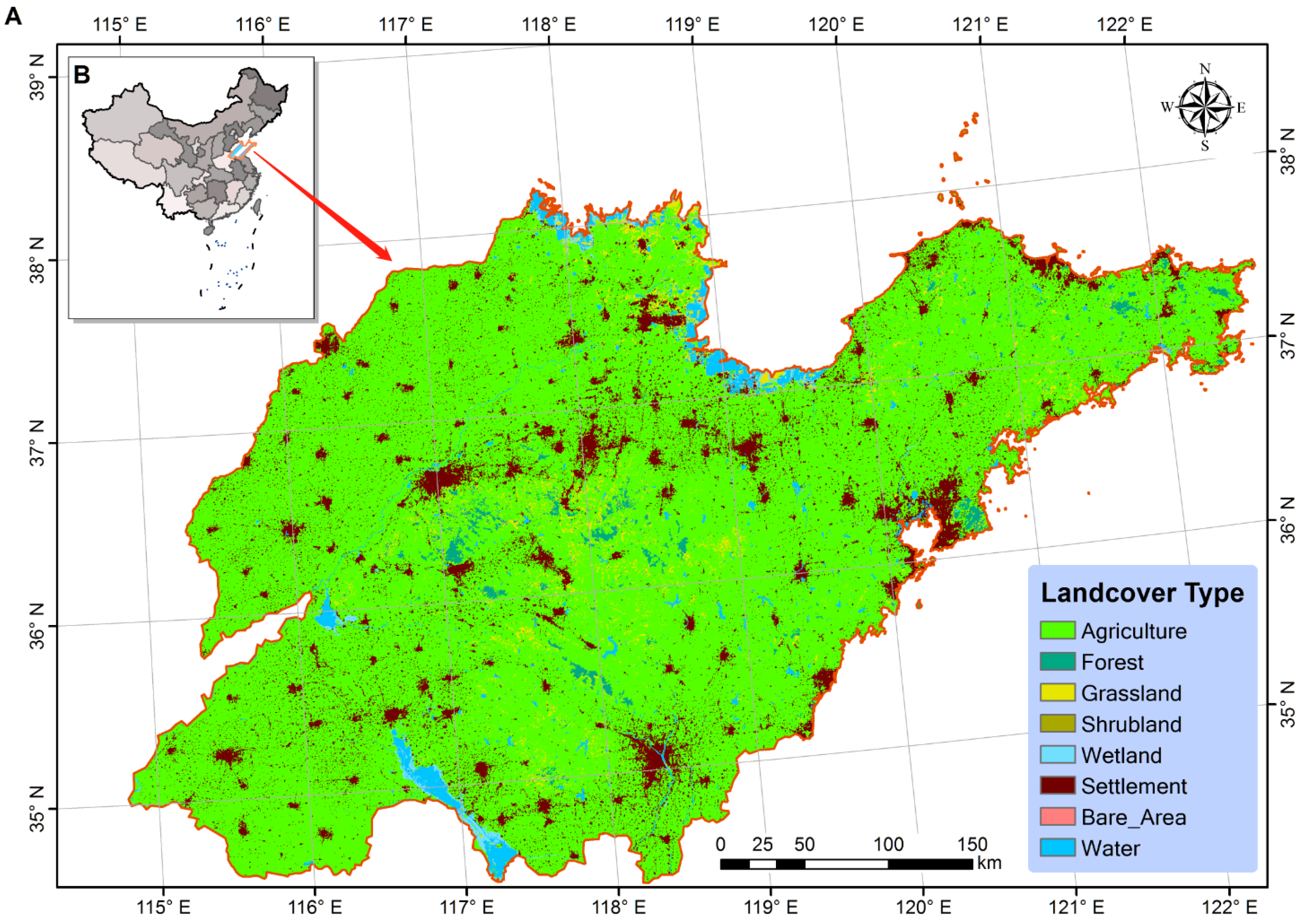
2.1. Study Area

We chose Shandong Province of China as our study area, because it has the largest amount of carbon emissions among all Chinese provinces reported in recent years and has the highest availability of corporation-level inventory data regarding carbon emissions and industrial sector attributes for use in this study (Figure 1). The gross domestic product (GDP) of Shandong Province was over USD 1 trillion (RMB ~8.31 trillion) in 2021, ranking within the top 3 provinces with the highest GDPs in China. The population of this province is over 100 million people, and the land area is 1.558 × 10⁴ km2. This province is also well known for its rapid precision farming development, especially regarding vegetable and grain cultivation. At the same time, the province represents a typical Chinese industrial structure dominated by the manufacturing industry mixed with heavy energy-intensive industries such as the power generation industry, steel industry, chemical industry, and mineral and energy extraction industry. The widely distributed farmlands within this province can provide a cool background with which IHSs can be recognized according to thermal anomaly and nightlight datasets.

2.2. Data Sources and Materials

2.2.1. VIIRS-Derived Thermal Anomaly Product

We obtained the Suomi National Polar-Orbiting Partnership (NPP) satellite-derived VIIRS active fire product representing the 2012–2020 period from the Fire Information for Resource Management System (FIRMS) data center under the administration of the National Aeronautics and Space Administration (NASA). This product can provide the global spatial distribution of thermally anomalous pixels (TAPs) at a 375 m spatial resolution, synthesized and distributed annually [14]. The dataset also provides a series of detailed thermal characteristics and attributes including the spatial locations of the observations, the brightness temperatures of the VIIRS I-4 and I-5 channels, the acquisition dates and times, the fire radiative power (FRP), and other attributive characteristics related to the confidence level and inferred fire type. In this study, we obtained a total of 0.214 million TAPs from the VIIRS active fire product (Figure 2). We retained all TAPs for the subsequent analysis considering that IHSs may be characterized by relatively low brightness temperatures and may have low confidence for active fire classification in the product.

2.2.2. ESA_CCI Land Cover Dataset

To determine the land cover type corresponding to each TAP, we used a global annual land cover time series dataset with a 300 m spatial resolution named the European Space Agency (ESA) Climate Change Initiative Land Cover (CCI-LC) product. The land cover types included in this dataset follow a classification scheme including 33 land cover types with an overall global accuracy of 71.1% [43]. We extracted the bare area and settlement categories as the mask to filter out TAPs that were related to forest fires and agricultural residual burning (see Figure 1). To effectively align these data with the temporal information characterizing the thermal anomaly time series, we obtained land cover maps from two versions of the ESA_CCI_LC product. The EAS_CCI_LC V2.0.7 product was used to cover the period from 2012 to 2015, and the EAS_CCI_LC V2.1.1 product was used for the 2016–2020 period. The annual mask area, among which the settlement class accounted for over 99.8%, tended to increase year by year from 1.28 × 10⁴ km2 in 2012 to 1.79 × 10⁴ km2 in 2020 (see Appendix A Figure A1).

2.2.3. Remotely Sensed Nighttime Light (NTL) and Gridded Population Data

It is well established that nighttime light (NTL) is a useful indicator that reflects the intensity of socioeconomic activities [44]. Thus, we assumed that NTL information, the spatiotemporal pattern of which can be quantified explicitly thanks to recent advances in satellite sensors, may be very closely linked with carbon emissions due to the fact of its strong explanatory power for many industrial-related activities such as energy consumption [45,46,47]. We used a harmonized version of the global 1 km annual NTL time series (1992–2020) product generated by Li et al. [48] to quantify the accumulated radiance of the recognized IHSs. This NTL product was sourced from the satellite sensors of the Operational Linescan System (OLS) of the Defense Meteorological Satellite Program (DMSP) and the VIIRS on the Suomi NPP. The NTL time series data representing the 1992–2013 period were derived from the intercalibrated observations of the DMSP-OLS sensor, while the 2014–2020 NTL time series data were simulated from the VIIRS observations using a harmonization process. In this study, we used the 2012–2020 NTL time series to support our analysis. We applied a nearest-neighbor interpolation approach to extract the NTL values corresponding to the recognized IHS pixels.
Population density is another ancillary datum that has frequently been used to predict carbon emissions in previous studies [49,50]. The distribution of the human footprint is assumed to be correlated with industrial energy consumption and can thus be applied to better describe carbon emissions statistically. To obtain a spatiotemporally consistent population census for the 2012–2020 period, we used a gridded world population product to estimate the human footprint intensity [51]. This product was a high-resolution (~90 m) annual global population distribution time series covering the period from 2000 to 2020. A random forest model, a type of machine learning algorithm, was combined with a collection of harmonized covariates related to factors such as topography, climate, land cover, and traffic to generate wall-to-wall population density predictions [51]. For each 90 × 90 m grid, the prediction was subsequently applied as a weighting surface and integrated with the dasymetric function to redistribute the census population counts. We then applied a spatial aggregation approach to calculate the total population count corresponding to each recognized HIS pixel in the corresponding year.

2.2.4. Reference IHS Patches

To verify the accuracy of the identified IHS objects, we randomly sampled 864 IHS polygons as a type of reference data (Figure 3). We used the high-resolution imageries embedded in Google Earth Pro software as the base maps to depict the polygon outlines according to our empirical knowledge and understanding of the local industrial sectors and their characteristics reflected in remote sensing imageries. For example, we used blast furnaces and chimneys as important targets when determining the locations of IHS objects. In addition, we also obtained the global IHS product published by Liu et al. [28] covering the period from 2012 to 2016 (denoted as Liu_2018 hereafter). The IHS objects in this product are composited in spatial polygon format (see Appendix A Figure A1). Although this product was developed using VIIRS-derived active fire time series, the polygons were organized together with no temporal information provided. We noticed that the Liu_2018 dataset omits many HIS objects in our study area, but this product was still the most reliable open-access IHS dataset available in the present case. The overall accuracy of this product is rather high (~77%) when determining subcategorical industry sectors such as cement plants and steel plants. Here, we applied these two datasets as benchmarks to validate the accuracy of the IHSs identified in our study. Because these datasets cannot be effectively aligned with the corporation-level inventory period, we did not use them in the carbon emission analysis performed in the present study.

2.2.5. Corporation-Level Inventory Data
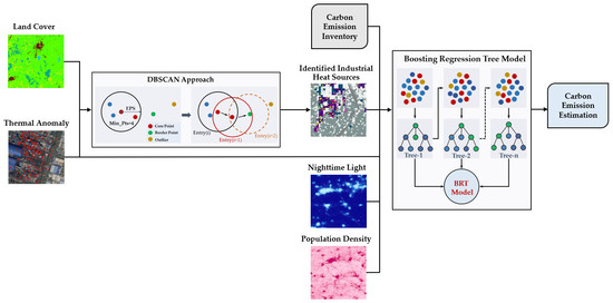
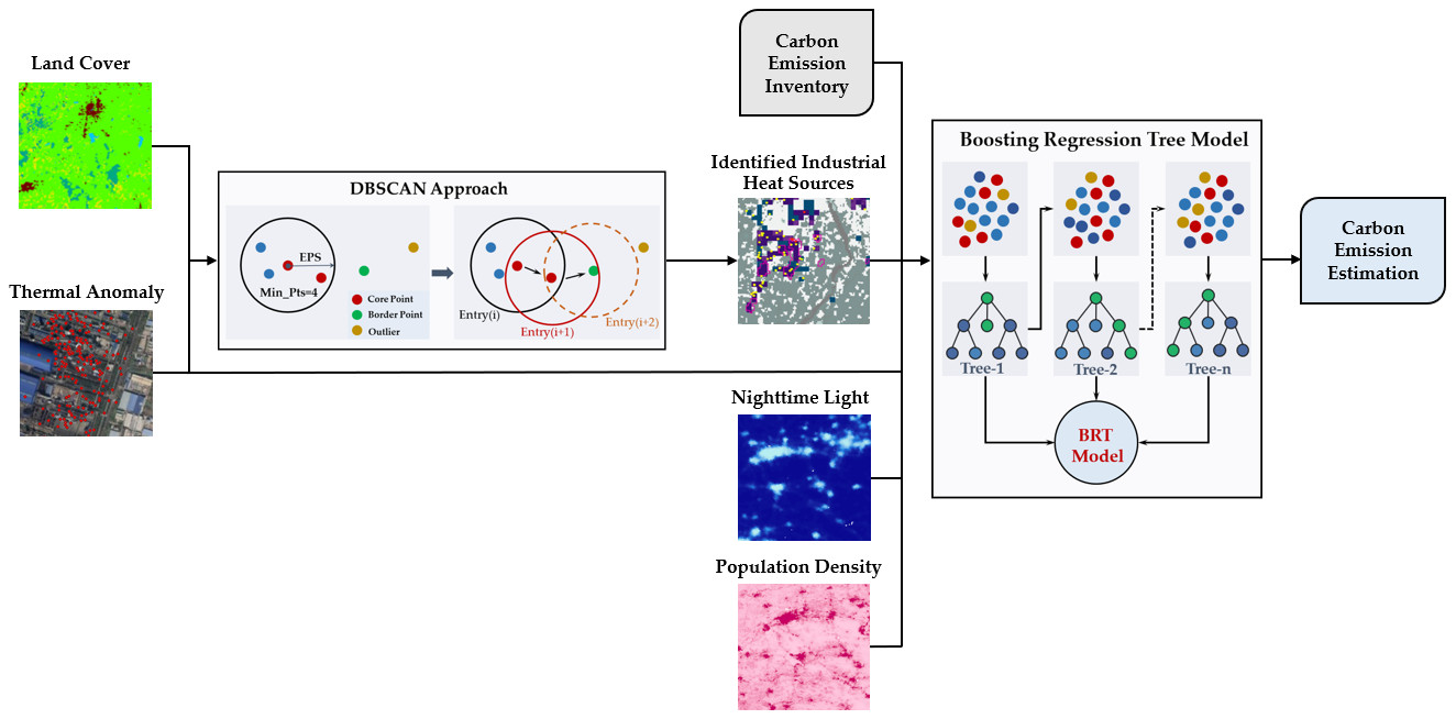
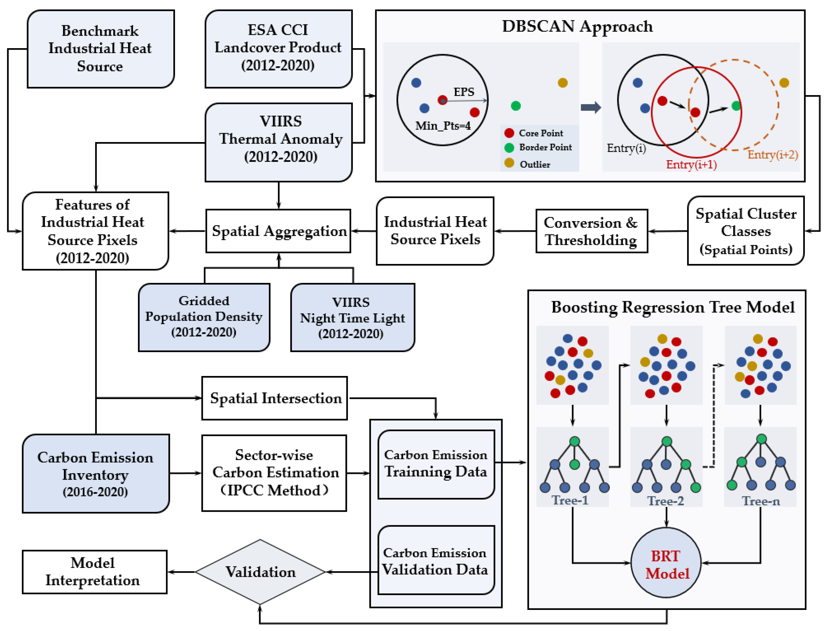
To verify the attributes of the remotely sensed IHS objects and to establish a carbon emissions estimation model, we obtained a portion of the annual corporate inventory data credited by the official authorities on environmental pollution monitoring. These data consisted of information characterizing the annual consumption of fuels (i.e., coal, coke, and natural gas) and electric power from 2016 to 2020 by each corporation that fell in the spatial extent of the identified IHS objects focused on in this study. The corporations could be classified into three main sectors according to the International Standard Industrial Classification of All Economic Activities (UNSD: 2006) including sectors related to the mining industry (denoted as Sector_B), the manufacturing industry (denoted as Sector_C), and the electricity, heat, gas, and water production and supply industry (denoted as Sector_D). These three main sectors could be further divided into 41 subcategories. Summarized descriptions of these subcategories are provided in Appendix A Table A1.
For each corporation, we calculated the carbon emission amount (in terms of CO2) following the IPCC method. The equation can be expressed as follows:
A CE = 44 12   i = 1 4 K i E i
where ACE is the amount of carbon emissions; i represents the fuel or energy type; K is the carbon emission coefficient of a given type of energy consumption; E is the amount of fuel or energy consumed. The 44/12 term is the molar ratio by which CO2 is converted to C. The conversion factor of different fuel types to standard coal equivalent and emission factors can be found in Appendix A Table A2.
For a given IHS object, we obtained the corporations that were spatially located within the object according to the corporation coordinates. We then calculated the total annual carbon emissions from these corporations and assigned the resulting value to the IHS object. We noted that the actual size of some corporations may be spatially larger than the spatial size of the corresponding IHS objects, but we could not decompose the carbon emission values to match the entire areas of these corporations due to the lack of such information; thus, we roughly assigned the total carbon emission values to the nearest IHS objects.

2.3. Workflow

We graphically summarized our workflow into two main steps (Figure 4). The first step involved identifying and characterizing the IHSs from the VIIRS thermal anomaly and auxiliary datasets by combining a spatial cluster algorithm and a series of spatial processing methods. We evaluated the accuracy of the identification results by comparing them with the reference data. Then, in the second step, we established a statistical model for estimating the carbon emissions of the identified IHSs. After the model training and validation steps, we finally interpreted the model outputs and analyzed the explanatory powers of the applied environmental variables.

2.4. Data Processing and Analysis

2.4.1. Identification of IHSs

The VIIRS thermal anomalies were observed in the form of discrete points. We reasonably assumed that these anomaly points should collocate with the core of the heat source and be spatially clustered in a small area when using long time series observations, given that industrial heat releases are stable and continuous. Such patterns can support the use of the spatial cluster analysis approach when grouping the spatially adjacent anomaly points into an object. Here, we utilized an unsupervised learning algorithm (i.e., the density-based spatial cluster applications with noise (DBSCAN) approach [52]) to distinguish whether a given point belonged to a cluster defined as the maximum set of densely connected points. This approach can be used to discover clusters of different shapes and sizes from a large amount of data containing noise and outliers.
The DBSCAN approach uses the minimum number of points (Min_Pts) and the maximum radius of the neighborhood (EPS) to justify the density reachability and density connectivity of a given point to a cluster [53]. The density reachability establishes that a point is reachable from another point if it lies within a particular distance (i.e., EPS) from the first point. Connectivity is a transitivity-based chaining approach that is used to determine whether points are located within a particular cluster. This approach randomly selects a point and estimates the reachability of all points from the selected point under the constraints imposed by the EPS and Min_Pts values. If the number of adjacent points is more than Min_Pts, the selected point is defined as a core point of a cluster; otherwise, it is labeled as a noise point, and the process moves to the next point. This process continues until all points have been classified. Because the spatial sizes of individual IHSs usually do not reach the kilometer level or the point density of annual observations, we set the Min_Pts value to four and the EPS value to 1.5 km. The DBSCAN approach is robust to noise, insensitive to the cluster shape, and has a rather high computing speed [54,55].

2.4.2. Characterization of IHSs

We used the annual VIIRS thermal anomaly product as the input data and generated a series of raw clusters that may have contained other thermal sources such as forest fires, agricultural straw burning, or fire accidents. The annual ESA_CCI_LC product was used to filter out the thermal anomaly points that fell within regions of vegetation-dominated land cover types. Due to the coarse resolution of the VIIRS data, we carried out a filtering process following the cluster analysis to prevent the potential omission of points located along edge regions. We converted the spatial points to spatial pixel objects at a 1 km resolution using the spatial overlay approach. We then characterized these pixels by spatially aggregating the corresponding thermal points and calculating the point number, mean brightness temperature, mean FRP, and duration. Some pixels contained very sparse thermal points but featured long durations due to the presence of uncertain factors such as incorrect land cover mapping or seasonal agricultural straw burning. We thus set decision rules based on the point number (>10) and duration (>30 days) to further mitigate these uncertainties. We acknowledge that such a hard classifier may remove some IHSs from the analyzed data, but it should be noted that the retained data had high confidence and should be focused on in practical applications.

2.4.3. Accuracy Assessment of IHSs

We used the two aforementioned reference IHS datasets to validate the accuracy of our results. We further processed our results to solve the issues regarding temporal and spatial inconsistencies between the datasets. To ensure that the temporal periods matched the Liu_2018 dataset, we chose our IHS results from 2012 to 2016 and generated a mosaic to improve the temporal consistency between the two datasets. For the sample data, we generated a full 2012–2020 composite of our IHS results to promote temporal consistency between the two datasets. Because the two reference datasets both represented partial samples compared to the true IHS information, we did not think they could be used to fully evaluate the accuracies of the IHS results in terms of the commission and omission errors. Therefore, we used two measures to evaluate the accuracy of our identifications. At the patch level, we calculated the rate of the overlapping area (ROA) for each referenced IHS object, obtained the basic relevant statistics, such as the mean values and standard deviations, and constructed a histogram to evaluate the patch-level accuracy. For the whole dataset, we calculated the percentage of referenced IHSs that overlapped with our identified results.
To determine the industrial sectors corresponding to the identified IHS objects, we did not assign categories or subcategories to the IHS objects as has been conducted previously. As we noticed that one remotely sensed IHS object can cover multiple corporations that belong to different industrial sectors, we used all corporations covered by each IHS and obtained statistics related to the corporation abundances from 2016 to 2020. We subsequently analyzed the composition of the validated IHSs to address our first objective.

2.5. Estimation of Industrial Carbon Emissions

To ensure consistency with the IHS analysis, we also converted the corporate carbon emissions inventory into a raster dataset at a 1 km resolution. We followed the bottom-up approach to generate a carbon emission raster in which the carbon emissions of a given pixel were assigned using the sum of all corporations within the corresponding area. The overlapping pixels between the remotely sensed IHSs and carbon emission grids were then extracted and utilized as the training data in the subsequent modeling work. The summary statistics and descriptions of explanatory variables for the carbon emission modeling can be seen in Table 1.

2.5.1. BRT Modeling

Since the remotely sensed features can only provide parameters that are related to carbon emissions, the carbon emission estimation via remote sensing is overwhelmingly empirical. Here, we applied the BRT algorithm to establish the empirical relationships. We did not choose deep learning algorithms, because their “black box” nature would limit us to interpreting those empirical relationships and could be supported in the BRT algorithm. The BRT model is a tree-based ensemble learning algorithm proposed by Elith et al. [56]. This algorithm is robust for processing nonlinear relationships between explanatory and response variables. In the model, the boosting algorithm is integrated with the decision tree model to enhance the predictive ability of the model by combining weak models into a relatively strong model. The boosting algorithm can help the BRT model create weighted trees to improve the subsequently constructed trees, meaning that the model takes into account the error in the prediction of the previous tree when fitting the next tree. By using this sequential procedure, the accuracy of the model results is continuously improved. In addition, the model has a relatively strong tolerance to unbalanced data with skewness, missing values, and complex interactions among predictors. It is widely reported that the BRT model has a stronger regression power than most other machine learning algorithms, such as the well-known random forest model and the support vector machine algorithm, in the same application scenarios.
The BRT model has two important parameters that must be defined by the user: the so-called tree complexity and the learning rate. The tree complexity controls the number of branches in each tree, and the learning rate determines the contribution of each tree to the growing model. Together, these parameters determine the number of trees required to obtain the optimal prediction. We followed the parameter setting recommendations proposed by Elith, Leathwick, and Hastie [56], setting the tree complexity to 3 and the learning rate to 0.01 to allow the model to grow a sufficient number of trees. We used the relative importance as an indicator to quantify the contribution of predictors aiming to improve the model explanatory strength to the variance in carbon emissions.

2.5.2. Accuracy Assessment

The BRT model’s performance was evaluated by comparing the model-fitted data with the gridded corporate inventory data. We calculated the variance explained (R2) and the index of agreement (IOA) to evaluate the goodness of fit of the model results. In addition, we also calculated the root mean squared error (RMSE) and the mean absolute percentage error (MAPE) as criteria to assess the errors in the results. These metrics can be calculated using the following equations:
  R 2 = [ i = 1 N ( Y o , i Y ¯ o ) ( Y m , i Y ¯ m ) i = 1 N ( Y o , i Y ¯ o ) 2 i = 1 N ( Y m , i Y ¯ m ) 2 ] 2
    I O A = 1 i = 1 N ( Y o , i Y m , i ) 2 i = 1 N ( | Y o , i Y ¯ o | + | Y m , i Y ¯ o | ) 2
R M S E = 1 N i = 1 N ( Y o , i Y m , i ) 2  
M A E = 1 N i = 1 N | Y o , i Y m , i |
where   Y o is the observation value and Y m is the predicted value; Y ¯ o is the average observation values and Y ¯ m is the average predicted value; N is the number of observation data.

3. Results

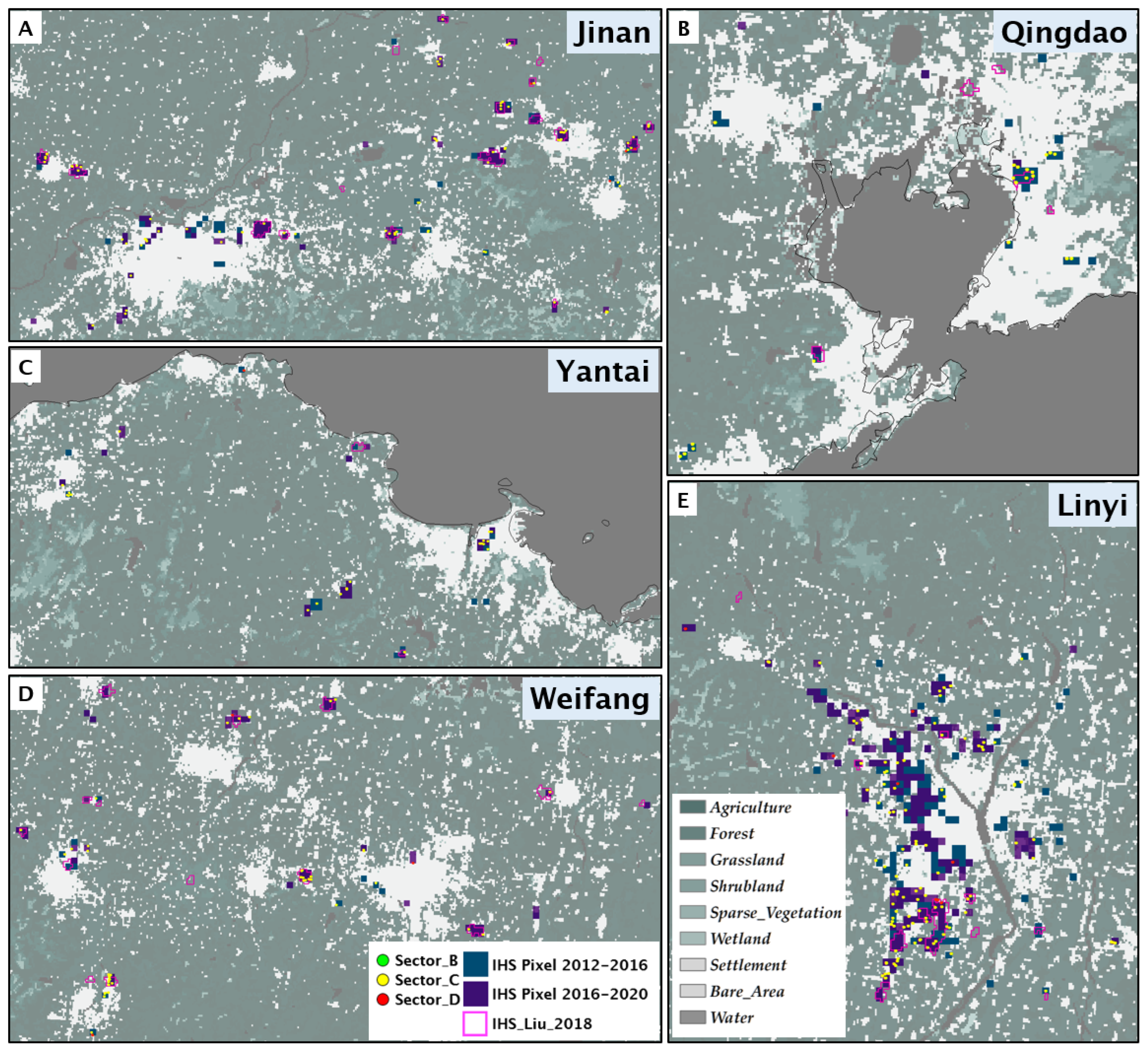
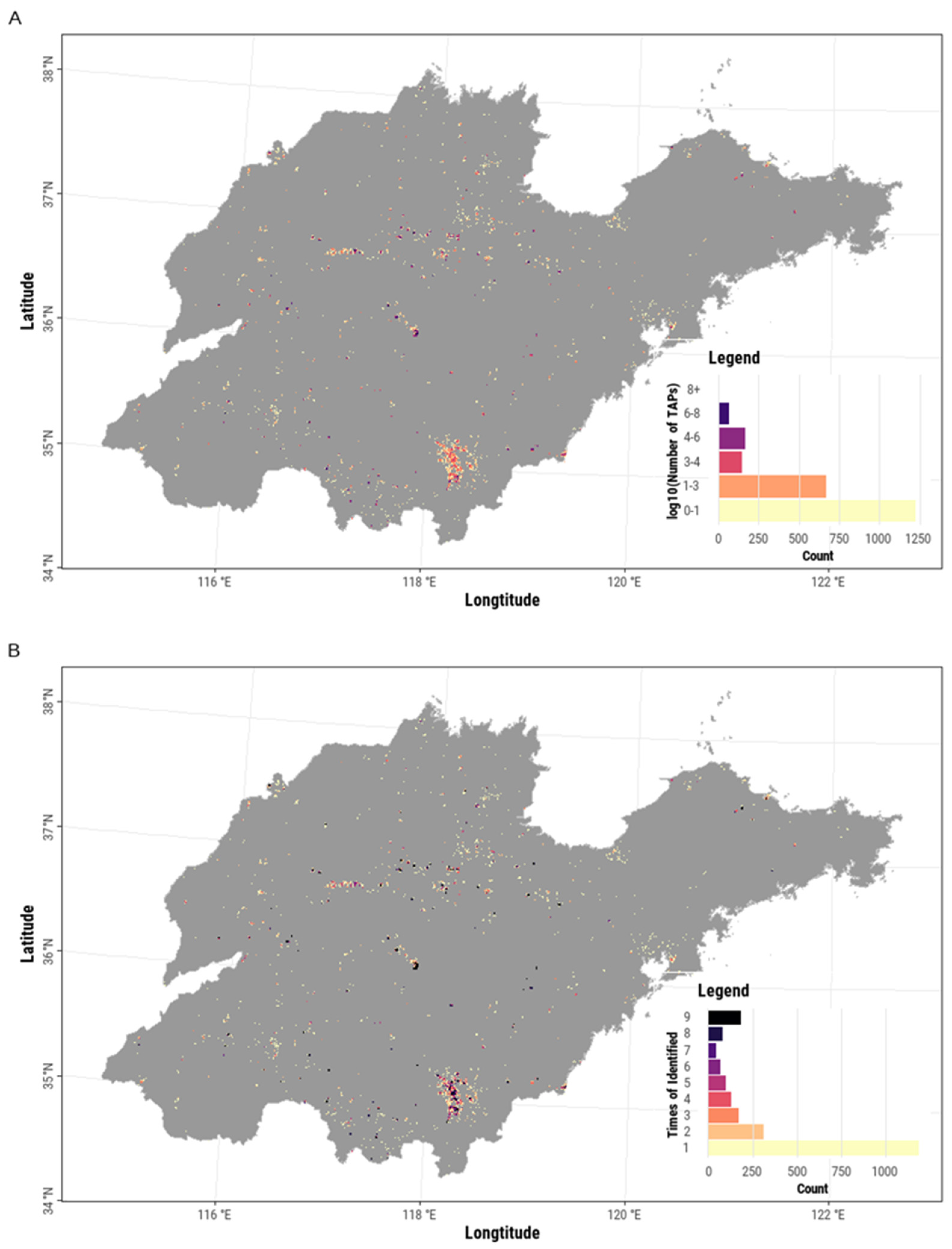
3.1. Identification of IHSs

We identified a total of 4031 IHS pixels (1 × 1 km) containing approximately 0.101 million TAPs identified from 2012 to 2020 (Table 2). The annual number of IHS pixels was significantly correlated with the corresponding number of raw TAPs (r = 0.64, p < 0.02). As a result of government control on agricultural straw burning, the raw TAPs showed a remarkable decreasing trend. However, we found that the retained TAPs used to identify IHSs did not represent a statistically significant trend. In contrast, the fraction of retained TAPs exhibited a significantly increasing trend as the number of raw TAPs decreased (r = −0.88, p < 0.02), suggesting that the control of agricultural straw burning helped reduce the uncertainties associated with thermal anomalies.
The DBSCAN clusters, from which the IHS pixels were obtained, also decreased along with the dynamics of the annual raw TAPs (r = 0.98, p < 0.02), ultimately causing a reduction in the number of raw IHS pixels. This procedure excluded approximately 52% of the raw TAPs and generated an average of 541 clusters each year. The further thresholding procedure filtered approximately 42% of the raw IHS pixels, comprising pixels that could not meet the decision rules. We generated accumulated TAPs for each IHS pixel and found that over 20% contained more than 1000 points between 2012 and 2020 (Figure 5A). The IHS pixels were sparsely distributed in general but exhibited a clustered pattern in the south and central parts of the province. Approximately 30% of the IHS pixels were identified more than three times, and approximately 9.4% of the total number of IHS pixels were identified every year (Figure 5B).

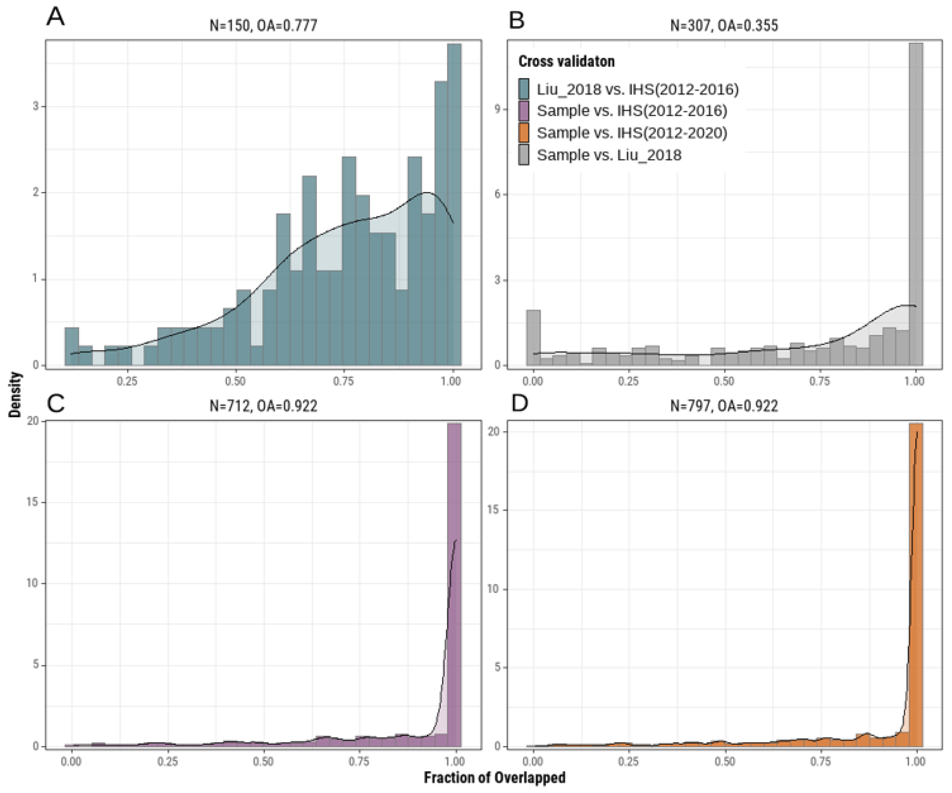
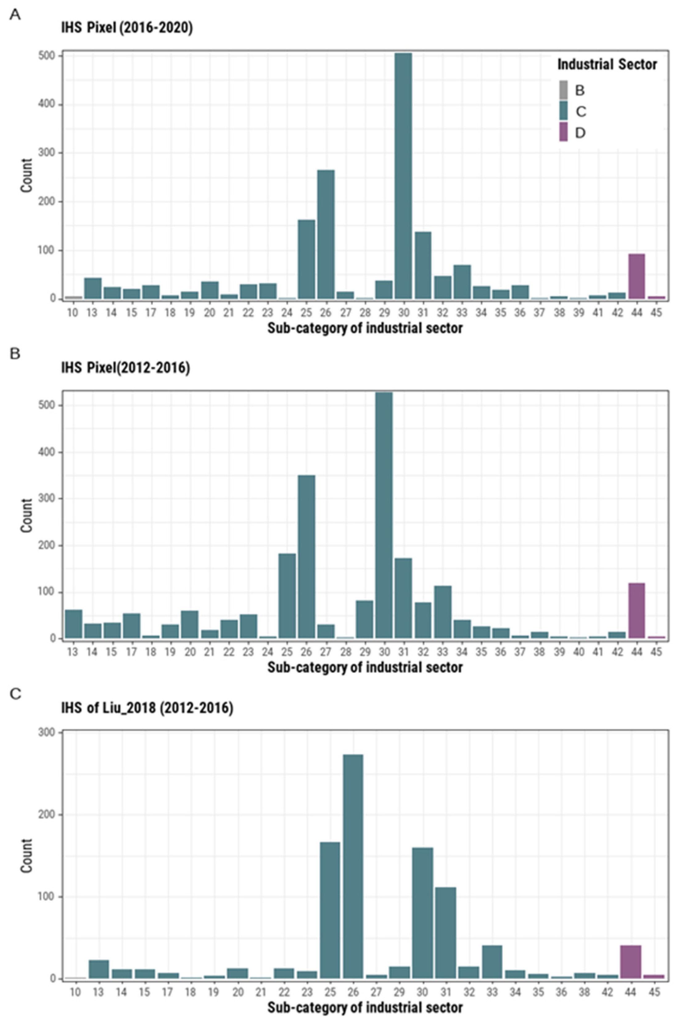
3.2. Comparison with the Referenced IHSs

Regarding the relatively coarse resolution of our analysis, the IHS pixel boundaries did not strictly align with the spatial extent of each industrial corporation; however, we still found that the IHS pixels could cover most areas corresponding to these corporations, especially the locations from which heat was released (see Appendix A Figure A2). To obtain an unbiased accuracy estimation, we compared our results with two types of benchmark IHS datasets. We used only the IHS pixels corresponding to the 2012–2016 period for the comparison with the Liu_2018 data but used all IHS pixels for the comparison with the sample data to guarantee that the comparisons were carried out on consistent time scales. Any duplicate IHS pixels that were identified multiple times were removed before the comparisons.
We found that 150 out of 193 patches (OA = 77.7%) from the Liu_2018 data (Figure 6A) and 797 out of 864 patches (OA = 92.2%) from the sample data (Figure 6D) overlapped with our IHS pixels. We also compared the two reference datasets as a further reference, although they represented different periods. We identified 307 patches (OA = 35.5%) from the sample data that overlapped with the Liu_2018 data (Figure 6B), while as a comparison, the IHS pixels of 2012–2016 (OA = 82.4%) overlapped with 712 patches (Figure 6C). We applied an ROA ≥ 0.75 as a criterion to evaluate the state of IHS overlap. The results showed that 84.8% of overlapped patches (with 2012–2020 IHS pixels, Figure 6D) from the sample data and 58% of overlapped patches (with 2012–2016 IHS pixels, Figure 6A) from Liu_2018 met the standard. Approximately 83.1% overlapped patches (with 2012–2016 IHS pixels, Figure 6C) and 61.3% overlapped patches (with Liu_2018, Figure 6B) from the sample data met the standard.

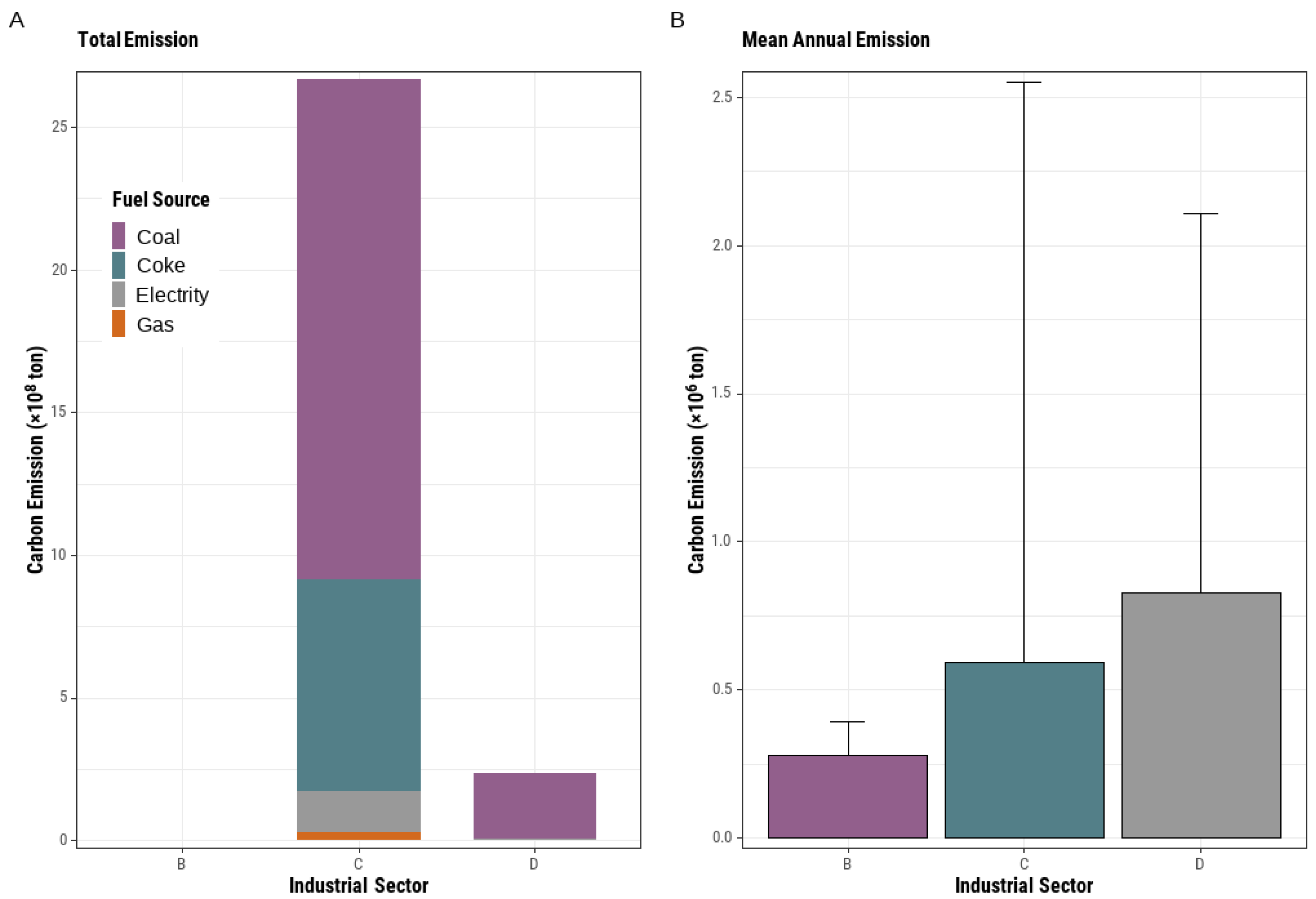
3.3. Comparison with Corporate Inventory Data

According to the spatial extents of the remotely sensed IHS pixels (2012–2020), we obtained a total of 5443 corporations with explicit attributes corresponding to the industrial sectors and energy consumption amounts (Table 3). Integrating IHS pixels from multiple years can increase the coverage area and thereby increase the number of cross-validated corporations. We found that the IHS pixels contained similar manufacturing industry (i.e., Sector_C) and energy-related industry (i.e., Sector_D) percentages, suggesting very similar capacities of the thermal anomalies for detecting IHS objects from these two domains. Because the manufacturing industry (i.e., Sector_C) occupied approximately 95.0% of the total number of analyzed corporations, it is reasonable that most of the identified corporations belonged to Sector_C.
As shown in Figure 7, the manufacturing of nonmetallic mineral products (e.g., cement, glass, graphite, and carbon products) and the chemical industry were the top two subcategories among the identified Sector_C corporations, followed by the smelting and pressing of ferrous metals (e.g., steel produce), fuel-processing industries (e.g., petroleum and coal), and the manufacturing of metal products. Electric heat production (i.e., thermal power plants) was the primary subcategory representing Sector_D.

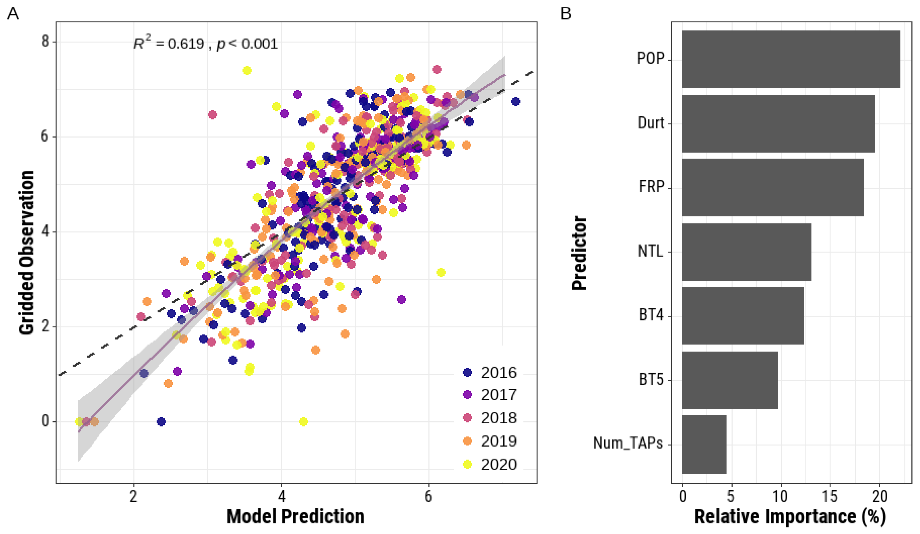
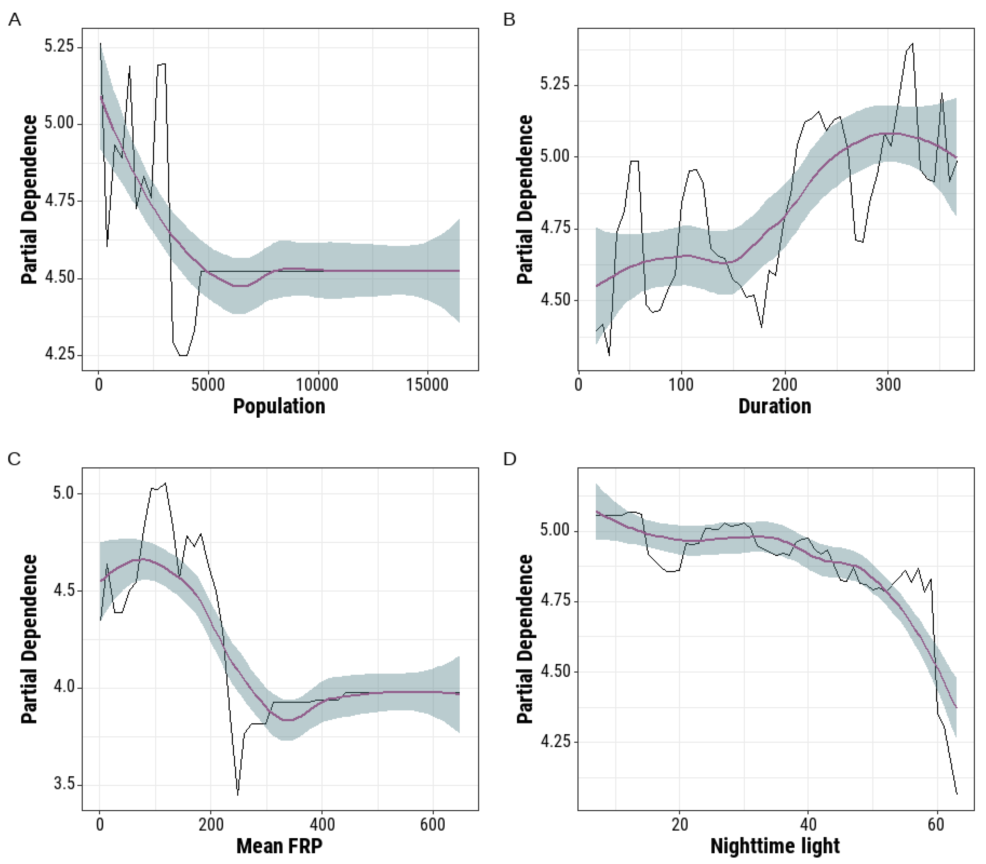
3.4. BRT Modeling Performance Evaluation

We used 661 IHS pixels that overlapped with the gridded carbon emission dataset characterizing the 2016–2020 period to establish the regression model. The results showed that the BRT model performed reasonably well, as approximately 61.9% of the variance was explained, and the IOA was 0.83, indicating a high goodness of fit between the model predictions and corporate inventory data (Figure 8A). Across the five years, the model accuracy in terms of the MAPE was 0.16, while the RMSE was 0.92. Figure 8B shows the relative importance rankings of all explanatory variables. As the figure shows, the population density (22.2%) and two thermal anomaly related features, namely, the duration (19.5%) and the FRP (19.6%), as well as the nighttime light (13.2%), had larger contributions to the predictive power of the BRT model than the other three analyzed variables.

4. Discussion

In this study, we evaluated the capacity of remotely sensed thermal anomaly products to identify IHSs. Based on the DBSCAN approach and a land cover dataset, we generated the wall-to-wall IHS distribution in Shandong Province and generally found that the modeled IHS results were well aligned with the IHSs in the two independent reference datasets and were confirmed by high-resolution satellite imagery. These IHS pixels were mostly located in the outskirts of cities (Figure 9), but some were spatially continuous within cities dominated by manufacturing (e.g., Linyi city, Figure 9E). Isolated IHS objects were generally easy to detect due to the relatively cool background conditions and clustered thermal anomaly patterns. In most cities, the IHS objects located in downtown areas were rarely represented in the reference data but were well captured in our analysis. We considered that this may have been because our analysis was conducted at a larger grain size than the reference data, which will increase the opportunity to retain more fire spots in the identification.
We also considered some factors that may have influenced the consistency between our results and the reference datasets. First, because we filtered out thermal points located in farmlands and forests according to the ESA_CCI land cover product, some IHS patches in the Liu_2018 product located in farmlands and forests were not identified in our study. Second, the accuracy of our IHS identification results was partially limited by the quality of the land cover mapping, but such a filtering process was useful for reducing the confusion and uncertainty that arise from biomass burning during wildfires or anthropogenic fires. Since the DBSCAN approach was physically based and the raw data (i.e., fire spots and landcover maps) could be obtained easily for other regions, our methods can be expanded directly to other regions. In addition, in contrast to some other studies in which combined datasets covering multiple years of observation were used [23,25,28], our approach to mapping IHS annually was straightforward. This method can be beneficial in aiding policymakers who track the temporal dynamics of IHS abundance, but we admit that the consequently shorter period decreases the accumulation of thermal points around any given IHS and increases the potential for omission errors.
Through a comparison with corporate-level inventory data, our results clearly showed that the identified IHS pixels mostly belonged to the EIIS, especially to the heavy industries mainly belonging to the chemical industry and the manufacturing of nonmetallic mineral products such as the cement, glass, graphite, and carbon production industries. Corporations of Sector_C accounted for most of the total carbon emissions due to the large number of individual corporations in this sector, but the individual corporations of Sector_D had remarkably higher mean annual emission amounts than other industrial sectors (Figure 10A). From the perspective of fuel sources, coal and coke consumption contributed the majority of the carbon emissions associated with the identified IHSs (Figure 10B). The EIIS corporations that use coal and coke as fuel resources usually emit considerable waste heat into the environment during their processing operations [57], while corporations that rely primarily on electricity to support their operations may generate little heat waste, and facilities such as constructions or shelters can also shield industrial heat emissions. Although our results can cover these corporation components, we believe that the spatial points identified on behalf of the spatial locations of these corporations fell in the IHS pixels by chance or were not specifically identified as members of the EIIS. Thus, we concluded that the identified IHS pixels could capture the EIIS corporations that contributed to the majority of the carbon emissions.
The BRT model explained a considerable amount of variance in the total carbon emissions estimated using the bottom-up inventory approach, suggesting that it is feasible to estimate carbon emissions by combining machine learning approaches with environmental variables that are linked with carbon emissions. We selected explanatory variables that were sensitive to social economics and human activity footprints for model training. The training data predictors were obtained from global gridded products that were carefully investigated and produced with broad public credibility and are well accepted by the academic community. Benefiting from the strong ability of the BRT model to handle complex and nonlinear relationships between predictors and response variables (Figure 11), we found that the population density, FRP, and NTL showed negative relationships and notable nonmonotonicity with carbon emissions, while the tendency curve between duration and carbon emissions showed a positive relationship.
For the population density, we generally observed a decreasing carbon emissions trend as the population number increased (Figure 11A). This result was consistent with the general reality that high-emission industries are usually located in urban periphery regions, where the population density is not as high as that in downtown areas where low-emissions corporations are usually distributed. Regarding the duration, we found that IHS objects with relatively long thermal anomaly durations led to increased carbon emissions; however, we also noted that this relationship curve fluctuated considerably (Figure 11B). We believe the underlying reason for this fluctuation was that multiple corporations are often located within a given IHS pixel, and the operating temperature of corporations belonging to different industrial sectors may differ substantially in their processing periods [58]. These discrepancies may introduce uncertainties, as we could not attribute the identified thermal anomalies to specific corporations. The mean FRP, a measure of thermal emissivity, and the observed thermal anomaly duration were found to be important variables that could improve the fit of the carbon emissions (Figure 11C). These two thermal-related variables represented rather complex response curves. Ignoring the rugged curve regions with large uncertainties, we generally found that carbon emissions increased sharply as the FRP increased but easily reached a saturation situation. For NTL, we found that areas of high brightness corresponded to low carbon emissions (Figure 11D). The underlying reason for this is similar to that of population density; high-emission industries are usually located in urban periphery regions, where the NTL is not as high as that in downtown areas. Moreover, regions without any nighttime lights do not mean the regions have no CO2 emissions [59]. For example, some EIIS corporations only operate during the daytime but stop operating and turn off all lights at night.
Although the modeling framework was straightforward and the outputs were validated, we noted that the estimation approach could be further improved in future studies. First, based on corporate inventory, we learned that the mean carbon emission amount was considerably differentiated among industrial sectors. We believe that the model performance could be improved by involving the attribute information of the identified IHS objects. Such information can perhaps be obtained from the POI services provided by web platforms or databases such as Google Maps, Baidu Maps, and OpenStreetMap. Ideally, these databases could be promoted to form a more comprehensive characterization of IHS objects; however, it should also be noted that mismatch and omission issues may reduce their usage. Second, we estimated only the carbon emissions associated with the identified IHS objects, which may account for only a part of the overall carbon emissions. Future studies should focus on improving this omission problem during IHS identification, especially when identifying IHSs containing EIIS corporations. Simultaneously, to ensure spatial consistency with the explanatory variables, we identified IHSs at a relatively coarse spatial resolution. This resolution could be further improved by applying high-resolution satellite imageries, especially nighttime thermal infrared imageries. In addition, though the BRT model is simple and novel, we noted that the model fitting can be further improved by using deep learning approaches regarding their high performance in handling classification and regression problems. However, caution is required due to the fact of their disadvantages such as greater computational burden, proneness to overfitting, and the empirical nature of model development.

5. Conclusions

In summary, in this study, we described a thermal anomaly based approach to identifying IHS objects and modeling their carbon emissions using machine learning. Based on the DBSCAN algorithm, we identified approximately 414 IHS pixels (1 × 1 km) per year in Shandong Province from 2012 to 2020. The cross-validation showed that our results were consistent with the reference datasets. According to the corporation-level inventory dataset, we highlighted that the remotely sensed thermal anomalies were sensitive to the IHSs originating from EIIS-related corporations, especially thermal power plants, cement plants, the chemical industry, the steel production industry, and other nonmetallic mineral production industries (e.g., glass, graphite, and carbon production). We followed the bottom-up method to calculate the corporation-level carbon emissions and upscaled them to match the IHS pixels. Based on the BRT model, we found that the population density, NTL, and remotely sensed thermal features were useful for improving the model fitting of the carbon emissions in the identified IHS pixels. In this study, we proposed a novel and straightforward framework that can provide valuable support for understanding the spatiotemporal dynamics of IHSs, especially those related to the EIIS. We also provided an alternative approach for estimating industrial carbon emissions, and although this approach can account for only a limited fraction of the total emission amount, it can help monitor industrial activities in the shift toward a cleaner and lower-carbon environment. Future works need to improve the identification of IHS objects with low thermal emissivity to reduce the omission problems and involve multiple-source datasets at finer scales to characterize IHS object more comprehensively and accurately.

Author Contributions

Conceptualization, X.K., X.W. and M.J.; methodology, X.K.; software, X.K.; validation, X.W.; formal analysis, X.K.; data curation, X.W. and M.J.; writing—original draft preparation, X.K.; writing—review and editing, X.K., X.W., M.J. and Q.L.; visualization, M.J.; supervision, Q.L. All authors have read and agreed to the published version of the manuscript.

Funding

This research received no external funding.

Data Availability Statement

Not applicable.

Conflicts of Interest

The authors declare no conflict of interest.

Appendix A

Table A1. A brief description of the subcategorical industrial sectors of mining, manufacturing, and energy industries that have the potential to be detected as industrial heat sources via thermal remote sensing.
CodeIndustry Sector
BMining
06Mining and Washing of Coal Industry
07Extraction of Petroleum and Natural Gas
08Ferrous Metal Mining and Selection Industry
09Nonferrous Metal Mining and Selection Industry
10Nonmetallic Mining and Selection Industry
11Mining Professional and Auxiliary Activities
12Other Mining Industry
CManufacturing
13Processing of Food from Agricultural Products
14Manufacture of Foods
15Manufacture of Beverages
16Manufacture of Tobacco
17Manufacture of Textile
18Manufacture of Textile Wearing Apparel, Footwear, and Caps
19Manufacture of Leather, Fur, Feather, and Related Products
20Processing of Timber, Manufacture of Wood, Bamboo, Rattan, Palm, and Straw Products
21Manufacture of Furniture
22Manufacture of Paper and Paper Products
23Printing, Reproduction of Recording Media
24Manufacture of Articles for Culture, Education, and Sport Activities
25Processing of Petroleum, Coking, Processing of Nuclear Fuel
26Manufacture of Raw Chemical Materials and Chemical Products
27Manufacture of Medicines
28Manufacture of Chemical Fibers
29Manufacture of Rubber and Plastics
30Manufacture of Nonmetallic Mineral Products
31Smelting and Pressing of Ferrous Metals
32Smelting and Pressing of Nonferrous Metals
33Manufacture of Metal Products
34Manufacture of General Purpose Machinery
35Manufacture of Special Purpose Machinery
36Manufacture of Automobile
37Manufacture of Railways, Shipbuilding, Aerospace, and Other Transportation Equipment
38Manufacture of Electrical Machinery and Equipment
39Manufacture of Communication Equipment, Computers, and Other Electronic Equipment
40Manufacture of Measuring Instruments and Machinery for Cultural Activity and Office Work
41Manufacture of Artwork and Other Manufacturing
42Recycling and Disposal of Waste
43Repair and Installation of Machinery and Equipment
DProduction and Supply of Electricity, Gas, and Water
44Production and Supply of Electric Power and Heat Power
45Production and Supply of Gas
46Production and Supply of Tap Water
Table A2. Conversion factor of power generation coal to standard coal equivalent (SCE) and CO2 emission factor for different fuel types.
Energy TypeConversion Factor to SCE
(Unit: tSCE/t)
Carbon Emission Factor
(×104 tC/104 tSCE)
CFSCECEF
Raw Coal0.71430.7559
Coke0.97140.855
Natural Gas *1.330.4483
Electricity *-0.272
* The unit of natural gas conversion to CO2 emissions is t/103 m3, and the unit of electricity conversion to CO2 emissions is t C/103 kWh.
Figure A1. The annual variation in the total masked area (i.e., settlement and bare area) between 2012 and 2020.
Remotesensing 14 02901 g0a1
Figure A2. Examples of comparison between the industrial heat source (IHS) pixels of this study and two reference data (i.e., the sample data and Liu_2018 data). The dots represent the corporations falling in IHS pixels.
Remotesensing 14 02901 g0a2

References

  1. Guo, J.; Su, T.; Chen, D.; Wang, J.; Li, Z.; Lv, Y.; Guo, X.; Liu, H.; Cribb, M.; Zhai, P. Declining Summertime Local-Scale Precipitation Frequency Over China and the United States, 1981–2012: The Disparate Roles of Aerosols. Geophys. Res. Lett. 2019, 46, 13281–13289. [Google Scholar] [CrossRef] [Green Version]
  2. Hoegh-Guldberg, O.; Jacob, D.; Taylor, M.; Bolanos, T.G.; Bindi, M.; Brown, S.; Camilloni, I.A.; Diedhiou, A.; Djalante, R.; Ebi, K.; et al. The human imperative of stabilizing global climate change at 1.5 degrees C. Science 2019, 365, 1263. [Google Scholar] [CrossRef] [PubMed] [Green Version]
  3. Burke, S.E.L.; Sanson, A.V.; Van Hoorn, J. The Psychological Effects of Climate Change on Children. Curr. Psychiatry Rep. 2018, 20, 1–8. [Google Scholar] [CrossRef] [PubMed]
  4. Sintayehu, D.W. Impact of climate change on biodiversity and associated key ecosystem services in Africa: A systematic review. Ecosyst. Health Sustain. 2018, 4, 225–239. [Google Scholar] [CrossRef] [Green Version]
  5. Mengel, M.; Nauels, A.; Rogelj, J.; Schleussner, C.F. Committed sea-level rise under the Paris Agreement and the legacy of delayed mitigation action. Nat. Commun. 2018, 9, 601. [Google Scholar] [CrossRef] [Green Version]
  6. Rosen, M.A. Energy Sustainability with a Focus on Environmental Perspectives. Earth Syst. Environ. 2021, 5, 217–230. [Google Scholar] [CrossRef]
  7. IPCC. Climate Change 2022: Mitigation of Climate Change. Contribution of Working Group III to the Sixth Assessment Report of the Intergovernmental Panel on Climate Change; IPCC: Cambridge, UK; New York, NY, USA, 2022. [Google Scholar]
  8. Shan, Y.L.; Guan, D.B.; Zheng, H.R.; Ou, J.M.; Li, Y.; Meng, J.; Mi, Z.F.; Liu, Z.; Zhang, Q. Data Descriptor: China CO2 emission accounts 1997–2015. Sci. Data 2018, 5, 170201. [Google Scholar] [CrossRef] [Green Version]
  9. Wang, S.; Zhang, Y.; Hakkarainen, J.; Ju, W.; Liu, Y.; Jiang, F.; He, W. Distinguishing Anthropogenic CO2 Emissions From Different Energy Intensive Industrial Sources Using OCO-2 Observations: A Case Study in Northern China. J. Geophys. Res.-Atmos. 2018, 123, 9462–9473. [Google Scholar] [CrossRef]
  10. Liu, F.; Zhang, Q.; Tong, D.; Zheng, B.; Li, M.; Huo, H.; He, K. High-resolution inventory of technologies, activities, and emissions of coal-fired power plants in China from 1990 to 2010. Atmos. Chem. Phys. 2015, 15, 13299–13317. [Google Scholar] [CrossRef] [Green Version]
  11. Sekertekin, A.; Arslan, N. Monitoring thermal anomaly and radiative heat flux using thermal infrared satellite imagery-A case study at Tuzla geothermal region. Geothermics 2019, 78, 243–254. [Google Scholar] [CrossRef]
  12. Elvidge, C.D.; Baugh, K.; Zhizhin, M.; Hsu, F.C.; Ghosh, T. VIIRS night-time lights. Int. J. Remote Sens. 2017, 38, 5860–5879. [Google Scholar] [CrossRef]
  13. Giglio, L.; Csiszar, I.; Restás, Á.; Morisette, J.T.; Schroeder, W.; Morton, D.; Justice, C.O. Active fire detection and characterization with the advanced spaceborne thermal emission and reflection radiometer (ASTER). Remote Sens. Environ. 2008, 112, 3055–3063. [Google Scholar] [CrossRef]
  14. Schroeder, W.; Oliva, P.; Giglio, L.; Csiszar, I.A. The New VIIRS 375 m active fire detection data product: Algorithm description and initial assessment. Remote Sens. Environ. 2014, 143, 85–96. [Google Scholar] [CrossRef]
  15. Schroeder, W.; Oliva, P.; Giglio, L.; Quayle, B.; Lorenz, E.; Morelli, F. Active fire detection using Landsat-8/OLI data. Remote Sens. Environ. 2016, 185, 210–220. [Google Scholar] [CrossRef] [Green Version]
  16. Chuvieco, E.; Lizundia-Loiola, J.; Lucrecia Pettinari, M.; Ramo, R.; Padilla, M.; Tansey, K.; Mouillot, F.; Laurent, P.; Storm, T.; Heil, A.; et al. Generation and analysis of a new global burned area product based on MODIS 250 m reflectance bands and thermal anomalies. Earth Syst. Sci. Data 2018, 10, 2015–2031. [Google Scholar] [CrossRef] [Green Version]
  17. Earl, N.; Simmonds, I. Spatial and Temporal Variability and Trends in 2001-2016 Global Fire Activity. J. Geophys. Res.-Atmos. 2018, 123, 2524–2536. [Google Scholar] [CrossRef]
  18. Li, H.; Zhou, Y.; Li, X.; Meng, L.; Wang, X.; Wu, S.; Sodoudi, S. A new method to quantify surface urban heat island intensity. Sci. Total Environ. 2018, 624, 262–272. [Google Scholar] [CrossRef]
  19. Meng, Q.; Zhang, L.; Sun, Z.; Meng, F.; Wang, L.; Sun, Y. Characterizing spatial and temporal trends of surface urban heat island effect in an urban main built-up area: A 12-year case study in Beijing, China. Remote Sens. Environ. 2018, 204, 826–837. [Google Scholar] [CrossRef]
  20. Ahmed, S. Assessment of urban heat islands and impact of climate change on socioeconomic over Suez Governorate using remote sensing and GIS techniques. Egypt. J. Remote Sens. Space Sci. 2018, 21, 15–25. [Google Scholar] [CrossRef]
  21. Wang, W.M.; Liu, K.; Tang, R.; Wang, S.D. Remote sensing image-based analysis of the urban heat island effect in Shenzhen, China. Phys. Chem. Earth 2019, 110, 168–175. [Google Scholar] [CrossRef]
  22. Pan, Z.K.; Wang, G.X.; Hu, Y.M.; Cao, B. Characterizing urban redevelopment process by quantifying thermal dynamic and landscape analysis. Habitat Int. 2019, 86, 61–70. [Google Scholar] [CrossRef]
  23. Ma, C.H.; Yang, J.; Chen, F.; Ma, Y.; Liu, J.B.; Li, X.P.; Duan, J.B.; Guo, R. Assessing Heavy Industrial Heat Source Distribution in China Using Real-Time VIIRS Active Fire/Hotspot Data. Sustainability 2018, 10, 4419. [Google Scholar] [CrossRef] [Green Version]
  24. Ma, Y.; Ma, C.H.; Liu, P.; Yang, J.; Wang, Y.Z.; Zhu, Y.Q.; Du, X.P. Spatial-Temporal Distribution Analysis of Industrial Heat Sources in the US with Geocoded, Tree-Based, Large-Scale Clustering. Remote Sens. 2020, 12, 3069. [Google Scholar] [CrossRef]
  25. Ma, C.; Niu, Z.; Ma, Y.; Chen, F.; Yang, J.; Liu, J. Assessing the Distribution of Heavy Industrial Heat Sources in India between 2012 and 2018. Isprs Int. J. Geo-Inf. 2019, 8, 568. [Google Scholar] [CrossRef] [Green Version]
  26. Xia, H.P.; Chen, Y.H.; Quan, J.L. A simple method based on the thermal anomaly index to detect industrial heat sources. Int. J. Appl. Earth Obs. Geoinf. 2018, 73, 627–637. [Google Scholar] [CrossRef]
  27. Zhang, P.; Yuan, C.C.; Sun, Q.Q.; Liu, A.X.; You, S.C.; Li, X.W.; Zhang, Y.P.; Jiao, X.; Sun, D.F.; Sun, M.X.; et al. Satellite-Based Detection and Characterization of Industrial Heat Sources in China. Environ. Sci. Technol. 2019, 53, 11031–11042. [Google Scholar] [CrossRef]
  28. Liu, Y.; Hu, C.; Zhan, W.; Sun, C.; Murch, B.; Ma, L. Identifying industrial heat sources using time-series of the VIIRS Nightfire product with an object-oriented approach. Remote Sens. Environ. 2018, 204, 347–365. [Google Scholar] [CrossRef]
  29. Yang, D.X.; Liu, Y.; Cai, Z.N.; Chen, X.; Yao, L.; Lu, D.R. First Global Carbon Dioxide Maps Produced from TanSat Measurements. Adv. Atmos. Sci. 2018, 35, 621–623. [Google Scholar] [CrossRef]
  30. Yokota, T.; Yoshida, Y.; Eguchi, N.; Ota, Y.; Tanaka, T.; Watanabe, H.; Maksyutov, S. Global Concentrations of CO2 and CH4 Retrieved from GOSAT: First Preliminary Results. Sola 2009, 5, 160–163. [Google Scholar] [CrossRef] [Green Version]
  31. Janardanan, R.; Maksyutov, S.; Oda, T.; Saito, M.; Kaiser, J.W.; Ganshin, A.; Stohl, A.; Matsunaga, T.; Yoshida, Y.; Yokota, T. Comparing GOSAT observations of localized CO2 enhancements by large emitters with inventory-based estimates. Geophys. Res. Lett. 2016, 43, 3486–3493. [Google Scholar] [CrossRef] [Green Version]
  32. Hakkarainen, J.; Ialongo, I.; Tamminen, J. Direct space-based observations of anthropogenic CO2 emission areas from OCO-2. Geophys. Res. Lett. 2016, 43, 11400–11406. [Google Scholar] [CrossRef]
  33. Hedelius, J.K.; Feng, S.; Roehl, C.M.; Wunch, D.; Hillyard, P.; Podolske, J.R.; Iraci, L.T.; Patarasuk, R.; Rao, P.; O’Keeffe, D.; et al. Emissions and topographic effects on column CO2 (X-CO2) variations, with a focus on the Southern California Megacity. J. Geophys. Res.-Atmos. 2017, 122, 7200–7215. [Google Scholar] [CrossRef]
  34. Yang, S.; Lei, L.; Zeng, Z.; He, Z.; Zhong, H. An Assessment of Anthropogenic CO2 Emissions by Satellite-Based Observations in China. Sensors 2019, 19, 1118. [Google Scholar] [CrossRef] [PubMed] [Green Version]
  35. Lu, H.; Liu, G. Spatial effects of carbon dioxide emissions from residential energy consumption: A county-level study using enhanced nocturnal lighting. Appl. Energy 2014, 131, 297–306. [Google Scholar] [CrossRef]
  36. Oda, T.; Maksyutov, S. A very high-resolution (1 km × 1 km) global fossil fuel CO2 emission inventory derived using a point source database and satellite observations of nighttime lights. Atmos. Chem. Phys. 2011, 11, 543–556. [Google Scholar] [CrossRef] [Green Version]
  37. Liu, X.; Ou, J.; Wang, S.; Li, X.; Yan, Y.; Jiao, L.; Liu, Y. Estimating spatiotemporal variations of city-level energy-related CO2 emissions: An improved disaggregating model based on vegetation adjusted nighttime light data. J. Clean. Prod. 2018, 177, 101–114. [Google Scholar] [CrossRef]
  38. Yin, L.; Du, P.; Zhang, M.; Liu, M.; Xu, T.; Song, Y. Estimation of emissions from biomass burning in China (2003–2017) based on MODIS fire radiative energy data. Biogeosci. 2019, 16, 1629–1640. [Google Scholar] [CrossRef] [Green Version]
  39. Wiedinmyer, C.; Quayle, B.; Geron, C.; Belote, A.; McKenzie, D.; Zhang, X.; O’Neill, S.; Wynne, K.K. Estimating emissions from fires in North America for air quality modeling. Atmos. Environ. 2006, 40, 3419–3432. [Google Scholar] [CrossRef]
  40. Randerson, J.T.; Chen, Y.; van der Werf, G.R.; Rogers, B.M.; Morton, D.C. Global burned area and biomass burning emissions from small fires. J. Geophys. Res.-Biogeosci. 2012, 117, G04012. [Google Scholar] [CrossRef]
  41. van der Werf, G.R.; Randerson, J.T.; Giglio, L.; Collatz, G.J.; Mu, M.; Kasibhatla, P.S.; Morton, D.C.; DeFries, R.S.; Jin, Y.; van Leeuwen, T.T. Global fire emissions and the contribution of deforestation, savanna, forest, agricultural, and peat fires (1997–2009). Atmos. Chem. Phys. 2010, 10, 11707–11735. [Google Scholar] [CrossRef] [Green Version]
  42. Silvestri, M.; Cardellini, C.; Chiodini, G.; Buongiorno, M.F. Satellite-derived surface temperature and in situ measurement at Solfatara of Pozzuoli (Naples, Italy). Geochem. Geophys. Geosystems 2016, 17, 2095–2109. [Google Scholar] [CrossRef] [Green Version]
  43. Santoro, M.; Kirches, G.; Wevers, J.; Boettcher, M.; Brockmann, C.; Lamarche, C.; Defourny, P. Land Cover CCI: Product User Guide Version 2.0. 2017. Available online: maps.elie.ucl.ac.be/CCI/viewer/download/ESACCI-LC-Ph2-PUGv2_2.0.pdf (accessed on 4 November 2021).
  44. Zhao, M.; Zhou, Y.Y.; Li, X.C.; Cao, W.T.; He, C.Y.; Yu, B.L.; Li, X.; Elvidge, C.D.; Cheng, W.M.; Zhou, C.H. Applications of Satellite Remote Sensing of Nighttime Light Observations: Advances, Challenges, and Perspectives. Remote Sens. 2019, 11, 1971. [Google Scholar] [CrossRef] [Green Version]
  45. Yue, Y.L.; Tian, L.; Yue, Q.; Wang, Z. Spatiotemporal Variations in Energy Consumption and Their Influencing Factors in China Based on the Integration of the DMSP-OLS and NPP-VIIRS Nighttime Light Datasets. Remote Sens. 2020, 12, 1151. [Google Scholar] [CrossRef] [Green Version]
  46. Elvidge, C.D.; Baugh, K.E.; Kihn, E.A.; Kroehl, H.W.; Davis, E.R.; Davis, C.W. Relation between satellite observed visible-near infrared emissions, population, economic activity and electric power consumption. Int. J. Remote Sens. 1997, 18, 1373–1379. [Google Scholar] [CrossRef]
  47. Amaral, S.; Câmara, G.; Monteiro, A.M.V.; Quintanilha, J.A.; Elvidge, C.D. Estimating population and energy consumption in Brazilian Amazonia using DMSP night-time satellite data. Comput. Environ. Urban Syst. 2005, 29, 179–195. [Google Scholar] [CrossRef]
  48. Li, X.C.; Zhou, Y.Y.; Zhao, M.; Zhao, X. A harmonized global nighttime light dataset 1992–2018. Sci. Data 2020, 7, 168. [Google Scholar] [CrossRef]
  49. Andres, R.J.; Marland, G.; Fung, I.; Matthews, E. A 1 degrees x1 degrees distribution of carbon dioxide emissions from fossil fuel consumption and cement manufacture, 1950–1990. Glob. Biogeochem. Cycles 1996, 10, 419–429. [Google Scholar] [CrossRef]
  50. Hogue, S.; Roten, D.; Marland, E.; Marland, G.; Boden, T.A. Gridded estimates of CO2 emissions: Uncertainty as a function of grid size. Mitig. Adapt. Strateg. Glob. Chang. 2019, 24, 969–983. [Google Scholar] [CrossRef]
  51. Lloyd, C.T.; Chamberlain, H.; Kerr, D.; Yetman, G.; Pistolesi, L.; Stevens, F.R.; Gaughan, A.E.; Nieves, J.J.; Hornby, G.; MacManus, K.; et al. Global spatio-temporally harmonised datasets for producing high-resolution gridded population distribution datasets. Big Earth Data 2019, 3, 108–139. [Google Scholar] [CrossRef] [Green Version]
  52. Ester, M.; Kriegel, H.-P.; Sander, J.; Xu, X. A density-based algorithm for discovering clusters in large spatial databases with noise. Kdd 1996, 96, 226–231. [Google Scholar]
  53. Ester, M.; Kriegel, H.-P.; Sander, J.; Xu, X. Clustering for mining in large spatial databases. KI 1998, 12, 18–24. [Google Scholar]
  54. Schubert, E.; Sander, J.; Ester, M.; Kriegel, H.P.; Xu, X.W. DBSCAN Revisited, Revisited: Why and How You Should (Still) Use DBSCAN. Acm Trans. Database Syst. 2017, 42, 1–21. [Google Scholar] [CrossRef]
  55. Ertoz, L.; Steinbach, M.; Kumar, V. Finding clusters of different sizes, shapes, and densities in noisy, high dimensional data. In Proceedings of the 3rd SIAM International Conference on Data Mining, San Francisco, CA, USA, 1–3 May 2003; pp. 47–58. [Google Scholar]
  56. Elith, J.; Leathwick, J.R.; Hastie, T. A working guide to boosted regression trees. J. Anim. Ecol. 2008, 77, 802–813. [Google Scholar] [CrossRef] [PubMed]
  57. Lu, H.Y.; Price, L.; Zhang, Q. Capturing the invisible resource: Analysis of waste heat potential in Chinese industry. Appl. Energy 2016, 161, 497–511. [Google Scholar] [CrossRef] [Green Version]
  58. BoroumandJazi, G.; Rismanchi, B.; Saidur, R. A review on exergy analysis of industrial sector. Renew. Sustain. Energy Rev. 2013, 27, 198–203. [Google Scholar] [CrossRef]
  59. Zhao, N.; Samson, E.L.; Currit, N.A. Nighttime-Lights-Derived Fossil Fuel Carbon Dioxide Emission Maps and Their Limitations. Photogramm. Eng. Remote Sens. 2015, 81, 935–943. [Google Scholar] [CrossRef]
Figure 1. Spatial location of Shandong Province (A) in China (B). The background map represents the land cover pattern of the study area in 2020 based on the European Space Agency (ESA) Climate Change Initiative Land Cover (CCI-LC) product.
Remotesensing 14 02901 g001
Figure 2. Spatial distribution of raw thermally anomalous pixels (TAPs) in Shandong Province. The total number of TAPs that fell in each 1 × 1 km pixel was logarithmically transformed to improve the visual effect. Two snapshots represent the TAP distribution in Zibo (A) and Linyi (B) cities, which feature the petrochemical industry and manufacturing industry, respectively.
Remotesensing 14 02901 g002
Figure 3. The spatial distribution of the reference industrial heat source (IHS) patches (i.e., sample data and Liu_2018 data) applied in this study. The snapshots show the boundaries of our sampled data and corresponding high-resolution images.
Remotesensing 14 02901 g003
Figure 4. Flowchart of the data processing and modeling methodology utilized in this study.
Remotesensing 14 02901 g004
Figure 5. The spatial patterns of the thermal anomaly pixels (TAPs) within industrial heat source pixels (A) and the observation times (B).
Remotesensing 14 02901 g005
Figure 6. The density histogram shows the patch-level rate of the overlapping area (ROA) that was cross-validated between the Liu_2018 data and the IHS pixels of 2012–2016 (A), the sample data and the Liu_2018 data (B), the sample data and the IHS pixels of 2012–2016 (C), the sample data and the IHS pixels of 2012–2020 (D). N represents the number of overlapping reference IHS patches; OA represents the overall accuracy in terms of the fraction of validated patches from the reference data.
Remotesensing 14 02901 g006
Figure 7. The composition of the subcategorical industry sectors fell in the industrial heat source (IHS) pixels of 2016–2020 (A). As a comparison, we also listed the composition for IHS pixels of 2012–2016 (B) and the Liu_2018 data (C). Details of each sector can be found in Appendix A Table A1.
Remotesensing 14 02901 g007
Figure 8. Scatter plot showing the accuracy assessment between the model-fitted carbon emissions (unit: ton carbon) and the amount of corporate inventory data (A). A log transformation (log10) was applied to remove the skewness of the original data. (B) The bar plot shows the relative importance values of the explanatory variables (the abbreviations for these explanatory variables can be found in Table 1).
Remotesensing 14 02901 g008
Figure 9. Spatial distributions of industrial heat source (IHS) pixels in the cities with the top 5 highest GDPs in Shandong Province (i.e., Jinan (A), Qingdao (B), Yantai (C), Weifang (D) and Linyi (E)).
Remotesensing 14 02901 g009
Figure 10. Comparisons of fuel and energy consumption, total carbon emissions (A), and mean annual carbon emissions (B) among different industrial sectors. The total carbon emissions of Sector_B are relatively low in (A) since the number of identified IHS in Sector_B was very small compared with that in Sector_C and Sector_D. The high variation of mean annual carbon emissions in (B) was caused by some high-emission corporations.
Remotesensing 14 02901 g010
Figure 11. Partial dependence curves representing the relationships between the carbon emission amounts and Population (A), Duration (B), Mean FRP (C) and Nighttime Light (D). The purple lines represent smoothed conditional means and the green areas represent 95% confidence intervals.
Remotesensing 14 02901 g011
Table 1. Summary statistics and descriptions of explanatory variables for the carbon emission modeling.
Variable AbbreviationsDescriptionMean ± SDData Source
PopPopulation density per unit area.1706.238 ± 157.819[51]
NTLThe maximum nighttime light radiance.42.755 ± 2.689[48]
Num_TAPsNumber of TAPs that fell in the IHS pixel.26.474 ± 2.776[14]
DurationThe period length in days between the start and end dates of all TAPs that fell in the IHS pixel.201.106 ± 6.933[14]
FRPAccumulated fire radiative power per unit area derived from all TAPs the fell in the IHS pixel.42.062 ± 4.822[14]
BT4Accumulated brightness temperature of the I-4 Channel derived from all TAPs in the IHS pixel.8150.194 ± 851.2[14]
BT5Accumulated brightness temperature of the I-5 Channel derived from all TAPs in the IHS pixel.7586.415 ± 799.994[14]
Table 2. Statistical variations in thermal anomaly pixels (TAPs), clusters, and industrial heat source (IHS) objects during processing.
YearThermal Anomaly PixelsClusterIndustrial Heat Source Pixels
RawRetainedFractionRawRetainedFraction
201228,79710,5830.376847753890.502
201328,11011,8860.426998215040.614
201429,34613,1380.457288764830.551
201526,49811,1720.426999084600.507
201621,07099760.474526814250.624
201721,19610,6050.504595953500.588
201820,18511,5600.573576373990.626
201920,24910,8360.544135923510.593
202018,24210,0870.553775533630.656
Mean
(SD)
23,744
(4364)
11,201
(1001)
0.48
(0.07)
541
(157)
715
(133)
414
(58)
0.58
(0.05)
Table 3. Comparison of cross-validated corporations and their compositions (R).
SectorIHS (2016–2020)IHS (2012–2016)Liu_2018 (2012–2016)Total Inventory Corporations
CountPercentCountPercentCountPercent
B5100%00120.0%5
C157965.5%206885.7%90437.5%2412
D9762.2%12378.8%4428.2%156
Total168165.3%219185.2%94936.9%2573
Publisher’s Note: MDPI stays neutral with regard to jurisdictional claims in published maps and institutional affiliations.

