Super-Resolution of Sentinel-2 Images Using a Spectral Attention Mechanism

Abstract

Many visual applications require high-resolution images for an adequate interpretation of the data stored within them. In remote sensing, the appearance of satellites such as Sentinel or Landsat has facilitated the access to data thanks to their free offer of multispectral images. However, the spatial resolution of these satellites is insufficient for many tasks. Therefore, the objective of this work is to apply deep learning techniques to increase the resolution of the Sentinel-2 Read-Green-Blue-NIR (RGBN) bands from the original 10 m to 2.5 m. This means multiplying the number of pixels in the resulting image by 4, improving the perception and visual quality. In this work, we implement a state-of-the-art residual learning-based model called Super-Resolution Residual Network (SRResNet), which we train using PlanetScope-Sentinel pairs of images. Our model, named SARNet (Spectral Attention Residual Network), incorporates Residual Channel Attention Blocks (RCAB) to improve the performance of the network and the visual quality of the results. The experiments we have carried out show that SARNet offers better results than other state-of-the-art methods.

1. Introduction

Single Image Super-Resolution (SISR) is a classical problem of computer vision that aims to obtain a high-resolution (HR) image from a low-resolution (LR) version. In other words, the objective of SISR techniques is to make an image larger without losing details. One of the biggest challenges of SISR is the existence of multiple solutions for the same image. This makes the mapping between the LR space and the HR space unclear. The second one is intractable in most cases [1,2].

All these techniques are used in many visual applications that require high-resolution images to allow an adequate interpretation of the data stored within them. Examples are found in medicine, security and remote sensing, among others. In the case of crops, for example, satellite images are proving to be very interesting to optimize the efficiency and profitability of farms [3]. However, the spatial resolution of these satellite images only allows us to identify general features. For example, it is sufficient to monitor crop growth, but not for early detection of the appearance of pests.

Among the most popular satellites are Sentinel-2, two twin satellites belonging to the Sentinel missions [4] which provide free and global acquisitions of multispectral images with a revisit frequency of 5 days. The objective of these missions is to supply data for remote sensing tasks, such as land monitoring or disaster management. The multispectral bands of the Sentinel-2 satellite sensors have up to 10 m spatial resolution, which is not as much if we compare it with that provided by other commercial high-resolution satellites. PlanetScope, a satellite launched by Planet [5], provides multispectral images with a resolution of 3.125 m. Nevertheless, these HR satellite images are very expensive and this makes them inaccessible for most people. This is the principal reason for increasing the resolution of the Sentinel-2 satellites without any additional cost.

There are three main methods for SISR: interpolation-based, reconstruction-based and learning-based. Interpolation-based methods are very fast and easy to implement, but do not provide very precise results. Among these methods, one of the most used is bicubic interpolation [6]. On the other hand, reconstruction-based methods are more sophisticated and often provide better results. However, their performance is severely limited by the scaling factor, since the reconstruction degrades as fast as this factor increases [1].

Deep-learning-based methods have become very popular in the past few years. However, deep learning super-resolution algorithms cannot be applied universally and are specific to the type of images they are trained with. Moreover, since most of the existing SISR methods have been implemented using synthetic data, their super-resolution performance is drastically altered when using real-world images [7]. There is also another difficulty related with HR-LR image pairs needed for training. In order to create these pairs, a HR image is usually downsampled to obtain the LR version of it. Nevertheless, there are cases for which HR versions of the images to super-resolve do not exist. Despite these drawbacks, deep learning methods have proven to be a much better alternative to the original methods, offering great results both visually and in metric terms.

In this work, we propose a method for SISR of multispectral images using deep learning techniques. Specifically, we present a residual network-based model which incorporates a spectral attention mechanism. Such a mechanism allows our network to consider interdependencies among channels, highlighting the most informative ones.

The rest of the paper is arranged as follows. In Section 2, we explain some of the work related to SISR, focusing on deep learning techniques. In Section 3, we present our model for super-resolution of Sentinel-2 images. All the information of the used dataset and the pre-processing of the images can be found here. The experiments that have been carried out can be found in Section 4, including comparisons with other existing models. Finally, the conclusion can be found in Section 5.

2. Related Work

2.1. Single Image Super Resolution (SISR) with Deep Learning

In recent years, deep learning techniques have proven to be superior to other state-of-the-art methods. There are three main architectures for SISR using deep learning:

• Standard Convolutional Neural Networks (CNNs): The first CNN-based SISR was the very well-known Super-Resolution Convolutional Neural Network (SRCNN) proposed by Dong et al. [8,9]. This network demonstrated great superiority over other methods and gained great success. However, it presented some issues principally related to the use of the LR version upscaled with bicubic interpolation [1] and the use of $L_1$ loss function, which inspired the search for more effective solutions. The problem with the $L_1$ loss function came from its inability to focus on the perceptual aspects of the images [10].
• Residual Networks: The next big contribution was provided by the residual learning presented in [11]. Very Deep Super-Resolution (VDSR) was the first very deep model used for SISR (with 20 layers) and the first one introducing residual learning. It was inspired by the SRCNN model and was based on the VGG network [12]. The authors demonstrated that this learning improves performance and accelerates convergence, but the network uses an interpolated low-resolution image as input. To overcome this problem, Shi et al. [13] proposed the Efficient Sub-Pixel Convolutional Neural Network (ESPCN), an efficient subpixel convolution layer known as the Pixel Shuffle layer. This method carries out the upsampling process in the last layers of the architecture, instead of resampling the image prior to the network. Then, in [14] the authors introduced Super-Resolution Residual Network (SRResNet), a network with 16 residual blocks [15]. Based on this model, Lim et al [16] presented a model called Enhanced Deep Super-Resolution (EDSR), which has made different improvements on the overall frame. The main ones consist of removing the Batch Normalization layers to make the network more flexible and employing a residual scaling factor to facilitate the training. More recently, Zhang et al. [17] defined a network for super-resolution formed by some residual blocks called Residual Channel Attention Block (RCAB), which introduced a channel attention mechanism to study channel interdependencies.
• Autoencoder and Generative Adversarial Networks (GANs): Autoencoders and GANs have attracted much attention in the past few years because of their great performance in most computer vision tasks. An example is given by the encoder-decoder residual architecture in [18] for information restoration and noise reduction called Encoder-Decoder Residual Network (EDRN). The authors prove that this super-resolution network offers much better results compared to the state-of-the-art methods for SISR. On the other hand, Ledig et al. [14] proposed the very well-known Super-Resolution Generative Adversarial Network (SRGAN), a generative adversarial network for single image super-resolution that mainly consists of residual blocks for features extraction.

All these models assume the LR images come from the HR ones through downsampling techniques. Nevertheless, when trying to super-resolve multispectral satellite images, as in our case, is very difficult to obtain these HR images. Some works related to super-resolution of satellite images that have dealt with the same problem are [19,20,21,22,23] using residual networks, [24] using autoencoders and [25,26] using GANs. Among the works based on residual networks, we highlight the solution proposed by Galar et al. [19] for how well structured and deeply studied their proposal is. Actually, it inspired our study and set the basis for some of the work we have carried out. Regardless, it has to be noted that we propose a different model to solve the problem of satellite image super-resolution.

2.2. SRResNet

SRResNet is a network proposed by Ledig et al. [14] for the problem of SISR. This model set a new state-of-the-art for super-resolution, and was the basis of other models such as EDSR [16]. The main point of this architecture is the use of ResBlocks [15], which turned out to be very useful and exhibited excellent performance in many computer vision tasks. The idea behind these blocks is that convolutional networks can be deeper, more accurate and more efficient if they contain shorter connections between layers close to the input and output. Through these skip connections, the information passes without being altered. The authors of [16] went one step further and proposed a different structure for ResBlocks removing the Batch Normalization layers. They argued that this modification improves the performance of their model and reduces the GPU memory usage.

Figure 1 shows the difference between the two approaches. In [14], 16 residual blocks are used, while in [16], the benefits of using different numbers of blocks are studied, starting with a baseline of eight blocks.

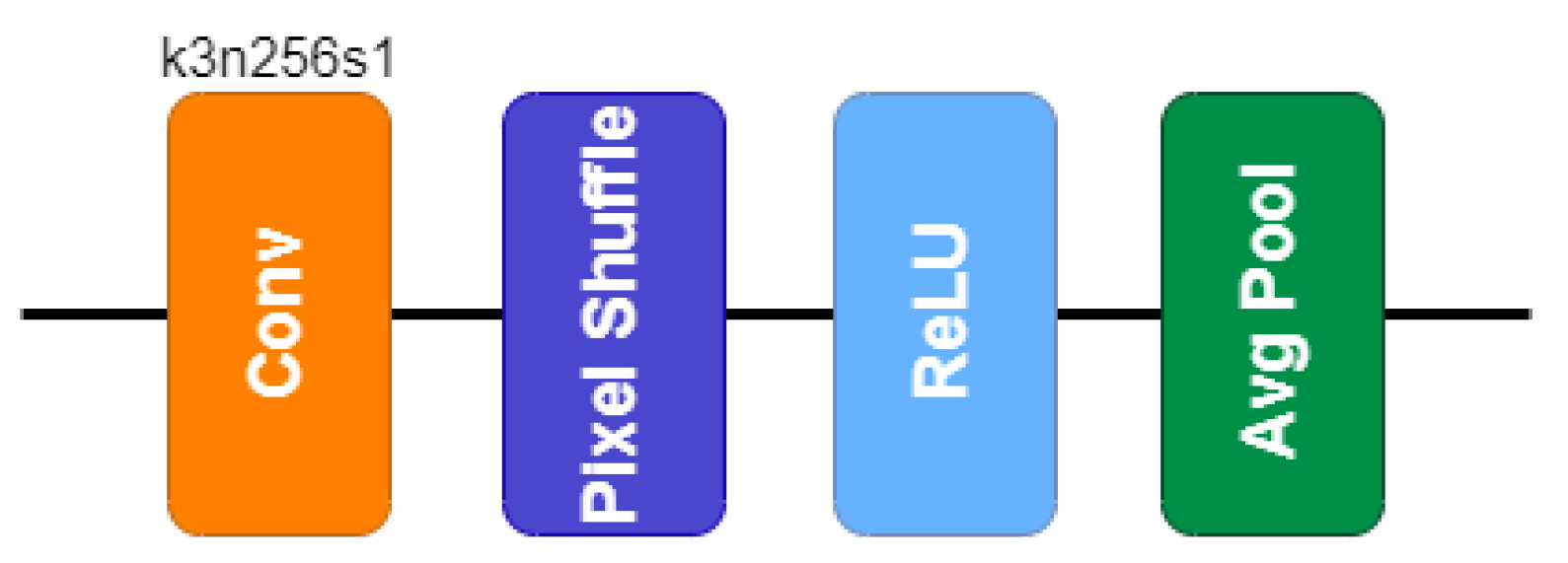
Finally, regarding the upsampling layer, Ledig et al. [14] proposed using a layer formed by a convolution, a Pixel Shuffle operator and a ReLU activation. The Pixel Shuffle operator upscales the pixel of an image by a factor of two. So, in order to achieve the $4\times$ super-resolution, the upsampling layer is applied twice.

3. Materials and Methods

3.1. Proposal

The agri-food sector is one of the engines of the Navarre’s economy. The European Commission published the Green Deal in 2019, which was followed by two strategies that will have a great impact in the coming years: the Biodiversity Strategy and the “From Farm to Fork” Strategy. The latter deals with the transition of the European food system towards an economically, socially and environmentally sustainable system, and is the one that will mark the path of many of the policies that affect the agri-food sector, including the new Common Agricultural Policy (CAP). This strategy will lead the sector to adopt measures for a more sustainable production from an environmental point of view, achieving reductions in the use of phytosanitary products and mineral fertilizers and promoting an increase in organic production and the digitization of the food chain.

NAITEC is a Technology Centre specialized in mechatronics. Thus, it wants to provide professional farmers, advisers and organizations with a tool which allows them to understand the evolution of crops in order to make predictive and precise decisions regarding their management, saving costs and reducing their environmental footprint.

It is well known that, from Sentinel images, it is possible to calculate vegetation indices such as the Normalized Difference Water Index (NDWI), the Normalized Difference Vegetation Index (NDVI) and the Normalized Difference Snow Index (NDSI) that are already being incorporated in different agricultural management software.

With this in mind, we propose a new model for super-resolution which is specifically designed to work with multispectral images. This differentiates us from the state-of-the-art models, since these are designed to work with RGB images. Additionally, our model incorporates the idea of channel attention, which takes advantage of the spatial correlations between bands. The result of this strategy is a model that not only meets its super-resolution purpose, but also exceeds the state-of-the-art methods presented so far.

3.2. Satellite Images

The Copernicus program [27] is a joint initiative of the European Commission, the Member States, the European Space Agency (ESA), the European Organization for the Exploitation of Meteorological Satellites (EUMETSAT), the European Centre for Medium Range Weather Forecasts (ECMWF), the EU Agencies and the Mercator Ocean. Such a program provides operational information about our planet captured from space, which is useful for multiple security and environmental applications. The information services are free and openly accessible to users.

In this context, five different Earth observation missions, called Sentinels [4], have been planned to guarantee the provision of data. Sentinel-2 is a mission with a constellation of two multispectral polar-orbiting satellites monitoring the Earth. It provides images for several applications, such as the study of vegetation, soil or water.

The constellation is based on two identical satellites (Sentinel-2A and Sentinel-2B) located on the same orbit and separated by 180º for optimal coverage of the Earth. The first Sentinel-2 satellite was launched on 23 June 2015.These satellites have a Multispectral Instrument (MSI) with 13 spectral bands.

Table 1. Spectral characteristics of Sentinel-2 satellites.

Spectral Bands	Sentinel-2A		Sentinel-2B
	Wavelength (nm)	Spatial Resolution (m)	Wavelength (nm)	Spatial Resolution (m)
B1—Coastal Aerosol	442.7	60	442.3	60
B2—Blue	492.4	10	492.1	10
B3—Green	559.8	10	559.0	10
B4—Red	664.6	10	665.0	10
B5—Red-edge 1	704.1	20	703.8	20
B6—Red-edge 2	740.5	20	739.1	20
B7—Red-edge 3	782.8	20	779.7	20
B8—NIR 1	832.8	10	833.0	10
B8A—NIR 2	864.7	20	864.0	20
B9—Water Vapor	945.1	60	943.2	60
B10—SWIR/Cirrus	1373.5	60	1376.9	60
B11—SWIR 1	1613.7	20	1610.4	20
B12—SWIR 2	2202.4	20	2185.7	20

shows the spatial and spectral characteristics of Sentinel-2A and Sentinel-2B satellites.

Sentinel-2 images can be obtained through the “Copernicus Open Access Hub” platform [28]. This provides access to images from the constellations Sentinel-1, Sentinel-2, Sentinel-3 and Sentinel-5P.

The other satellite we have used for the task of super-resolution is PlanetScope, a constellation of approximately 130 satellites operated by Planet [5]. It has a coverage of 200 million ${\mathrm{km}}^2$ per day, which makes it capable of covering the entire Earth’s surface daily. Its multispectral cameras capture four bands (Blue, Green, Read and Near-Infrared) and the ortho tile product GeoTIFFs are resampled at 3.125 m. It has operated since 2017, after the successful launches of 88 Dove satellites in February and of a further 48 Dove satellites in July.

3.3. Dataset

One of the main problems when trying to super-resolve the Sentinel-2 10 m spectral bands is that there are not images of this satellite to use as ground truth. To overcome this problem, two main solutions have been proposed:

• For a $2\times$ super-resolution, a model to super-resolve Sentinel-2 20 m bands to 10 m is trained and it is used for super-resolving from 10 m to 5 m [29,30].
• A high-resolution satellite as similar as possible to Sentinel-2 is selected and it is then used as ground truth [19,20,25].

Nevertheless, learning 5 m images features from 10 m ones gives very poor results, because the high-level components of a 5 m resolution cannot be found in a 10 m image. Therefore, the models are not capable of generalizing. For this reason, we have decided to find a satellite as similar as possible to the one we want to super resolve. The PlanetScope satellite is a good candidate, because its high coverage frequency allows it to find images referring to the same place and time as those of Sentinel-2. Not to mention that high-resolution satellite images are very expensive and Planet offers different alternatives to obtain the images for free.

The PlanetScope’s images used in our experiments are the Ortho Tile Analytic Surface Reflectance products. These are orthorectified, radiometrically corrected and atmospherically corrected to Bottom of Atmosphere (BOA) reflectance images. This is the image processing level we are interested in, because it represents the real reflectance of the ground, removing the distortions created by the gases of the atmosphere. The images have been obtained using the “Education and Research Standard Plan” of Planet [31], which has a download quota of 5000 ${\mathrm{km}}^2$ per month.

On the other hand, the Sentinel-2 images are free to access and they are also provided as BOA reflectance images. The images we have used are the available Sentinel-2 Level-2A images.

The study focuses on Navarre. This region is committed to the use of new techniques that allow sustainable agriculture. Satellites’ data are essential to determine the state of agroecosystems, monitor vegetation and humidity in all productive areas. However, the images precision is not valid for woody crops (vines, fruit trees, etc.) or small farms such as those that abound in Navarre.

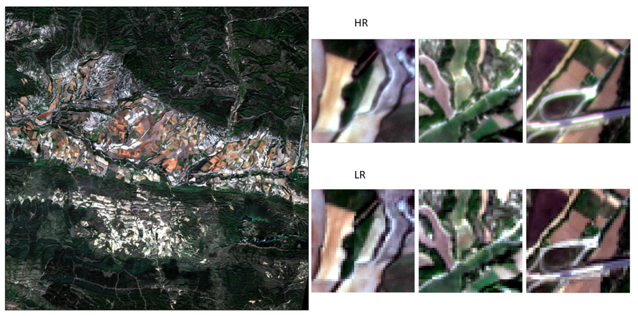
The dataset consists of 31 pairs of Sentinel-PlanetScope images that were taken in this area during the years 2020–2022. An example of the images used in the study can be seen in Figure 2. The area of study has been separated into four parts: the north-east of the region (NE), the north-west (NW), the south-west (SW) and the south-east (SE).

Table 2. Sentinel-2 and PlanetScope pairs.

Location	Date	Hour		Set	Number of Patches $2\times$	Number of Patches $4\times$
		Sentinel-2	PlanetScope
NE	06-08-2020	10:56:19	11:06:14	Train	1651	1651
	06-08-2020	10:56:19	11:06:13	Train	1180	1200
	06-08-2020	10:56:19	11:06:10	Train	1136	1131
	06-08-2020	10:56:19	11:06:10	Train	1717	1736
	06-08-2020	10:56:19	11:06:06	Test	2259	2273
	21-11-2020	10:53:49	11:00:13	Train	1407	1407
	21-11-2020	10:53:49	11:00:13	Train	2535	2538
	21-11-2020	10:53:49	11:00:08	Train	2676	2675
	07-10-2021	10:48:29	10:50:47	Train	1106	1106
	07-10-2021	10:48:29	10:50:47	Train	2698	2662
	07-10-2021	10:48:29	10:50:43	Test	2704	2650
	07-10-2021	10:48:29	10:50:40	Train	2654	2631
	07-10-2021	10:48:29	10:53:53	Validation	1763	1762
	07-10-2021	10:48:29	10:53:51	Train	2306	2280
	07-10-2021	10:48:29	10:53:49	Test	1244	1244
	07-10-2021	10:48:29	10:53:49	Train	2691	2693
	23-01-2022	11:09:16	11:31:20	Train	1259	1279
	23-01-2022	11:09:16	11:31:17	Test	842	842
NW	30-10-2020	11:02:11	11:13:25	Train	2534	2501
	30-10-2020	11:02:11	11:13:21	Validation	1994	1993
	30-10-2020	11:02:11	11:13:21	Test	722	743
	30-10-2020	11:02:11	11:13:18	Test	1286	1300
	05-09-2021	10:56:21	10:57:15	Train	2652	2704
	05-09-2021	10:56:21	10:57:15	Test	998	988
SW	22-07-2021	10:56:21	10:34:19	Validation	2469	2487
	22-07-2021	10:56:21	10:34:16	Train	2480	2459
	16-08-2021	10:56:21	10:40:59	Train	1678	1697
	18-04-2021	10:56:11	10:58:49	Test	1144	1144
SE	19-11-2021	11:09:28	10:52:06	Test	1506	1502
	19-11-2021	11:09:28	10:52:06	Train	2537	2552
	19-11-2021	11:09:28	10:52:06	Validation	993	993

shows the images used for the analysis and the set they have been assigned to.

3.4. Image Pre-Processing

The next step after downloading the images is to properly co-register them. The Sentinel-2 images cover a much larger area, so we crop them following the bounding box of the corresponding PlanetScope image. However, since the images come from two different sensors, some misregistrations still exist. In order to correct them, we use the publicly available python package AROSICS [32], a library created to perform automatic subpixel co-registration of two satellite images. Before the corrections, the PlanetScope images are resampled to 5 m resolution for the case of $2\times$ and to 2.5 m resolution for the case of $4\times$ using bicubic interpolation [6].

Next, the PlanetScope images are divided in patches of $96\times 96$ and $192\times 192$ for $2\times$ and $4\times$ super-resolution, respectively, while the images of Sentinel-2 are divided in patches of $48\times 48$. We obtain 56,821 pairs of patches for $2\times$ super-resolution and 56,823 for $4\times$ super-resolution.

Histogram Matching [33] is applied to the PlanetScope patches to match with the corresponding Sentinel-2 images, while maintaining the high-frequency components. This is a very common pre-processing step used in many computer vision tasks, and in particular it has already been used in super-resolution tasks for remote sensing [19]. Additionally, in Section 5 we show that this is a fundamental step to preserve the spectral information of the original LR image. Finally, we match the PlanetScope patches to the bicubically upsampled versions of Sentinel-2 and normalize them.

3.5. Network Architecture

We propose a network for the super-resolution of multispectral satellite images named Spectral Attention Residual Network (SARNet). The model is based on SRResNet, a network proposed in [14] which introduced the use of ResBlocks [15] for SISR for the first time.

Following the argumentation given in [16], we decide to study the effects of the Batch Normalization layer [34]. As mentioned before, the authors argue that these layers reduce the flexibility of the network and increase the GPU memory for training. On the contrary, in [18] the authors find that for real super-resolution the Batch Normalization could be beneficial due to the amount of noise in the images and the small size of the datasets. After having carried out our own experiments, we conclude that this layer helps to stabilize our training process.

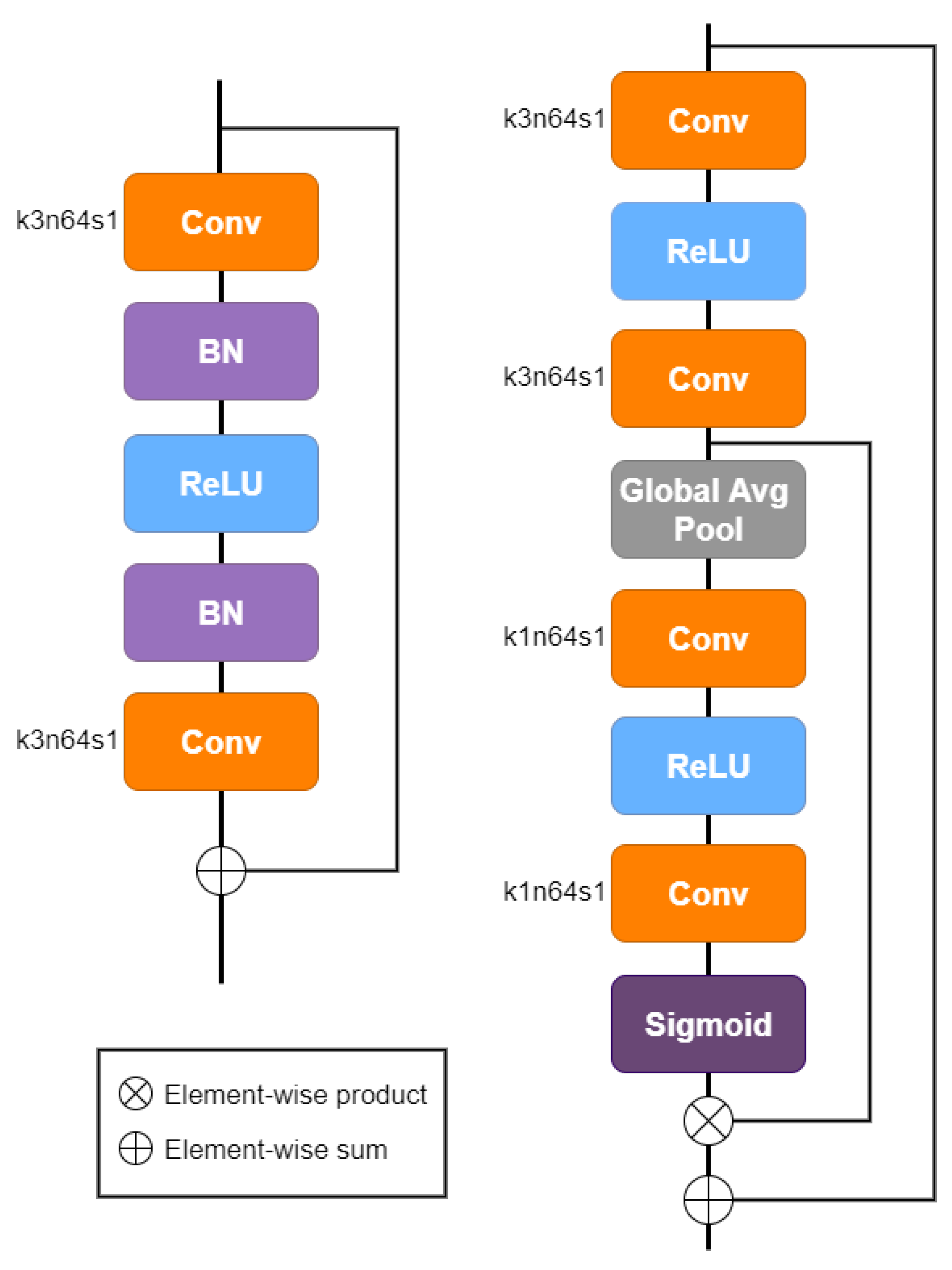
One of the main differences with respect to the SRResNet network is that, instead of the ResBlocks, we propose the use of RCAB [17], a residual block that incorporates a channel attention mechanism. The latter makes the network focus on the most informative components of the input and leads to notable performance improvements over previous state-of-the-art methods. Furthermore, the attention block is used to extract the spectral dependencies that standard residual networks are not capable of.

The architecture of a RCAB is shown in Figure 3. A Global Average Pooling is applied as an information extractor which is then passed to a channel descriptor. At the end of the block, there is a sigmoid activation followed by an element-wise multiplication to distribute the importance among channels.

With the rise of deep learning, many studies focused on the improvements achieved by increasing the depth of the models [1]. The authors of SRResNet proposed the use of 16 ResBlocks. In our experiments, a baseline model with eight RCABs is considered, but the benefit of using 16 blocks is also tested. We experimentally show in Section 4 the effects of working with a deeper network in terms of Peak Signal to Noise Ratio (PSNR) and Structural Similarity (SSIM).

After the residual blocks, we use an upsampling layer to increase the resolution of the images as in SRResNet. Each layer increases the resolution by a factor of two, so two upsampling layers are concatenated for the case of $4\times$ super-resolution. Each upsampling layer is originally formed by a convolutional layer to increase the number of filters, a Pixel Shuffle transformation to obtain a bigger image reorganizing the low-resolution image channels and a ReLU activation. Then, as proposed in [35], we introduce an Average Pooling layer for blurring the output of the Pixel Shuffle operator, in order to prevent checkerboard artifacts [36]. Our upsampling layer can be seen in Figure 4.

Finally, we introduce Short Skip Connections (SSC) inside each RCAB and a Long Skip Connection (LSC) to help stabilize the network. This way, the low-frequency information goes through the skip connections and the main network can focus on learning high-frequency information.

Our model architecture is showed in Figure 5.

3.6. Loss Function

Regarding the loss function, our starting point is the $L_1$ metric instead of the commonly used $L_2$. In [16], the authors prove that $L_1$ loss provides better convergence than $L_2$. Nevertheless, this loss function only relies on pixel-wise differences and it is not capable of capturing other important aspects based on content or style of the images. To overcome this issue, the authors of [10] propose a metric based on features extracted from the pre-trained VGG-16 network [12]. We briefly describe the VGG-16 network in order to explain our final choice.

• Pixel loss ($L_1$): The pixel loss, also known as Mean Absolute Error (MAE), is defined as the sum of the absolute differences between the pixel values of the true image Y and predicted image $\widehat{Y}$:

  $$L_1\left(Y,\widehat{Y}\right)=\frac{1}{HWC}\sum _{h=1}^H\sum _{w=1}^W\sum _{c=1}^C\left|Y_{h,w,c}-{\widehat{Y}}_{h,w,c}\right|.$$

  (1)
  Here, $H\times W$ is the size of the images and C the number of channels.
• Feature loss [10]: Instead of matching predicted image pixels with target image pixels, the feature loss (also known as content loss) encourages them to have similar feature representations. These features are usually extracted with a pre-trained VGG network. Let ${\varphi }_j\left(X\right)$ be the feature map of size $C_j\times H_j\times W_j$ of the jth convolutional layer of the VGG network when processing the image X. This loss computes the mean absolute error between the feature maps of each target image Y and predicted image $\widehat{Y}$:

  $$L_{feature}\left(Y,\widehat{Y}\right)=\frac{1}{H_j{W}_j{C}_j}{\parallel {\varphi }_j\left(Y\right)-{\varphi }_j\left(\widehat{Y}\right)\parallel }_2^2.$$

  (2)
• Style loss [10]: The style loss focuses on making the styles of the target and predicted image as similar as possible, penalizing differences in colors, textures, etc. As for feature loss, let ${\varphi }_j\left(X\right)$ be the feature map of size $C_j\times H_j\times W_j$ of the jth convolutional layer of the VGG network when processing the image X. The Gram Matrix is defined as a $C_j\times C_j$ matrix whose elements are given by:

  $$G_j^{\varphi }{\left(X\right)}_{c,c^{\prime }}=\frac{1}{H_j{W}_j{C}_j}\sum _{h=1}^{H_j}\sum _{w=1}^{W_j}{\varphi }_j{\left(X\right)}_{h,w,c}{\varphi }_j{\left(X\right)}_{h,w,c^{\prime }}.$$

  (3)
  Then, the style loss is defined as:

  $$L_{style}\left(Y,\widehat{Y}\right)={\parallel G_j^{\varphi }\left(Y\right)-G_j^{\varphi }\left(\widehat{Y}\right)\parallel }_F^2,$$

  (4)

  where ${\parallel \parallel }_F$ denotes the Frobenius norm.
• Total variation Regularization ($L_{TV}$) [10,37]: The authors of [10] justified the use of this regularizer in super-resolution tasks to favour spatial smoothness in the predicted image. However, this loss does not consider the spectral correlation between bands of multispectral and hyperspectral images. To overcome this issue, Aggarwal et al. [37] proposed a spatial–spectral total regularization. In order to reduce noise in the output images, we follow the same idea.

Finally, the loss function we propose is a combination of the previous ones. The $\alpha$, $\beta$ and $\gamma$ values in Equation (5) represents the weights.

$$L_{total}\left(Y,\widehat{Y}\right)=L_1\left(Y,\widehat{Y}\right)+\alpha L_{feature}\left(Y,\widehat{Y}\right)+\beta L_{style}\left(Y,\widehat{Y}\right)+\gamma L_{TV}\left(\widehat{Y}\right).$$

(5)

Therefore, as in the original SRResNet model, we study the benefit of using perceptual losses in the case of images coming from two different sensors. We also implement these losses with the VGG-16 network as feature extractor. The results are presented in Section 4.

3.7. Evaluation Metrics

To measure the differences between target and predicted images, two standard metrics are considered.

• Peak Signal to Noise Ratio (PSNR): PSNR is one of the most used metrics for quality evaluation of a reconstructed image. The term is used to define the relationship between the maximum possible energy of a signal and the noise that affects its faithful representation. In Equation (6), $MA{X}_Y$ corresponds to the maximum pixel value of the original image, and $MSE$ is the Mean Squared Error between the original image Y and the reconstructed image $\widehat{Y}$:

  $$PSNR\left(Y,\widehat{Y}\right)=20·lo{g}_{10}\left(\frac{MA{X}_Y}{MSE\left(Y,\widehat{Y}\right)}\right),$$

  (6)

  $$MSE\left(Y,\widehat{Y}\right)=\frac{1}{HWC}\sum _{h=1}^H\sum _{w=1}^W\sum _{c=1}^C{\left(Y_{h,w,c}-{\widehat{Y}}_{h,w,c}\right)}^2.$$

  (7)
  The error is the amount by which the values of the original image differ from the degraded image. Generally, the higher the PSNR, the better the quality of the reconstructed image.
• Structural Similarity (SSIM): SSIM is a metric that measures the similarity between two images considering the luminance, contrast and structure. It is closer to the idea that humans have of similarity. The range of the metric values is [−1,1], where 1 means that the images are identical. If Y is the original image and $\widehat{Y}$ the reconstructed image, the structural similarity between them is defined as follows:

  $$SSIM\left(Y,\widehat{Y}\right)=\frac{(2{\mu }_Y{\mu }_{\widehat{Y}}+C_1)({\sigma }_{Y,\widehat{Y}}+C_2)}{({\mu }_Y^2{\mu }_{\widehat{Y}}^2+C_1)({\sigma }_Y^2{\sigma }_{\widehat{Y}}^2+C_2)},$$

  (8)

  where ${\mu }_Y$ and ${\mu }_{\widehat{Y}}$ are the average of Y and $\widehat{Y}$, ${\sigma }_{Y,\widehat{Y}}$ is the covariance of Y and $\widehat{Y}$, ${\sigma }_Y^2$ and ${\sigma }_{\widehat{Y}}^2$ are the variances of Y and $\widehat{Y}$ and $C_1$ and $C_2$ are constants introduced to avoid instability. The latter are defined as $C_1={\left(K_{1}L\right)}^2$ and $C_2={\left(K_{2}L\right)}^2$, where L is the images maximum pixel value and $K_1$ and $K_2$ are usually set to 0.01 and 0.03, respectively.

3.8. Training Details

We train our model with Adam optimizer [38] by setting ${\beta }_1=0.9$ and ${\beta }_2=0.999$. The initial learning rate is ${10}^{-4}$ and is halved at every 25 epochs. We set the batch size as 16. The $\alpha$, $\beta$ and $\gamma$ values in Equation (5) are ${10}^{-8}$, ${10}^{-8}$ and ${10}^{-3}$, respectively. Finally, our baseline model has a total of 848 K trainable parameters for the case of $2\times$ super-resolution and 994 K for $4\times$ super-resolution.

We implement the proposed model with TensorFlow and train it using NVIDIA A100. Results are evaluated using the metrics PSNR and SSIM.

4. Results

4.1. Loss Functions

As previously mentioned, the choice of an appropriate loss function is a very important task because it can affect the results. It has been widely demonstrated that using only the $L_1$ loss function leads to blurry results [10]. Indeed, this metric depends only on low-level pixel information and is not able to retrieve high-frequency content, resulting in smooth textures [10,37]. Therefore, we investigated the most suitable metric for the task.

After some research, we chose a perceptual loss which uses the feature and style losses proposed in [10] and incorporates a total variational loss to encourage spatial and spectral smoothness in the output image.

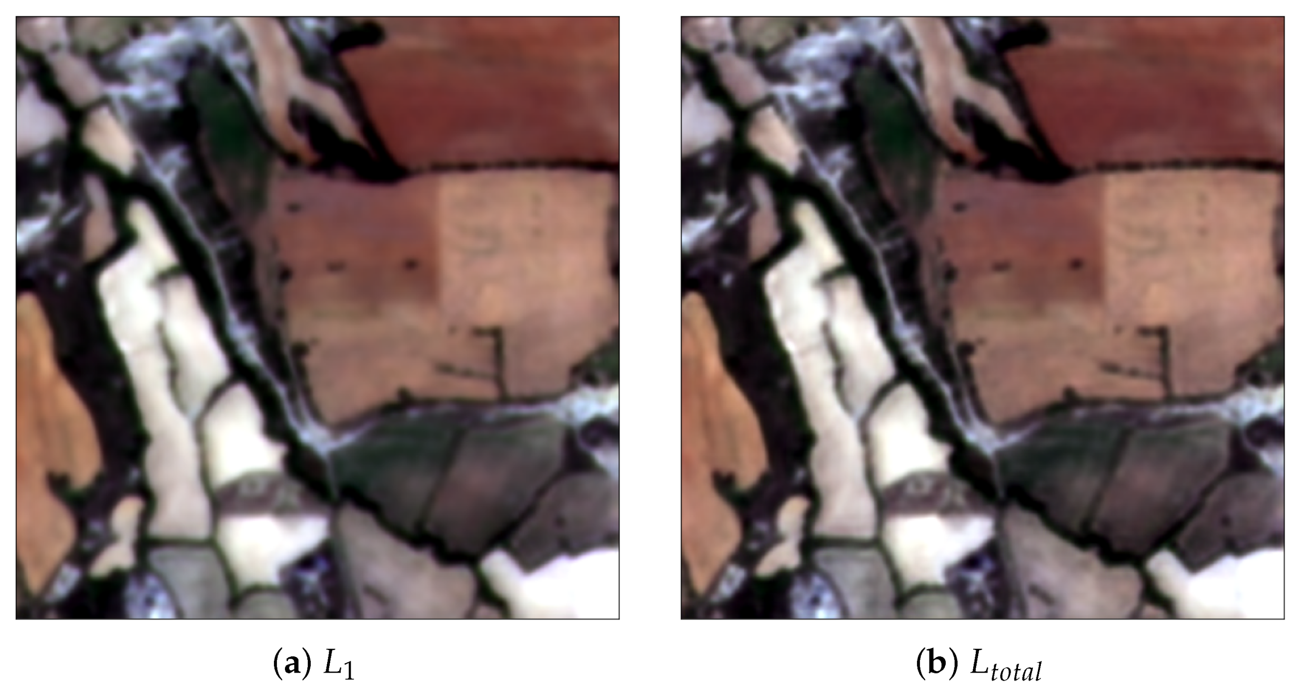
As can be seen in

Table 3. PSNR and SSIM metrics obtained for the test set with different loss functions.

Model	Loss Function	$2\times$				$4\times$
		PSNR		SSIM		PSNR		SSIM
		Mean	Std	Mean	Std	Mean	Std	Mean	Std
SARNet8	$L_1$	33.103	1.728	0.989	0.018	33.533	1.837	0.989	0.030
SARNet8	$L_{total}$	33.350	1.877	0.987	0.035	33.578	1.864	0.990	0.026

, the performances are similar. However, when visually comparing the predictions of each model, the blurring effect appears when only the $L_1$ metric is used.

Figure 6 shows the visual differences between our model trained with $L_1$ loss and trained with the proposed perceptual loss.

4.2. Depth of the Network

The objective of this section is to study the benefits of using a deeper network. We analyze two different ways of increasing the network’s depth. Firstly, we add eight more RCAB layers to the original model. Then, following the idea of residual groups used in [17], we organize the blocks into two groups of eight blocks, instead of putting them one after the other. There are two SSC in each residual group and one LSC to stabilize the training. Figure 7 shows the architecture of the second approach.

Table 4. PSNR and SSIM metrics obtained for the test set with different number of RCABs.

Model	$2\times$				$4\times$
	PSNR		SSIM		PSNR		SSIM
	Mean	Std	Mean	Std	Mean	Std	Mean	Std
SARNet8	33.350	1.877	0.987	0.035	33.578	1.864	0.990	0.026
SARNet16	33.493	1.931	0.987	0.034	33.718	1.998	0.991	0.022
SARNet16-RG	33.560	1.910	0.987	0.043	33.740	1.947	0.990	0.027

shows the results obtained with SARNet8, our baseline proposal with 8 RCABs, with SARNet16, our proposal with 16 RCABs and with SARNet16-RG, our proposal with residual groups.

We conclude that deeper models perform better, especially in terms of PSNR. Additionally, the results show that the residual group strategy helps the model learning and offers better metrics.

4.3. Comparison with Existing Models

In order to test the performance of our model, we compare it with different state-of-the-art networks, such as the well known SRCNN [8], EDSR [16] and SRResNet [14]. We also implement a simple autoencoder for image super-resolution as proposed in [24] and the commonly used bicubic interpolation.

Table 5. PSNR and SSIM metrics obtained with different models for the test set.

Model	$2\times$				$4\times$
	PSNR		SSIM		PSNR		SSIM
	Mean	Std	Mean	Std	Mean	Std	Mean	Std
Bicubic	31.218	1.510	0.979	0.018	29.471	1.320	0.936	0.046
SRCNN	31.798	1.550	0.987	0.012	31.824	1.527	0.987	0.012
Autoencoder	32.497	1.620	0.990	0.010	32.415	1.587	0.990	0.010
EDSR	32.791	1.661	0.985	0.036	32.881	1.650	0.987	0.034
SRResNet	33.001	1.706	0.985	0.040	33.197	1.741	0.989	0.024
SARNet8	33.350	1.877	0.987	0.035	33.578	1.864	0.990	0.026
SARNet16	33.493	1.931	0.987	0.034	33.718	1.998	0.991	0.022
SARNet16-RG	33.560	1.910	0.987	0.043	33.740	1.947	0.990	0.027

shows the results of the experiments.

The differences between the models in terms of SSIM are very small. This is something we expected, since the original images are very similar. Nevertheless, there is a notorious difference in the PSNR metric.

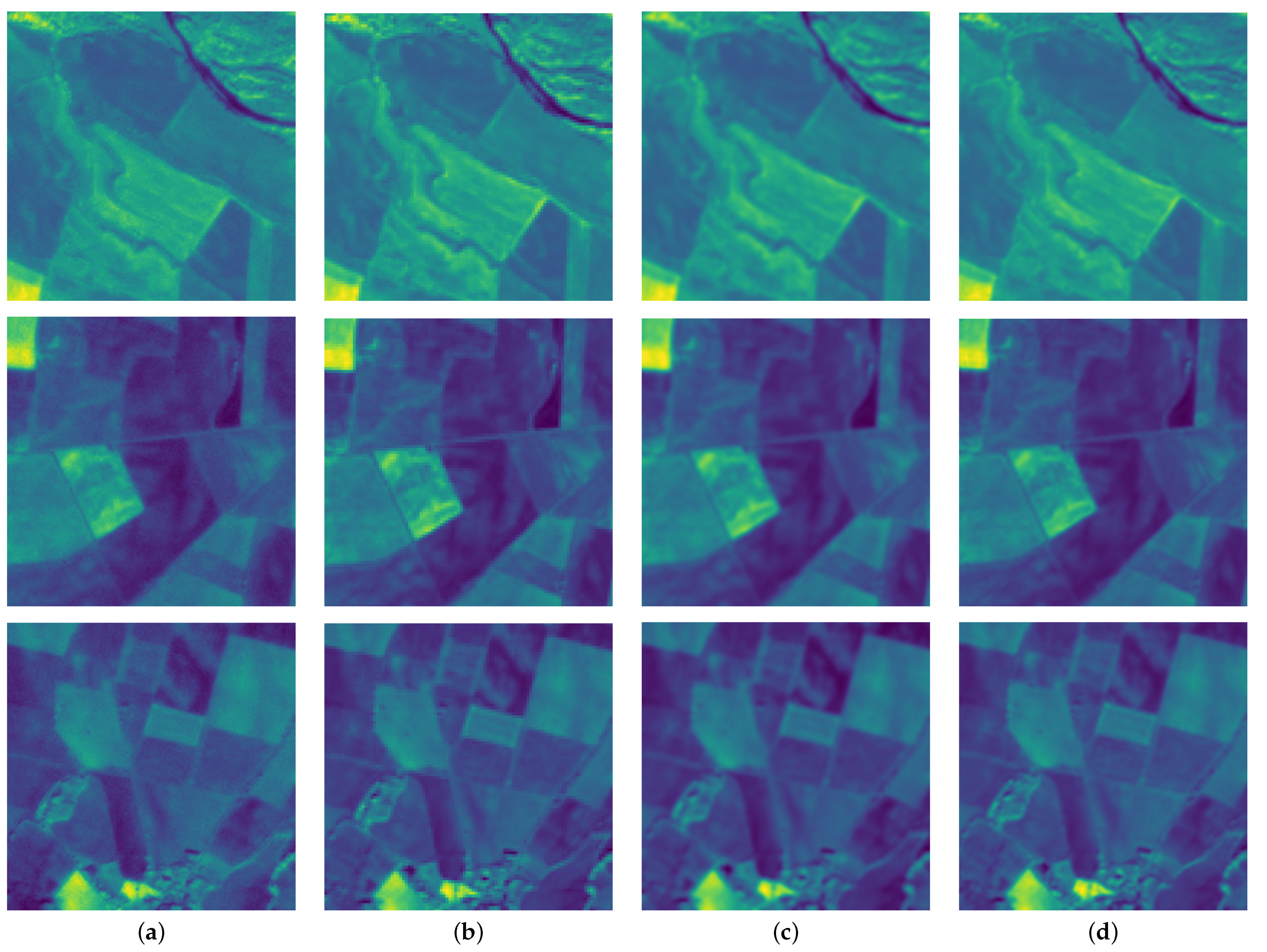
Our three proposals overpass the other state-of-the-art models. Regardless, in order to reduce computation times, we use the baseline SARNet8 model for the rest of the experiments. Figure 8 shows the visual differences between the most used interpolation methods and SARNet8. More examples are given in Appendix A.

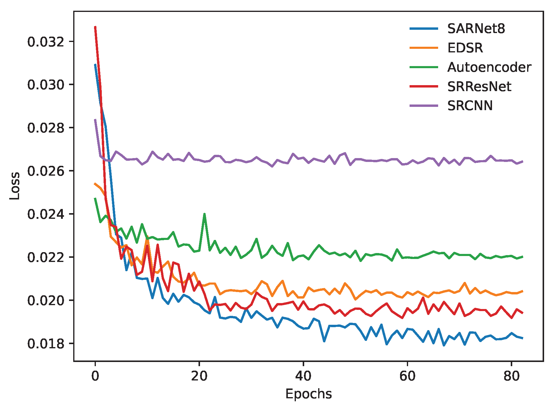
Finally, in order to gain a better sense of the models, we study their convergence. Figure 9 shows the loss curves for each model during training. Once more, SARNet8 performs better that the state-of-the-art architectures.

4.4. Spectral Validation

One of the main reasons to super-resolve Sentinel-2 images is to use them in applications where high-resolution images are needed. At the same time, the reflectance values have to be preserved while super-resolving not to alter the information provided by the image. In this section, we present the analysis to verify that the spectral content of the original image is preserved.

Figure 10 compares the LR, HR and super-resolved histograms of an image from the test set. As it can be seen, when we train our baseline model with all the pre-processing steps mentioned in Section 3 and use it to super-resolve a whole image, the histograms remain almost the same. This indicates that our model is able to maintain the reflectance values in the super-resolution process. However, when training a model without applying Histogram Matching to the PlanetScope images to match the reference Sentinel-2 images, the reflectance values of the prediction are closer to those in the PlantScope image. This shows the importance of a proper pre-processing to ensure that the original and target images are as similar as possible.

5. Conclusions and Future Work

Super-resolution of multispectral satellite images is a complex task, since usually the images come from different sensors. In this context, the pre-processing step has lot of importance. We have demonstrated that an appropriate co-registration can make a big difference in the results. For example, it avoids pixel misalignments that affect loss functions, such as $L_1$.

In this paper, we have presented a new model for the super-resolution of the RGBN bands of the Sentinel-2 Multispectral Instrument from the original 10 m to either 5 m or 2.5 m. Our model, named SARNet, has proven to be superior to the rest of state-of-the-art networks used for SISR. By incorporating a spectral channel attention mechanism, SARNet focuses on the spectral dependencies between bands, achieving improved results. We have also shown that standard loss functions such as $L_1$ fail to pay attention to the image’s perceptual characteristics, while other perceptual losses are a far better option. We have studied the benefits of using deeper models. Our results show that deeper models take advantage of skip connections in the training process. Moreover, we have ensured that the spectral information of the images is preserved after the upsampling process through Histogram Matching.

In addition, we have deal with the lack of data, one of the most common problems in deep learning. Even if there were more data, we would still take images from two different satellites. Then, the images should be as similar as possible, committing the dataset size again. Transfer learning could be a possible solution: a model is pre-trained only with images from the HR satellite, obtaining the corresponding LR images through downsampling, and then is trained with PlanetScope-Sentinel pair of images.

Another alternative is performing data augmentation, one of the most used methods when implementing a model with few data. However, the classical approach may not be the best choice for this task, mainly because the properties of the multispectral satellite images are very different from the standard RGB images used in most of the studies. The authors of [39] advise about this issue and propose different approaches for using data augmentation with satellite images.

This study focuses on Navarre, but other areas could be studied to create a more generalized model. Finally, other architectures could be analyzed. For example, GANs have proven to be a very powerful tool for the task of SISR [14,25].

References

1. Yang, W.; Zhang, X.; Tian, Y.; Wang, W.; Xue, J.; Liao, Q. Deep Learning for Single Image Super-Resolution: A Brief Review. IEEE Trans. Multimed. 2019, 21, 3106–3121. [Google Scholar] [CrossRef] [Green Version]
2. Yang, C.-Y.; Ma, C.; Yang, M.-H. Single-Image Super-Resolution: A Benchmark. In Proceedings of the European Conference on Computer Vision, Zurich, Switzerland, 6–12 September 2014; pp. 372–386. [Google Scholar]
3. Sentinel Hub. Available online: https://www.sentinel-hub.com/explore/industries-and-showcases/agriculture/ (accessed on 25 February 2022).
4. The Sentinel Missions. The European Space Agency. Available online: https://sentinel.esa.int/web/sentinel/missions (accessed on 1 October 2021).
5. Planet’s Website. Available online: https://www.planet.com/ (accessed on 9 February 2022).
6. Keys, R. Cubic Convolution Interpolation for Digital Image Processing. IEEE Trans. Acoust. Speech Signal Process. 1981, 29, 1153–1160. [Google Scholar] [CrossRef] [Green Version]
7. Chen, H.; He, X.; Wu, Y.; Ren, C.; Zhu, C. Real-World Single Image Super-Resolution: A Brief Review. Inf. Fusion. 2022, 79, 124–145. [Google Scholar] [CrossRef]
8. Dong, C.; Loy, C.C.; He, K.; Tang, X. Learning a Deep Convolutional Network for Image Super-Resolution. In Lecture Notes in Computer Science (Including Subseries Lecture Notes in Artificial Intelligence and Lecture Notes in Bioinformatics): Proceedings of the 13th European Conference, Zurich, Switzerland, 6–12 September 2014; Springer: Berlin/Heidelberg, Germany, 2014. [Google Scholar]
9. Dong, C.; Loy, C.C.; He, K.; Tang, X. Image Super-Resolution Using Deep Convolutional Networks. IEEE Trans. Pattern Anal. Mach. Intell. 2016, 38, 295–307. [Google Scholar] [CrossRef] [PubMed] [Green Version]
10. Johnson, J.; Alahi, A.; Li, F. Perceptual Losses for Real-Time Style Transfer and Super-Resolution. In Lecture Notes in Computer Science (Including Subseries Lecture Notes in Artificial Intelligence and Lecture Notes in Bioinformatics); Springer: Amsterdam, The Netherlands, 2016. [Google Scholar]
11. Kim, J.; Lee, J.K.; Lee, K.M. Accurate Image Super-Resolution Using Very Deep Convolutional Networks. In Proceedings of the IEEE Computer Society Conference on Computer Vision and Pattern Recognition, Las Vegas, NV, USA, 26 June–1 July 2016; pp. 1646–1654. [Google Scholar]
12. Simonyan, K.; Zisserman, A. Very Deep Convolutional Networks for Large-Scale Image Recognition. arXiv 2014, arXiv:1409.1556. [Google Scholar]
13. Shi, W.; Caballero, J.; Huszar, F.; Totz, J.; Aitken, A.P.; Bishop, R.; Rueckert, D.; Wang, Z. Real-Time Single Image and Video Super-Resolution Using an Efficient Sub-Pixel Convolutional Neural Network. In Proceedings of the IEEE Computer Society Conference on Computer Vision and Pattern Recognition, Las Vegas, NV, USA, 27–30 June 2016. [Google Scholar]
14. Ledig, C.; Theis, L.; Huszár, F.; Caballero, J.; Cunningham, A.; Acosta, A.; Aitken, A.; Tejani, A.; Totz, J.; Wang, Z.; et al. Photo-Realistic Single Image Super-Resolution Using a Generative Adversarial Network. In Proceedings of the 30th IEEE Conference on Computer Vision and Pattern Recognition, CVPR 2017, Honolulu, HI, USA, 21–26 July 2017; pp. 4681–4690. [Google Scholar]
15. He, K.; Zhang, X.; Ren, S.; Sun, J. Deep Residual Learning for Image Recognition. In Proceedings of the 2016 IEEE Conference on Computer Vision and Pattern Recognition (CVPR), Las Vegas, NV, USA, 26 June–1 July 2016; pp. 770–778. [Google Scholar]
16. Lim, B.; Son, S.; Kim, H.; Nah, S.; Lee, K.M. Enhanced Deep Residual Networks for Single Image Super-Resolution. In Proceedings of the IEEE Conference on Computer Vision and Pattern Recognition Workshops, Honolulu, HI, USA, 21–26 July 2017; pp. 1132–1140. [Google Scholar]
17. Zhang, Y.; Li, L.; Li, K.; Wang, L.; Zhong, B.; Fu, Y. Image Resolution Using Very Deep Residual Channel Attention Networks. arXiv 2018, arXiv:1807.02758. [Google Scholar]
18. Cheng, G.; Matsune, A.; Li, Q.; Zhu, L.; Zang, H.; Zhan, S. Encoder-Decoder Residual Network for Real Super-Resolution. In Proceedings of the IEEE/CVF Conference on Computer Vision and Pattern Recognition Workshops (CVPRW), Long Beach, CA, USA, 16–17 June 2019; pp. 2169–2178. [Google Scholar] [CrossRef]
19. Galar, M.; Sesma, R.; Ayala, C.; Albizua, L.; Aranda, C. Super-Resolution of Sentinel-2 Images Using Convolutional Neural Networks and Real Ground Truth Data. Remote Sens. 2020, 12, 2941. [Google Scholar] [CrossRef]
20. Galar, M.; Sesma, R.; Ayala, C.; Aranda, C. Super-Resolution for Sentinel-2 Images. ISPRS Int. Arch. Photogramm. Remote Sens. Spat. Inf. Sci. 2019, XLII-2/W16, 95–102. [Google Scholar] [CrossRef] [Green Version]
21. Lanaras, C.; Bioucas-Dias, J.; Galliani, S.; Baltsavias, E.; Schindler, K. Super-resolution of Sentinel-2 images: Learning a Globally Applicable Deep Neural Network. ISPRS J. Photogramm. Remote Sens. 2018, 146, 305–319. [Google Scholar] [CrossRef] [Green Version]
22. Gargiulo, M. Advances on CNN-Based Super-Resolution of Sentinel-2 Images. In Proceedings of the IGARSS 2019—2019 IEEE International Geoscience and Remote Sensing Symposium, Saint Petersburg, Russia, 1–4 July 2019. [Google Scholar]
23. Pouliot, D.; Latifovic, R.; Pasher, J.; Duffe, J. Landsat Super-Resolution Enhancement Using Convolution Neural Networks and Sentinel-2 for Training. Remote Sens. 2018, 10, 394. [Google Scholar] [CrossRef] [Green Version]
24. Müller, M.U.; Ekhtiari, N.; Almeida, R.M.; Rieke, C. Super-Resolution of Multispectral Satellite Images Using Convolutional Neural Networks. In Proceedings of the ISPRS Annals of the Photogrammetry, Remote Sensing and Spatial Information Sciences, Nice, France, 14–20 June 2020. [Google Scholar]
25. Salgueiro Romero, L.; Marcello, J.; Vilaplana, V. Super-Resolution of Sentinel-2 Imagery Using Generative Adversarial Networks. Remote Sens. 2020, 12, 2424. [Google Scholar] [CrossRef]
26. Beaulieu, M.; Foucher, S.; Haberman, D.; Stewart, C. Deep Image-To-Image Transfer Applied to Resolution enhancement of sentinel-2 images. Int. Geosci. Remote Sens. Symp. (IGARSS) 2018, 2018, 2611–2614. [Google Scholar]
27. The Copernicus Program. Available online: https://www.copernicus.eu/es (accessed on 1 October 2021).
28. Copernicus Open Acces Hub. Available online: https://scihub.copernicus.eu/dhus/#/home (accessed on 21 November 2021).
29. Wagner, L.; Liebel, L.; Körner, M. Deep Residual Learning for Single-Image Super-Resolution of Multi-Spectral Satellite Imagery. ISPRS Ann. Photogramm. Remote Sens. Spat. Inf. Sci. 2019, IV-2/W7, 189–196. [Google Scholar] [CrossRef] [Green Version]
30. Liebel, L.; Körner, M. Single-Image Super Resolution for Multispectral Remote Sensing Data Using Convolutional Neural Networks. Int. Arch. Photogramm. Remote Sens. Spat. Inf. Sci. ISPRS Arch. 2016, 41, 883–890. [Google Scholar] [CrossRef] [Green Version]
31. Eduaction and Research Program. Planet. Available online: https://www.planet.com/markets/education-and-research/ (accessed on 21 November 2021).
32. Scheffler, D.; Hollstein, A.; Diedrich, H.; Segl, K.; Hostert, P. AROSICS: An Automated and Robust Open-Source Image Co-Registration Software for Multi-Sensor Satellite Data. Remote Sens. 2017, 9, 676. [Google Scholar] [CrossRef] [Green Version]
33. Gonzalez, R.C.; Woods, R.E. Digital Image Processing, 3rd ed.; Prentice Hall: Upper Saddle River, NJ, USA, 2008. [Google Scholar]
34. Ioffe, S.; Szegedy, C. Batch Normalization: Accelerating Deep Network Training by Reducing Internal Covariate Shift. In Proceedings of the 32nd International Conference on International Conference on Machine Learning, ICML’15, Lille, France, 6–11 July 2015; Volume 37, pp. 448–456. [Google Scholar]
35. Sugawara, Y.; Shiota, S.; Kiya, H. Super-Resolution Using Convolutional Neural Networks Without Any Checkerboard Artifacts. In Proceedings of the 2018 25th IEEE International Conference on Image Processing (ICIP), Athens, Greece, 7–10 October 2018; pp. 66–70. [Google Scholar]
36. Aitken, A.; Ledig, C.; Theis, L.; Caballero, J.; Wang, Z.; Shi, W. Checkerboard Artifact Free Sub-Pixel Convolution: A Note on Sub-Pixel Convolution, Resize Convolution and Convolution Resize. arXiv 2017, arXiv:1707.02937. [Google Scholar]
37. Aggarwal, H.K.; Majumdar, A. Hyperspectral Image Denoising Using Spatio-Spectral Total Variation. IEEE Geosci. Remote Sens. Lett. 2016, 13, 442–446. [Google Scholar] [CrossRef]
38. Kingma, D.; Ba, J. Adam: A Method for Stochastic Optimization. arXiv 2014, arXiv:1412.6980. [Google Scholar]
39. Ghaffar, M.; Mckinstry, A.; Maul, T.; Vu, T.-T. Data Augmentation Approaches for Satellite Image Super-Resolution. ISPRS Ann. Photogramm. Remote Sens. Spat. Inf. Sci. 2019, IV-2/W7, 47–54. [Google Scholar] [CrossRef] [Green Version]
Figure 1. Comparison between the residual blocks in SRResNet (left) and in EDSR (right). The Batch Normalization layers from the left have been removed to create the residual blocks of EDSR (right).
Remotesensing 14 02890 g001
Figure 2. LR-HR pairs from the dataset. On the left an image from Navarre; on the right some tiles of the same image in high and low resolution.
Remotesensing 14 02890 g002
Figure 3. Comparison between the residual blocks in SRResNet (left) and RCAB in our model (right). As can be seen, the Batch Normalization layers have been removed. A channel attention block formed by a Global Average Pooling, convolution layers, a ReLU layer and a sigmoid activation function are also added.
Remotesensing 14 02890 g003
Figure 4. Upsampling layer architecture.
Remotesensing 14 02890 g004
Figure 5. Architecture of SARNet. The baseline model uses 8 RCABs followed by a convolutional layer and a batch normalization layer to stabilize the training. The upsampling block is formed by one upsampling layer in the case of 2 × super-resolution and by two upsampling layer in the case of 4 × super-resolution.
Remotesensing 14 02890 g005
Figure 6. Comparison between our baseline proposal SARNet8 trained with (a) L 1 metric and (b) L t o t a l metric. The results obtained with the second approach are sharper.
Remotesensing 14 02890 g006
Figure 7. Residual structure of the model using two residual groups, each of them formed by 8 residual channel attention blocks. These residual groups are followed by a convolutional layer.
Remotesensing 14 02890 g007
Figure 8. Visual comparison between images from the test set. (a) HR; (b) LR with nearest neighbour interpolation; (c) LR with bicubic interpolation; and (d) SARNet8. The results obtained with SARNet8 are clearly sharper.
Remotesensing 14 02890 g008
Figure 9. Network convergence comparison. SARNet8 provides the best results.
Remotesensing 14 02890 g009
Figure 10. Normalized histograms of the LR, HR, super-resolution applying histogram matching in the pre-processing (SR_HM) and without applying Histogram Matching (SR_Non-HM) for the four bands of an image from the north west of Navarre.
Remotesensing 14 02890 g010