Abstract
Large uncertainties exist in the available hydrology loading prediction models, and currently no consensus is reached on which loading model is superior or appears to represent nature in a more satisfactory way. This study discusses the noise characterization and combination of the vertical loadings predicted by different hydrology reanalysis (e.g., MERRA, GLDAS/Noah, GEOS-FPIT, and ERA interim). We focused on the hydrology loading predictions in the time span from 2011 to 2014 for the 70 Global Positioning System (GPS) sites, which are located close to the great rivers, lakes, and reservoirs. The maximum likelihood estimate with Akaike information criteria (AIC) showed that the auto-regressive (AR) model with an order from 2 to 5 is a good description of the temporal correlation that exists in the hydrology loading predictions. Moreover, significant discrepancy exists in the root mean square (RMS) of different hydrology loading predictions, and none of them have the lowest noise level for the all-time domain. Principal component analysis (PCA) was therefore used to create a combined loading-induced time series. Statistical indices (e.g., mean overlapping Hadamard variance, Nash-Sutcliffe efficiency, and variance reduction) showed that our proposed algorithm had an overall good performance and seemed to be potentially feasible for performing corrections on geodetic GPS heights.
1. Introduction
Surface mass loading modeling and its potential correction on the geodetic Global Positioning System (GPS)’s heights has captured the interest of the geodetic community for many years [,,,,]. The surface mass loading predictions are often computed by using numerical procedures (e.g., spherical harmonic function and Green’s function) with the status of Earth models and the existing surface load data (e.g., atmosphere, ocean, land hydrosphere, and cryosphere) (for details, see []). However, varying model parameters (e.g., land/sea mask, ocean response, love numbers, and earth model) as well as input data have great impacts on mass loading prediction modeling []. For the atmospheric pressure loading, the maximum errors caused by the model parameters can reach the 15% level []. Moreover, error analysis of mass loading models has not been well solved yet when performing corrections on geodetic GPS heights. There is a debate currently going on in the geodetic community about the suitability of such model-based products to effectively remove signals of geophysical origins [,,,]. More recently, many researchers have focused on the validation of mass loading prediction models by statistical comparisons to global GPS time series solutions [,,,]. However, differences in the GPS processing strategy and the applied models hamper a meaningful comparison between the GPS observation and mass loading prediction models. The root mean square (RMS)-based assessment criteria, which has been often adopted in previous studies [,], is therefore insufficient to determine which loading model is superior or that appears to represent nature in a more satisfactory way. Indeed, the question about the reliability of the GPS position time series is not straight-forward to answer yet. No ‘ground truth’ is currently available for the comparison between GPS observations and mass loading prediction models. Particularly, the errors caused by orbit, phase center, and troposphere models and low-frequency multipath variations are highly correlated and cannot be quantified yet []. Local effects (e.g., bedrock thermal expansion [], pumping and artificial recharging groundwater []) may also corrupt the model validation. Additionally, the scale adjustment in a seven-parameter transformation could absorb some of the non-linear variations related to loading effects present in the vertical residual time series [], so not all seasonal variations in the GPS data reflect real physical motion. These issues are not fully considered in mass loading validation in many previous studies. Furthermore, a very broad validation involving other geodetic techniques (e.g., very long baseline interferometry (VLBI), satellite laser ranging (SLR), and Doppler Orbitography and Radio-positioning Integrated by Satellite (DORIS)) would be enough to draw conclusions. As such, the validation of mass loading prediction models is a challenging task, and currently no consensus has been reached on which loading model is superior. To solve this problem, the creation of a combined series may be a possible alternative solution from application perspectives. The three-cornered hat (TCH) method considered by Koot et al. [] in their study of various models for atmospheric angular momentum is a good example of how a combined series might be formed to reduce series-specific noise. In addition, in the absence of ground truth data, Ferreira et al. [] adopted the TCH method to assess the quality of the Gravity Recovery and Climate Experiment (GRACE) time-variable gravity-field solutions from different processing centers. However, only those time series with poorly correlated noise could benefit from the TCH approach (for details, see [,]). This assumption is not fulfilled in most cases. In this study, we revisited this idea but used the principal components analysis (PCA) to create a combined time series, and we applied our algorithm to publicly available mass loading products.
The rest of the article is structured as follows. Section 2 details the combination algorithm based on PCA. Section 3 describes the hydrology loading (HYLD) computation. Section 4 discusses the characterization of their internal noise and the creation of a combined HYLD series. Different mass loading predictions were also evaluated by comparison to the GPS network daily solutions. Section 5 concludes and outlines ideas for further work.
2. Materials and Methods
2.1. Data Fusion with Principal Components Analysis (PCA)
In the absence of a reference dataset, one can theoretically create a combined time series from existing ones with the minimal noise variance using:
where are normalized weights, which can be obtained by requiring that the noise variance of the combined series be minimal []:
where is the noise variance.
However, for the strongly correlated data set, both the variances and the covariances were largely underestimated, which verifies that the above formula is valid only for uncorrelated or poorly correlated time series (for details, see [,]). In the case of HYLD models considered in this study, though they were modeled from the independent meteorological center, their induced displacement time series cannot be considered as uncorrelated due to the possible common-mode error sources. Consequently, we tend to use PCA to create a combined time-series from different HYLD models.
Let be a set of n displacement time series predicted by different HYLD models. We standardized the sample data and diagonalized its covariance matrix C by using the singular value decomposition (SVD) technique:
where is the diagonal matrix of eigenvalues, the kth diagonal element being the kth largest eigenvalue and the kth column of E being the corresponding eigenvector. In practice, an appropriate k is generally determined with a scree plot or the criterion based on the proportion of the total variance explained by the principal components (PCs) retained in the model []. If k-PCs are retained, the correlation coefficient [] between () and PCs (here defined by ()) can be determined by:
where is the weight for in the jth PC, is the eigenvalue associated with that PC, and is the standard deviation of .
We use , which can be considered as a measure of the contribution of with respect to their combination series, to calculate the normalized weights in such a way that . Finally, we can create a combined time series by fusing the existing ones using Equation (1).
2.2. Overlapping Hadamard Variance
Due to the computational cheapness and its insensitivity to linear frequency drift, the overlapping Hadamard variance (OHVAR) in the time domain was adopted in this study to assess the noise characteristic of the HYLD time series. OHVAR has the ability of making the maximum use of a data set by forming all possible fully overlapping samples at each averaging time []. For frequency data, OHVAR is defined as:
where is the ith of M (a pre-defined parameter) fractional frequency values (or the second differences of the phase) at averaging time , where m is the averaging factor and T0 is the basic measurement interval. Consequently, power-law (PL) noise can be distinguished by the slop (herein tentatively defined as μ) of a log-log deviation curve of the standard deviation σ(τ) (i.e., the square-root of OHVAR) time regions, which can be defined as follows:
3. Modeling Hydrology Loading Displacements
We used four different publicly available loading models: (1) HYLD (soil-moisture and snow) estimated from the European Centre for Medium-Range Weather Forecasts (ECMWF) Reanalysis (ERA interim) model [] (6 h, 0.7° × 0.7°), (2) HYLD (soil-moisture, snow, and canopy water) estimated from the Global Land Assimilation Data System/National Centers for Environmental Prediction, Oregon State University, Air Force, and Hydrology Research Laboratory (GLDAS/Noah) model [] (3 h, 0.25° × 0.25°), (3) HYLD (soil-moisture, snow, and canopy) estimated from the Goddard Earth Observing System—Forward Processing for Instrument Teams (GEOS-FPIT) model [] (1 h, 0.5° × 0.625°), and (4) HYLD (soil-moisture, snow, and canopy water) estimated from the Modern-Era Retrospective Analysis for Research and Applications (MERRA) model [] (1 h, 1/2° × 2/3°). Table 1 gives all the HYDL models characteristics to improve the clarity and the comparison. Due to a much coarser resolution and being less effective on correcting GPS data [,], HYLD estimated from the National Centers for Environmental Prediction (NCEP) reanalysis model [] (1.875° × 1.875°, 24 h) was tentatively not considered in the current research. For ERAIn-HYDL and GLDAS-HYDL, we directly used the displacements available on École et Observatoire des Sciences de la Terre/Institut de Physique du Globe de Strasbourg (EOST/IPGS) loading service (http://loading.u-strasbg.fr/, accessed on 30 December 2020). For MERRA-HYDL and GEOS-FPIT-HYDL, we used the outputs from the mass loading computation software (MALO) available on the International Mass Loading Service (http://massloading.net/, accessed on 30 December 2020) []. We noted that these four HYLD models have different environmental input data, but their computation strategies are mostly the same. Permanent ice-covered regions (Greenland, Alaska, mountain glaciers, etc.) were masked out. The conservation of the total water mass was enforced by adding/removing a uniform oceanic layer, compensating any lack/excess of water over land. To facilitate the comparison with GPS data, Green’s functions [] were all computed in the center of Earth’s figure (CF) frame using the load Love numbers (LLNs) estimated from the preliminary reference Earth model (PREM) [].

Table 1.
HYLD models and their characteristics.
It is worth noting that the GRACE is also a popular technology to study terrestrial water storage anomalies [,]. However, the fundamental temporal and spatial resolution of the GRACE data is 10 days and 400 km []. As such, GRACE may be insufficient to study the hydrological loading effects at a specific GPS site. Additionally, the computation strategy is completely different from the above four HYLD models, so we tentatively did not use the GRACE dataset in our analysis.
4. Results
For comparison purposes, we averaged displacements generated from the loading models into daily samples. Limited by the environmental input data and some GPS data, the time span of daily HYLD was tentatively chosen from 1 January 2011 to 31 December 2014. According to the standard minimum data span (i.e., 2.5 years) recommended by Blewitt and Lavallée [], the time span we chose herein was long enough to perform the noise analysis and geophysical interpretations. As expected from the predicted time series, the vertical effects (e.g., annual variations) were mostly higher than the horizontal ones; we therefore only focused on the vertical component in the following comparison. As can be seen by comparing the RMS for the 70 GPS sites, which are located near great rivers, lakes, and reservoirs (see Figure 1), systematic differences were identified in our hydrological loading models. The largest RMS discrepancy can reach to ~1.8 mm due to the different input data chosen. Here, we tentatively did not perform the error analyses of these loading models because the accuracy of the surface load input data was impossible to determine []. Alternatively, we investigated the noise content of mass loading predictions in the following section.
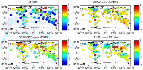
Figure 1.
RMS of displacements (in units of mm) predicted by different hydrology models in the up component for 70 GPS stations from January 2001 to December 2014. MERRA was taken as a reference to distinguish the RMS differences of the four hydrology models more clearly.
4.1. Noise Analysis
As can be seen by comparing the stacked spectra in Figure 2, possible variations near 1, 2, 3, and 4 cycles per year (cpy) can be clearly detected in HYLD. These harmonics are convincible and serve for the followed noise analysis, even though such a stacked periodogram may arbitrarily shift each individual spectra solution and its value. There are also indications that the noise in the HYLD predictions was time-correlated and the spectral index of the background noise at higher frequencies became smaller. Additionally, we used the OHVAR to obtain the noise variances as a function of time and to reflect the quality and the noise level of the series. Before performing the OHVAR, variation fits near 1, 2, 3, and 4 cpy were removed. Figure 3 gives the OHVAR results of four GPS sites (e.g., CHAN, BJFS, LHAZ, and YAR2), who had typical behavior patterns seen in all the GPS sites of the network. The results confirmed the presence of time-correlated noise in the HYLD predictions, whereas WH turned out to be unlikely or weakly to exist. We also found that the noise level was variable in time and site-by-site (the result is not provided here); thus, we could not decide which hydrology model was superior. To investigate the noise content of the HYLD models more robustly, we used the maximum likelihood estimate (MLE) method and adopted five alternative noise models in a total of seven different combinations (i.e., PL + WH, first-order autoregressive (AR(1)) + WH, second-order autoregressive (AR(2)) + WH, third-order autoregressive (AR(3)) + WH, fourth-order autoregressive (AR(4)) + WH, fifth-order autoregressive (AR(5)) + WH, and Generalized Gauss Markov (GGM) + WH, respectively) as possible descriptions of the noise. The relative goodness of fit of the noise models was tested using the Akaike information criteria (AIC) [] on a site-by-site basis (see Figure 4). We used the recently developed Hector software package [] for noise analysis and the AIC-based noise model selection. The AIC was based on the likelihood value and the number of parameter estimates. As we expected, the fraction of WH was found to be smaller than 0.05 for most sites (the result is not provided here), which agreed with the finds in the OHVAR and spectra results. Moreover, the AR noise model with an order from 2 to 5 turned out, in general, to best characterize the time-correlated noise in most HYLD predictions, whereas GGM+WH was also detected at some individual sites (see Figure 5).
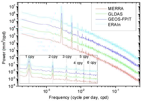
Figure 2.
Stacked periodogram of hydrology predictions for the 70 GPS sites considered. Vertical dashed lines in the zoom part indicate harmonics of about 1.0 cycle per year (cpy).
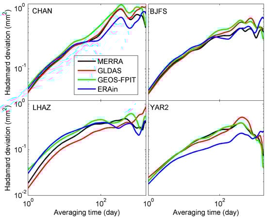
Figure 3.
Overlapping Hadamard variance of hydrology loading predictions (variation fits near 1, 2, 3, and 4 cpy were removed) at the sites of CHAN, BJFS, LHAZ, and YAR2. Error bars of Hadamard variance were omitted for clarity.
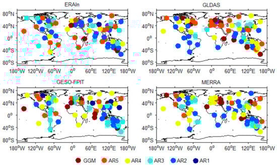
Figure 4.
Noise model scatter of the four hydrology loading predictions at 70 GPS stations for the up component with the lowest Akaike Information Criterion (AIC). AR(p) = autoregressive noise with an order of p, and GGM = Generalized Gauss Markov noise.
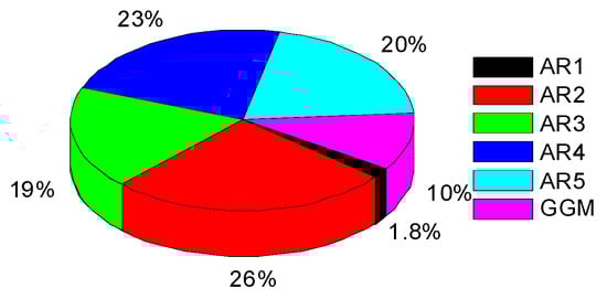
Figure 5.
The percentage of noise models in Figure 4.
4.2. Data Combining and Analysis
As mentioned above, significant discrepancy existed in the RMS of different HYLD predictions, and none of them had the lowest noise level for all time domains; we therefore constructed a combined series by making a weighted average of the existing ones in this section. In this study, those PCs with more than 90% of the cumulative variance explained by eigenvalues (see Equation (3)) were retained for normalized weight determination. Mean OHVAR during the observation time was used to evaluate the possible benefits of this combination (see Figure 6). We found that the averaged OHVARs of the combined-HYLD, MERRA-HYLD, GLDAS-HYLD, GEOS-FPIT-HYLD, and ERAIN-HYLD were 0.36, 0.41, 0.42, 0.48, and 0.33 respectively. The combined series gained an overall good OHVAR performance. The results show that the combined series had a lower noise level than MERRA-HYLD, GLDAS-HYLD, and GEOS-FPIT-HYLD, respectively, whilst the combined series had a slightly higher noise level than ERAIN-HYLD.
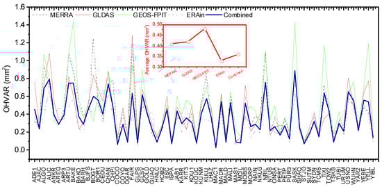
Figure 6.
Mean overlapping Hadamard variance (OHVAR) of different hydrology loading predictions and their combinations. The averaged OHVARs of 70 GPS sites were provided and inserted in the figure.
On the other hand, we made an additional comparison of the HYLD predictions with the GPS height observations. Here, we used the JPL/SOPAC combined GPS daily solutions, publicly available from the Scripps Orbit and Permanent Array Center and California Spatial Reference Center (SOPAC and CSRC) Garner GPS Archive (ftp://garner.ucsd.edu/pub/timeseries/, accessed on 30 December 2020). These daily GPS products are clean (outliers removed) and free of offset and linear trends. Solid Earth tides, polar tide, ocean tidal loading, and Earth rotation were applied in the primary GPS processing, whereas non-tidal loading (e.g., atmospheric and hydrological loading) were not yet taken into account, and they exist in the residual time series as discussed in this study. Popular indices of quantifying the accuracy of the hydrological models, such as the Nash-Sutcliffe Efficiency (NSE) [] and Weighted RMS reduction ratio in percent (WRMS%) [,], were used to indicate how well our HYLD predictions fit the GPS observations (see Figure 7). For clarity, we subtracted the non-tidal atmospheric pressure loading (ATML) and non-tidal ocean loading (NTOL) from the daily GPS time series to allow for a direct comparison with the hydrological loading. Readers should bear in mind that, currently, the uncertainties of ATML and NTOL modeling are unknown. By comparing MERRA with other updated reanalyses (e.g., ERA-Interim), advances made in this new generation of reanalyses, and archives much of the model output [,], we tentatively used the ATML from MERRA (6 h, 1/2° × 2/3°), which is calculated from the International Mass Loading Service. We also adopted the NTOL from the global Estimating the Circulation and Climate of the Oceans (ECCO) [] (12 h, about 1 degree), which were download from the EOST/IPGS loading service. The results showed that the NSE values between the GPS and HYLD were 0.09, 0.09, 0.08, 0.09, and 0.07 for the combined-HYLD, MERRA-HYLD, GLDAS-HYLD, GEOS-FPIT-HYLD, and ERAIN-HYLD, respectively. We also found that 56, 54, 53, 51, and 57 out of 70 GPS sites had their WRMS reduced for the combined-HYLD, MERRA-HYLD, GLDAS-HYLD, GEOS-FPIT-HYLD, and ERAIN-HYLD, respectively. Their averaged WRMS% reductions were 6.85%, 6.86%, 6.07%, 6.89%, and 5.23%, respectively. The results revealed that the combined-HYLD obtained more information than can be derived from a single model.
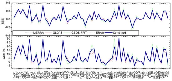
Figure 7.
Nash-Sutcliffe Efficiency (NSE) and explained variance between reduced-GPS coordinates and different hydrology loading predictions.
5. Conclusions
HYLD is a potential geophysical contributor of seasonal oscillations in GPS height observations. However, due to the earth theory problem and it being well known that the surface load data themselves can be inaccurate or incomplete, large uncertainties exist in available model-based HYLD predictions, which is significant given the current precision of geodetic observations. Temporal correlated noise was detected in HYLD predictions, which may hamper the model validation. Moreover, the noise level in HYLD predictions was variable in time and site-by-site; thus we could not decide which model was superior. To solve this problem, the creation of a combined series may be a possible alternative solution from application perspectives. This is the purpose of our paper in using a PCA-based combination method in the absence of ground truth data. We demonstrated our proposed algorithm with vertical displacements predicted by four different hydrology models (e.g., MERRA, GLDAS/Noah, GEOS-FPIT, and ERA interim) for the 70 globally distributed GPS stations. The results showed that our approach has potential applicability. We should note that our combination technique was built on purely mathematical considerations. Some critical physical issues (e.g., orography and gravity inconsistencies) were not taken into consideration. Other updated reanalyses and more quality assessments are desirable in future work to evaluate the possible benefits of the combination.
Author Contributions
C.X. and X.Y. conceived the study and carried out the noise analysis. X.H. participated in the design and coordination of the study and helped to draft the manuscript. All authors reviewed and commented on the manuscript. All authors have read and agreed to the published version of the manuscript.
Funding
This research was supported by the National Natural Science Foundation of China (41804007, 42104023) and Jiangxi University of Science and Technology High-level Talent Research Startup Project (205200100564).
Acknowledgments
We would like to acknowledge Machiel S. Bos for providing the Hector software for noise analysis. Some figures in this paper were plotted with the M_Map toolbox for Matlab [].
Conflicts of Interest
The authors declare no conflict of interest.
References
- van Dam, T.; Wahr, J.; Milly, P.C.D.; Shmakin, A.B.; Blewitt, G.; Lavallée, D.; Larson, K.M. Crustal displacements due to continental water loading. Geophys. Res. Lett. 2001, 28, 651–654. [Google Scholar] [CrossRef] [Green Version]
- van Dam, T.; Collilieux, X.; Wuite, J.; Altamimi, Z.; Ray, J. Nontidal ocean loading: Amplitudes and potential effects in GPS height time series. J. Geod. 2012, 86, 1043–1057. [Google Scholar] [CrossRef] [Green Version]
- Mémin, A.; Boy, J.-P.; Santamaría-Gómez, A. Correcting GPS measurements for non-tidal loading. GPS Solut. 2020, 24, 45. [Google Scholar] [CrossRef]
- Nicolas, J.; Verdun, J.; Boy, J.-P.; Bonhomme, L.; Asri, A.; Corbeau, A.; Berthier, A.; Durand, F.; Clarke, P. Improved Hydrological Loading Models in South America: Analysis of GPS Displacements Using M-SSA. Remote Sens. 2021, 13, 1605. [Google Scholar] [CrossRef]
- Michel, A.; Santamaría-Gómez, A.; Boy, J.-P.; Perosanz, F.; Loyer, S. Analysis of GNSS Displacements in Europe and Their Comparison with Hydrological Loading Models. Remote Sens. 2021, 13, 4523. [Google Scholar] [CrossRef]
- Van Dam, T.; Plag, H.P.; Francis, O.; Gegout, P. GGFC Special Bureau for Loading: Current status and plans. IERS Tech. Note 2003, 30, 180–198. [Google Scholar]
- Li, Y. Solid Earth Response to Environmental Variation. Ph.D. Thesis, Wuhan University, Wuhan, China, 2003. [Google Scholar]
- Petrov, L.; Boy, J.P. Study of the atmospheric pressure loading signal in VLBI observations. J. Geophys. Res. 2004, 109, B03405. [Google Scholar]
- Ray, J.; Altamimi, Z.; van Dam, T.; Herring, T. Principles for conventional contributions to modeled station displacements. In Proceedings of the IERS Conventions Workshop-Position Paper for Sessions 2 & 5, Paris, French, 22–23 September 2007; Available online: http://www.bipm.org/utils/en/events/iers/Conv_PP1.txt (accessed on 30 December 2018).
- Dach, R.; Böhm, J.; Lutz, S.; Steigenberger, P.; Beutler, G. Evaluation of the impact of atmospheric pressure loading modeling on GNSS data analysis. J. Geod. 2011, 85, 75–91. [Google Scholar] [CrossRef] [Green Version]
- Xu, C. Investigating Mass Loading Contributors of Seasonal Oscillations in GPS Observations Using Wavelet Analysis. Pure Appl. Geophys. 2016, 173, 2767–2775. [Google Scholar] [CrossRef]
- Xu, C. Evaluating mass loading products by comparison to GPS array daily solutions. Geophys. J. Int. 2017, 208, 24–35. [Google Scholar] [CrossRef]
- Li, W.; van Dam, T.; Li, Z.; Shen, Y. Annual variation detected by GPS, GRACE and loading models. Studia Geophys. Geod. 2016, 60, 608–621. [Google Scholar] [CrossRef]
- Jiang, W.; Li, Z.; van Dam, T.; Ding, W. Comparative analysis of different environmental loading methods and their impacts on the GPS height time series. J. Geod. 2013, 87, 687–703. [Google Scholar] [CrossRef]
- Dill, R.; Dobslaw, H. Numerical simulations of global-scale high-resolution hydrological crustal deformations. J. Geophys. Res. Solid Earth 2013, 118, 5008–5017. [Google Scholar] [CrossRef]
- Li, Z.; van Dam, T.; Collilieux, X.; Altamimi, Z.; Rebischung, P.; Nahmani, S. Quality Evaluation of the Weekly Vertical Loading Effects Induced from Continental Water Storage Models. In International Association of Geodesy Symposia; Springer: Berlin/Heidelberg, Germany, 2015. [Google Scholar]
- Dong, D.; Fang, P.; Bock, Y.; Cheng, M.; Miyazaki, S. Anatomy of apparent seasonal variations from GPS-derived site position time series. J. Geophys. Res. Solid Earth 2002, 107, 2075. [Google Scholar] [CrossRef] [Green Version]
- Yan, H.; Chen, W.; Zhu, Y.; Zhang, W.; Zhong, M. Contributions of thermal expansion of monuments and nearby bedrock to observed GPS height changes. Geophys. Res. Lett. 2009, 36, L13301. [Google Scholar] [CrossRef] [Green Version]
- Xiong, F.; Zhu, W. Land deformation monitoring by GPS in the Yangtze Delta and the measurements analysis. Chin. J. Geophys. 2007, 50, 1719–1730. [Google Scholar] [CrossRef]
- Collilieux, X.; Dam, T.; Ray, J.; Coulot, D.; Métivier, L.; Altamimi, Z. Strategies to mitigate aliasing of loading signals while estimating GPS frame parameters. J. Geod. 2012, 86, 1–14. [Google Scholar] [CrossRef]
- Koot, L.; Viron, O.d.; Dehant, V. Atmospheric Angular Momentum Time-Series: Characterization of their Internal Noise and Creation of a Combined Series. J. Geod. 2006, 79, 663–674. [Google Scholar] [CrossRef]
- Ferreira, V.G.; Montecino, H.; Yakubu, C.I.; Heck, B. Uncertainties of the Gravity Recovery and Climate Experiment time-variable gravity-field solutions based on three-cornered hat method. J. Appl. Remote Sens. 2016, 10, 015015. [Google Scholar] [CrossRef]
- Premoli, A.; Tavella, P. A revisited three-cornered hat method for estimating frequency standard instability. IEEE Trans. Instrum. Meas. 1993, 42, 7–13. [Google Scholar] [CrossRef]
- Jolliffe, I.T. Principal Component Analysis, 2nd ed.; Springer: New York, NY, USA, 2002; p. 488. [Google Scholar]
- Cadima, J.; Jolliffe, I.T. Loadings and correlations in the interpretation of principal components. J. Appl. Stat. 1995, 22, 203–214. [Google Scholar] [CrossRef]
- Riley, W.J. Handbook of Frequency Stability Analysis; National Institute of Standards and Technology Special Publication 1065; U.S. Department of Commerce: Washington, DC, USA, 2008; 136p.
- Dee, D.P.; Uppala, S.M.; Simmons, A.J.; Berrisford, P.; Poli, P.; Kobayashi, S.; Andrae, U.; Balmaseda, M.A.; Balsamo, G.; Bauer, P.; et al. The ERA-Interim reanalysis: Configuration and performance of the data assimilation system. Q. J. R. Meteorol. Soc. 2011, 137, 553–597. [Google Scholar] [CrossRef]
- Rodell, M.; Houser, P.R.; Jambor, U.; Gottschalck, J.; Mitchell, K.; Meng, J.; Arsenault, K.; Cosgrove, B.; Radakovich, J.; Bosilovich, M.; et al. The Global Land Data Assimilation System. Bull. Am. Meteorol. Soc. 2004, 85, 381–394. [Google Scholar] [CrossRef] [Green Version]
- Lucchesi, R. File Specification for GEOS-5 FP-IT (Forward Processing for Instrument Teams). 2013. Available online: https://ntrs.nasa.gov/citations/20150001438 (accessed on 15 April 2022).
- Reichle, R.H.; Koster, R.D.; De Lannoy, G.J.M.; Forman, B.A.; Liu, Q.; Mahanama, S.P.P.; Touré, A. Assessment and Enhancement of MERRA Land Surface Hydrology Estimates. J. Clim. 2011, 24, 6322–6338. [Google Scholar] [CrossRef] [Green Version]
- Roads, J.O.; Chen, S.C.; Kanamitsu, M.; Juang, H. Surface water characteristics in NCEP global spectral model and reanalysis. J. Geophys. Res. Atmos. 1999, 104, 19307–19328. [Google Scholar] [CrossRef]
- Petrov, L. The International Mass Loading Service. arXiv 2015, arXiv:1503.00191. [Google Scholar]
- Farrell, W. Deformation of the Earth by surface loads. Rev. Geophys. 1972, 10, 761–797. [Google Scholar] [CrossRef]
- Dziewonski, A.M.; Anderson, D.L. Preliminary reference Earth model. Phys. Earth Planet. Int. 1981, 25, 297–356. [Google Scholar] [CrossRef]
- Zhong, D.; Wang, S.; Li, J. A Self-Calibration Variance Component Model for Spatial Downscaling of GRACE Observations Using Land Surface Model Outputs. Water Resour. Res. 2020, 57, e2020WR028944. [Google Scholar] [CrossRef]
- Scanlon, B.R.; Zhang, Z.; Save, H.; Sun, A.Y.; Schmied, H.M.; Beek, L.V.; Wiese, D.N.; Wada, Y.; Long, D.; Reedy, R.C. Global models underestimate large decadal declining and rising water storage trends relative to GRACE satellite data. Proc. Natl. Acad. Sci. USA 2018, 115, E1080–E1089. [Google Scholar] [CrossRef] [Green Version]
- Rowlands, D.D.; Luthcke, S.B.; Klosko, S.M.; Lemoine, F.G.R.; Chinn, D.S.; McCarthy, J.J.; Cox, C.M.; Anderson, O.B. Resolving mass flux at high spatial and temporal resolution using GRACE intersatellite measurements. Geophys. Res. Lett. 2005, 32, L04310. [Google Scholar] [CrossRef]
- Blewitt, G.; Lavallée, D. Effect of annual signals on geodetic velocity. J. Geophys. Res. Solid Earth 2002, 107, ETG 9-1–ETG 9-11. [Google Scholar] [CrossRef] [Green Version]
- Akaike, H. Factor analysis and AIC. Psychometrika 1987, 52, 317–332. [Google Scholar] [CrossRef]
- Bos, M.; Fernandes, R.; Williams, S.; Bastos, L. Fast error analysis of continuous GNSS observations with missing data. J. Geod. 2013, 87, 351–360. [Google Scholar] [CrossRef] [Green Version]
- Nash, J.E.; Sutcliffe, J.V. River flow forecasting through conceptual models part I: A discussion of principles. J. Hydrol. 1970, 10, 282–290. [Google Scholar] [CrossRef]
- Rienecker, M.M.; Suarez, M.J.; Gelaro, R.; Todling, R.; Bacmeister, J.; Liu, E.; Bosilovich, M.G.; Schubert, S.D.; Takacs, L.; Kim, G.K.; et al. MERRA: NASA’s Modern-Era Retrospective Analysis for Research and Applications. J. Clim. 2011, 24, 3624–3648. [Google Scholar] [CrossRef]
- Decker, M.; Brunke, M.A.; Wang, Z.; Sakaguchi, K.; Zeng, X.; Bosilovich, M.G. Evaluation of the Reanalysis Products from GSFC, NCEP, and ECMWF Using Flux Tower Observations. J. Clim. 2010, 25, 1916–1944. [Google Scholar] [CrossRef]
- Wunsch, C.; Heimbach, P.; Ponte, R.M.; Fukumori, I. The Global General Circulation of the Ocean Estimated by the ECCO-Consortium. Oceanography 2009, 22, 88–103. [Google Scholar] [CrossRef]
- Pawlowicz, R. M_Map: A Mapping Package for Matlab. [Computer Software] 2020. Available online: www.eoas.ubc.ca/~rich/map.html (accessed on 30 December 2020).
Publisher’s Note: MDPI stays neutral with regard to jurisdictional claims in published maps and institutional affiliations. |
© 2022 by the authors. Licensee MDPI, Basel, Switzerland. This article is an open access article distributed under the terms and conditions of the Creative Commons Attribution (CC BY) license (https://creativecommons.org/licenses/by/4.0/).