
The Drought Events over the Amazon River Basin from 2003 to 2020 Detected by GRACE/GRACE-FO and Swarm Satellites


Abstract
:1. Introduction
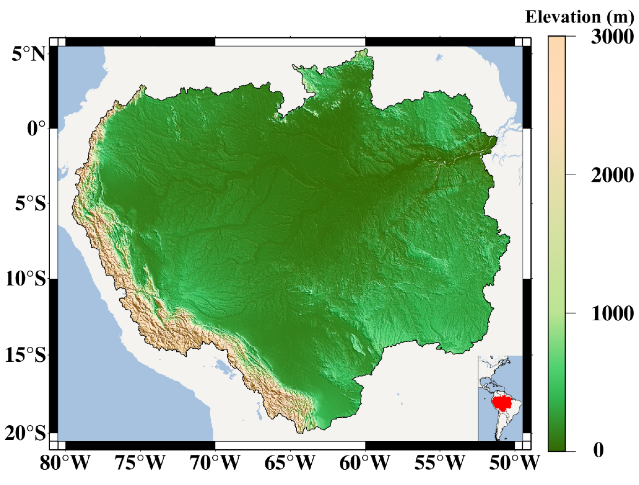
2. Study Area
3. Data
3.1. GRACE/GRACE-FO Data
3.2. Swarm Data
3.3. PPT Data
3.4. ET Data
3.5. Standardized Precipitation Evapotranspiration Index (SPEI) Data
3.6. Self-Calibrating Palmer Drought Severity Index (SCPDSI) Data
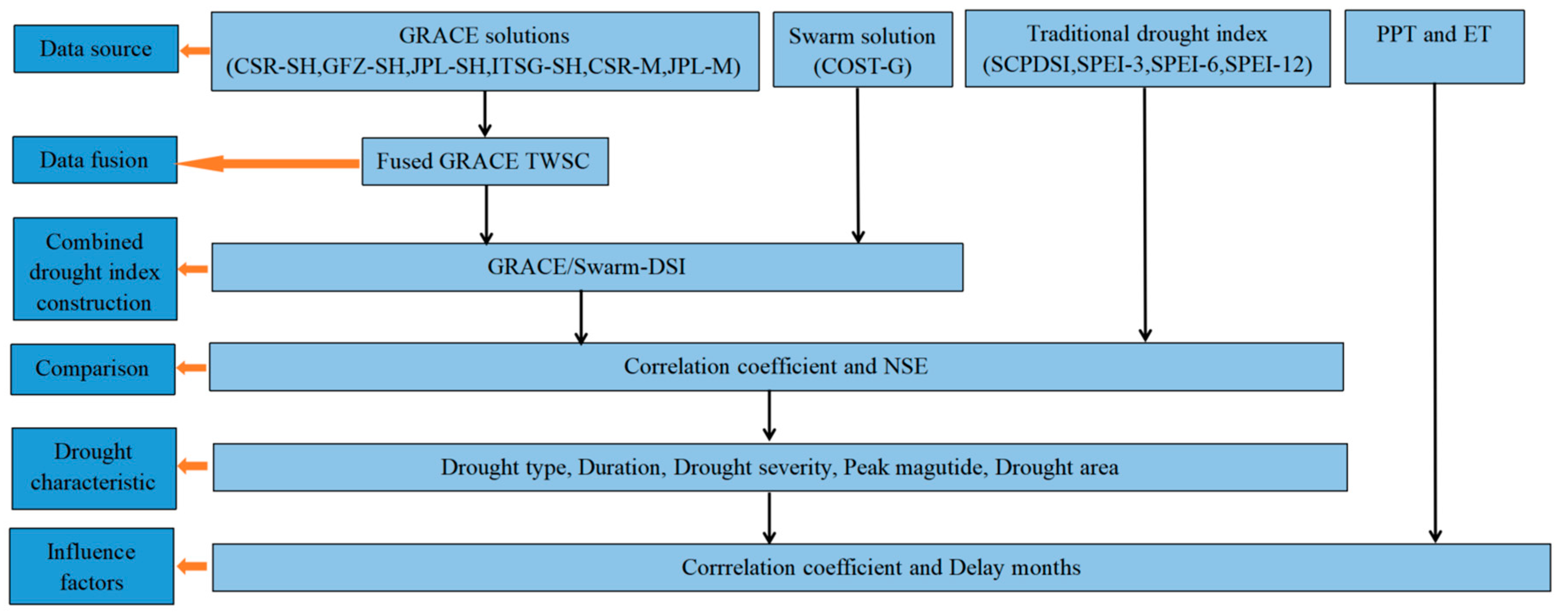
4. Method
4.1. Drought Event
4.1.1. GRACE-DSI/Swarm-DSI
4.1.2. Definition of Drought Event
4.1.3. Drought Characteristics
4.2. MSF Method
- (1)
- The gridded TWSC data were provided by the Global Land Data Assimilation system (GLDAS) the Catchment Land Surface Model (CLSM), which is the sum of soil moisture storage, snow water equivalent storage, plant canopy water and groundwater. Additionally, TWSC time series (denoted as ) in the study region was calculated by spatial averaging.
- (2)
- was split into the long-term trend items , seasonal items and residual items .
- (3)
- The original TWSC gridded data was expanded into 60-degree (GRACE) or 40-degree (Swarm) SH coefficients, and then it was converted into TWSC gridded data () using the same processing method as GRACE or Swarm data.
- (4)
- Same as the second step, was split into the long-term trend items , seasonal items and residual items .
- (5)
- According to the least square method, the scale factors of the above three signal components (, and ) were obtained, respectively.
- (6)
- The time series of TWSC from GRACE or Swarm data were also split into the long-term trend items , seasonal items and residual items .
- (7)
- The three components obtained by decomposition in step six were multiplied by the three scale factors in step five. The signal modification result is expressed by the following formula:
4.3. Different Datasets Fusion
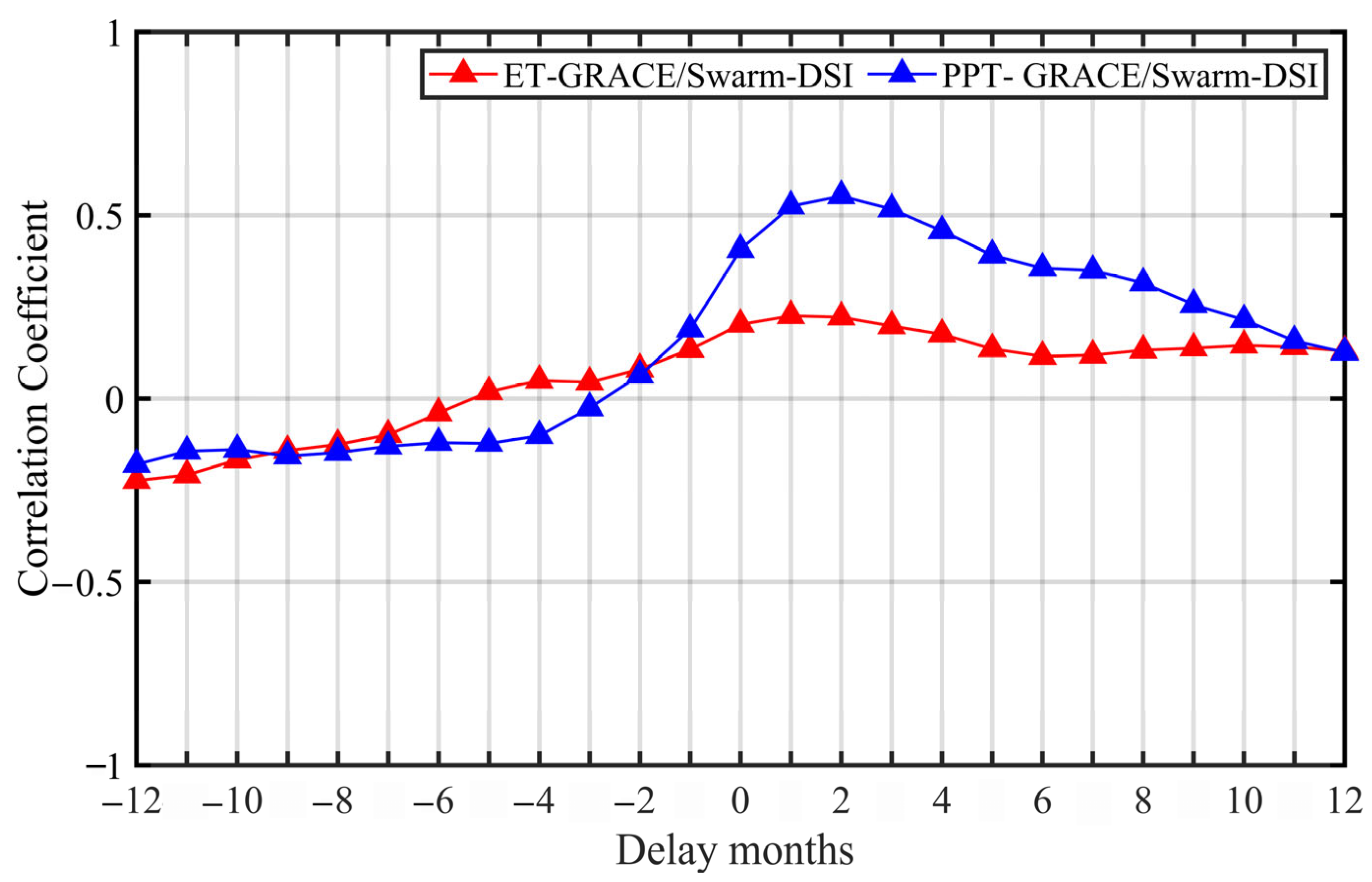
4.4. The Correlation Coefficient and Delay Months
4.5. Nash-Sutcliffe Efficiency (NSE)
4.6. Long-Term Trend Change and Acceleration
5. Results
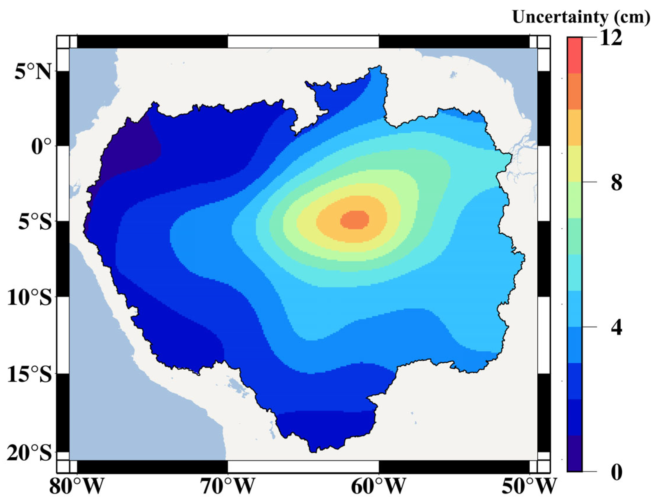
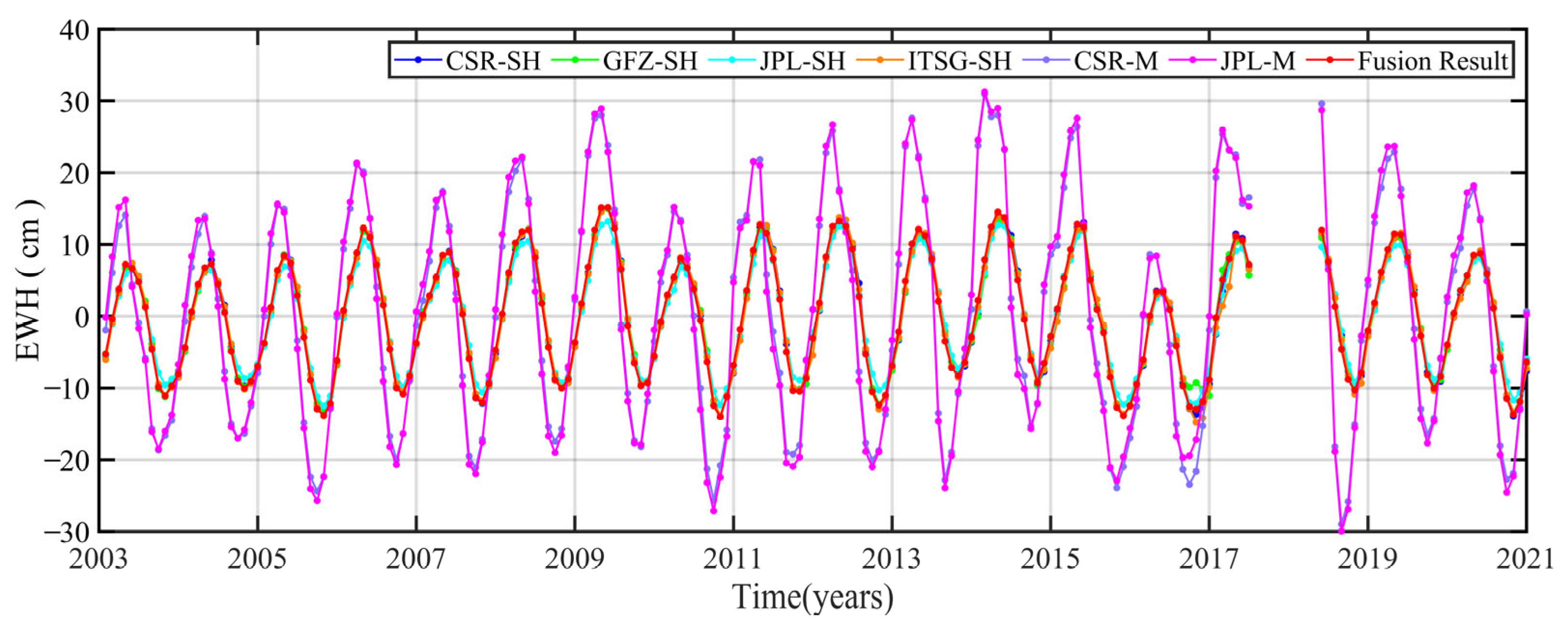
5.1. Data Fusion
5.2. Construction of the Combined Drought Index (GRACE/Swarm-DSI)
5.3. The Spatial and Temporal Change of GRACE/Swarm-DSI
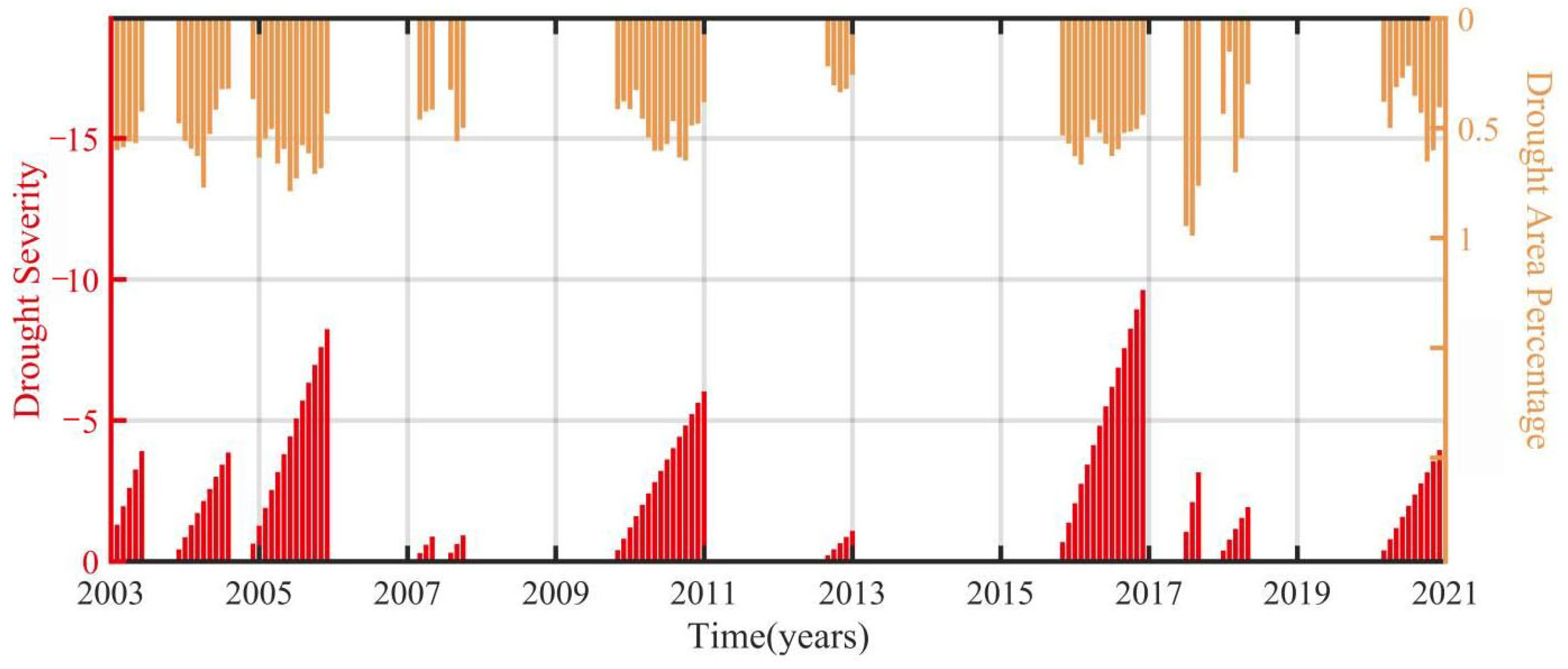
5.4. Drought Event Assessment
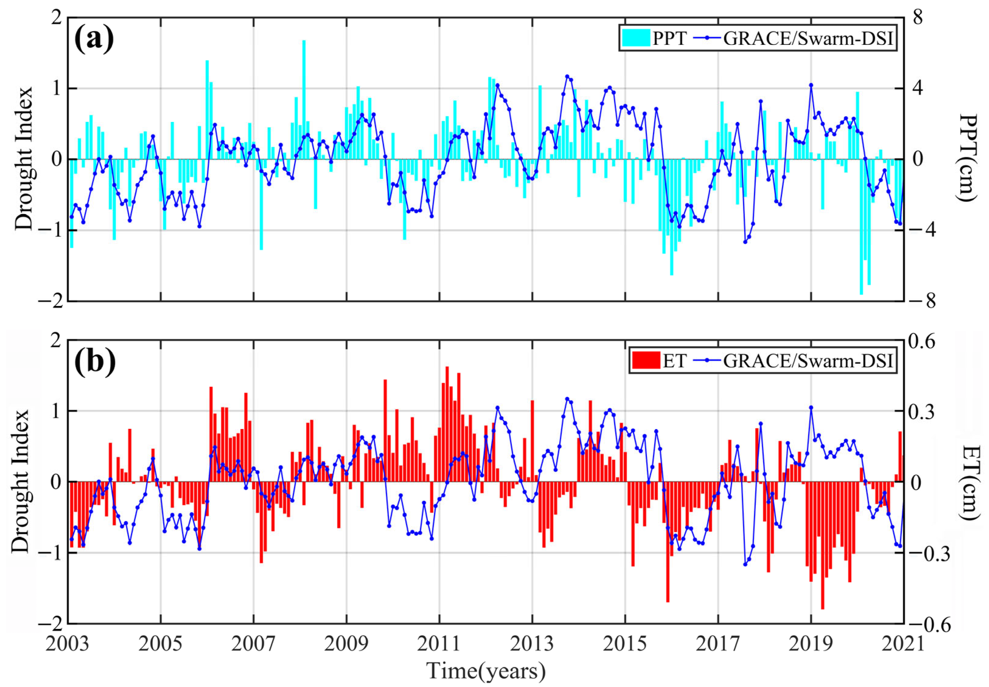
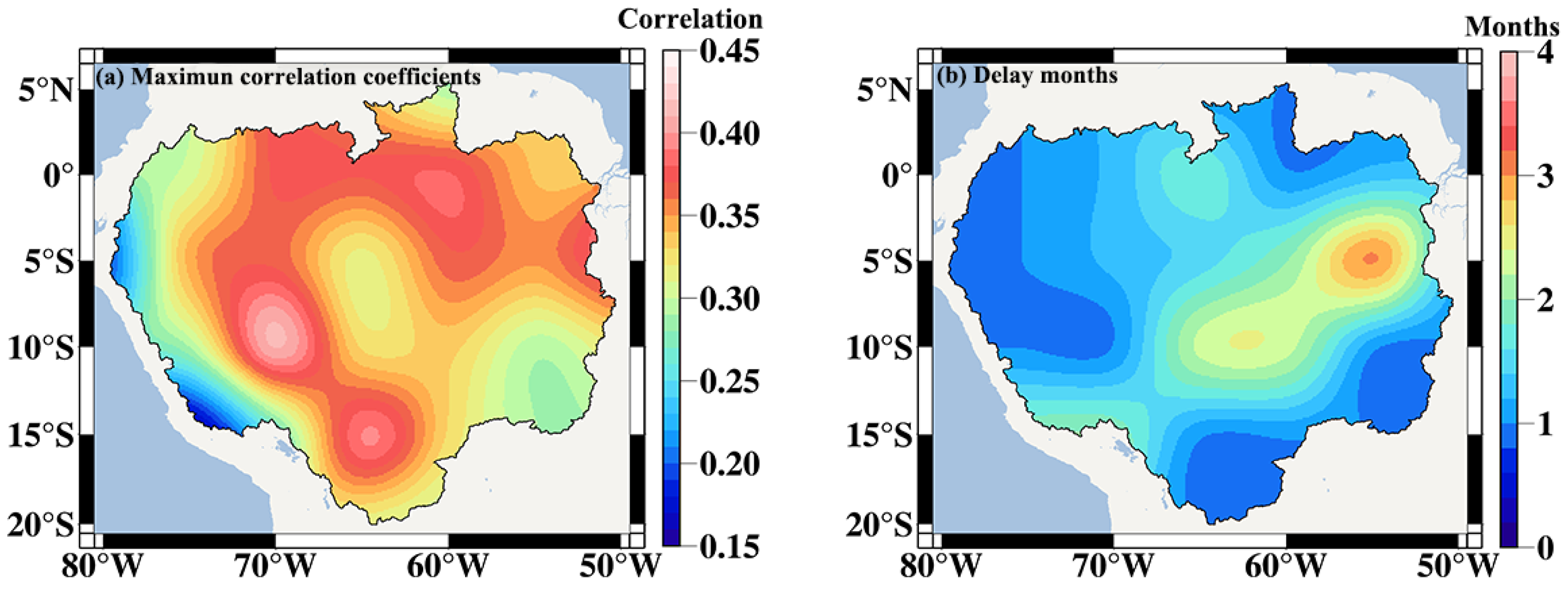
5.5. The Causes of Drought Events
6. Discussion
7. Conclusions
Author Contributions
Funding
Data Availability Statement
Acknowledgments
Conflicts of Interest
References
- Wilhite, D. Drought as a natural hazard: Concepts and definitions. Drought A Glob. Assess. 2000, 1, 3–18. [Google Scholar]
- Akyuz, D.; Bayazit, M.; Onoz, B. Markov chain models for hydrological drought characteristics. J. Hydrometeorol. 2012, 13, 298–309. [Google Scholar] [CrossRef]
- Heim, R. Review of twentieth-century drought indices used in the United State. Bull. Am. Meteorol. Soc. 2002, 83, 1149–1165. [Google Scholar] [CrossRef] [Green Version]
- Wilhite, D.; Glantz, M. Understanding the drought phenomenon: The role of definitions. Water Int. 1985, 10, 111–120. [Google Scholar] [CrossRef] [Green Version]
- Tapley, B.; Bettadpur, S.; Watkins, M.; Reigber, C. The gravity recovery and climate experiment: Mission overview and early results. Geophys. Res. Lett. 2004, 31, 09607. [Google Scholar] [CrossRef] [Green Version]
- Wahr, J.; Molenaar, M.; Bryan, F. Time variability of the Earth’s gravity field: Hydrological and oceanic effects and their possible detection using GRACE. J. Geophys. Res. 1998, 103, 30205–30229. [Google Scholar] [CrossRef]
- Li, Q.; Luo, Z.; Zhong, B.; Wang, H. Terretrial water storage change of the 2010 southwest China drought detected by GRACE temporal gravity filed. Chin. J. Geophys. 2013, 56, 1843–1849. (In Chinese) [Google Scholar]
- Cui, L.; Zhang, C.; Luo, Z.; Wang, X.; Li, Q.; Liu, L. Using the local drought data and GRACE/GRACE-FO data to characterize the drought events in Mainland China from 2002 to 2020. Appl. Sci. 2021, 11, 9594. [Google Scholar] [CrossRef]
- Tian, K.; Wang, Z.; Li, F.; Gao, Y.; Xiao, Y.; Liu, C. Drought events over the Amanzon River basin (1993–2019) as detected by the climate-driven total water storage change. Remote Sens. 2021, 13, 1124. [Google Scholar] [CrossRef]
- Vergopolan, N.; Fisher, J.B. The impact of deforestation on the hydrological cycle in Amazonia as observed from remote sensing. Int. J. Remote Sens. 2016, 37, 5412–5430. [Google Scholar] [CrossRef]
- Malhi, Y.; Roberts, J.; Betts, R.; Killeen, T.; Li, W.; Nobre, C. Climate Change, Deforestation, and the Fate of the Amazon. Science 2008, 319, 169–172. [Google Scholar] [CrossRef] [PubMed] [Green Version]
- Nobre, C.; Sellers, P.; Shukla, J. Amazonian Deforestation and Regional Climate Change. J. Clim. 1991, 4, 957–988. [Google Scholar] [CrossRef] [Green Version]
- Chaudhari, S.; Pokhrel, Y.; Moran, E.; Miguez-Macho, G. Multi-decadal hydrologic change and variability in the Amazon River basin: Understanding terrestrial water storage variations and drought characteristics. Hydrol. Earth Syst. Sci. 2019, 23, 2841–2862. [Google Scholar] [CrossRef] [Green Version]
- Chen, J.; Wilson, C.; Tapley, B.; Yang, Z.; Niu, G. 2005 drought event in the Amazon River basin as measured by GRACE and estimated by climate models. J. Geophys. Res. 2009, 114, B05404. [Google Scholar] [CrossRef]
- Frapppart, F.; Papa, F.; da Silva, J.S.; Ramillien, G.; Prigent, C.; Seyler, C.S. Surface freshwater storage and dynamics in the Amazon basin during the 2005 exceptional drought. Environ. Res. Lett. 2012, 7, 044010. [Google Scholar] [CrossRef] [Green Version]
- Nie, N.; Zhang, W.C.; Guo, H.; Ishwaran, N. 2010–2012 drought and flood events in the Amazon basin inferred by GRACE satellite observations. J. Appl. Remote Sens. 2015, 9, 096023. [Google Scholar] [CrossRef]
- Thomas, A.; Reager, J.; Famiglietti, J.; Rodell, M. A GRACE-based water storage deficit approach for hydrological drought characterization. Geophys. Res. Lett. 2014, 41, 1537–1545. [Google Scholar] [CrossRef] [Green Version]
- Da Encarnação, T.; Arnold, D.; Bezděk, A.; Dahle, C.; Doornbos, E.; van den IJssel, J.; Jäggi, A.; Mayer-Gürr, T.; Sebera, J.; Visser, P.; et al. Gravity field models derived from Swarm GPS data. Earth Planets Space 2016, 68, 127. [Google Scholar] [CrossRef] [Green Version]
- Cui, L.; Song, Z.; Luo, Z.; Zhong, B.; Wang, X.; Zou, Z. Comparison of terrestrial water storage changes derived from GRACE/GRACE-FO and Swarm: A case study in the Amazon River Basin. Water 2020, 12, 3128. [Google Scholar] [CrossRef]
- Zangerl, F.; Griesaucr, F.; Sust, M.; Montenbruck, O.; Buckert, B.; Garcia, A. SWARM GPS Precise Orbit Determination Receiver Initial In-Orbit Performance Evaluation. In Proceedings of the 27th International Technical Meeting of the Satellite Division of the Institute of Navigation, Tampa, FL, USA, 8–12 September 2014; pp. 1459–1468. [Google Scholar]
- Van den IJssel, J.; Encarnacao, J.; Doornbos, E.; Visser, P. Precise science orbit for the Swarm satellite constellation. Adv. Space Res. 2015, 56, 1042–1055. [Google Scholar] [CrossRef]
- Bezděk, A.; Sebera, J.; Teixeira da Encarnação, J.; Klokocnik, J. Time-variable gravity fields derived from GPS tracking of Swarm. Geophys. J. Int. 2016, 205, 1665–1669. [Google Scholar] [CrossRef] [Green Version]
- Jäggi, A.; Dahle, C.; Arnold, D.; Bock, H.; Meyer, U.; Beutler, G.; van den IJssel, J. Swarm kinematic orbits and gravity fields from 18 months of GPS data. Adv. Space Res. 2016, 57, 218–233. [Google Scholar] [CrossRef]
- Lück, C.; Kusche, J.; Rietbroek, R.; Löcher, A. Time-variable gravity fields and ocean mass change from 37 months of kinematic Swarm orbits. Solid Earth 2018, 9, 323–339. [Google Scholar] [CrossRef] [Green Version]
- Da Encarnação, T.; Visser, P.; Arnold, D.; Bezděk, A.; Doornbos, E.; Ellmer, M.; Guo, J.; van den IJssel, J.; Iorfida, E.; Jäggi, A.; et al. Description of the multi-approach gravity field models from Swarm GPS data. Earth Syst. Sci. Data 2020, 12, 1385–1417. [Google Scholar] [CrossRef]
- Li, F.; Wang, Z.; Chao, N.; Feng, J.; Zhang, B.; Tian, K.; Han, Y. 2015–2016 drought event in the Amazon River Basin as measured by Swarm constellation. Geomat. Inf. Sci. Wuhan Univ. 2020, 45, 595–603. (In Chinese) [Google Scholar]
- Swenson, S.; Chambers, D.; Whar, J. Estimating geocenter variations form a combination of GRACE and ocean model output. J. Geophys. Res. Solid Earth. 2008, 113, 194–205. [Google Scholar] [CrossRef] [Green Version]
- Cheng, M.; Tapley, B. Variations in the Earth’s oblateness during the past 28 years. J. Geophys. Res. 2004, 109, B09402. [Google Scholar] [CrossRef]
- Cui, L.; Zhang, C.; Yao, C.; Luo, Z.; Wang, X.; Li, Q. Analysis of the influencing factors of drought events based on GRACE data under different climatic conditions: A case study in Mainland China. Water 2021, 13, 2575. [Google Scholar] [CrossRef]
- Wang, X.; Luo, Z.; Zhong, B.; Wu, Y.; Huang, Z.; Zhou, H.; Li, Q. Separation and recovery of geophysical signals based on the kalman filter with GRACE gravity data. Remote Sens. 2019, 11, 393. [Google Scholar] [CrossRef] [Green Version]
- Jean, Y.; Meyer, U.; Jäggi, A. Combination of GRACE monthly gravity field solutions from different processing strategies. J. Geod. 2018, 92, 1313–1328. [Google Scholar] [CrossRef] [Green Version]
- Schnelder, U.; Becker, A.; Finger, P.; Meyer-Christoffer, A.; Rudolf, B.; Ziese, M. GPCC full data reanalysis version 6.0 at 2.5°: Monthly land-surface precipitation from rain-gauges built on GTS-based and historic data. GPCC Data Rep. 2011, 10, 585. [Google Scholar]
- Miralles, D.; Holmes, T.; de Jeu, R.; Gash, H.; Meesters, A.; Dolman, A. Global land surface evaporation estimated from satellite-based observations. Hydrol. Earth Syst. Sci. 2011, 15, 453–469. [Google Scholar] [CrossRef] [Green Version]
- Martens, B.; Miralles, H.; Lievens, H.; van der Schalie, R.; de Jeu, R.; Férnandez-Prieto, D.; Beck, H.; Dorigo, W.; Verhoest, N. GLEAM v3: Satellite-based land evaporation and root-zone soil moisture. Geosci. Model Dev. 2017, 10, 1903–1925. [Google Scholar] [CrossRef] [Green Version]
- Vicente-Serrano, S.; Beguería, S.; López-Moreno, J. A multiscalar drought index sensitive to global warming: The standardized precipitation evapotranspiration index. J. Clim. 2010, 23, 1696–1718. [Google Scholar] [CrossRef] [Green Version]
- Mishra, A.; Singh, V. A review of drought concepts. J. Hydrol. 2010, 391, 202–216. [Google Scholar] [CrossRef]
- Palmer, W. Meteorological Drought; US Department of Commerce: Washington, DC, USA, 1965.
- van der Schrier, G.; Barichivich, J.; Briffa, K.; Jones, P. A scPDSI-based global data set of dry and wet spells for 1901–2009. J. Geophys. Res. Atmos. 2013, 118, 4025–4048. [Google Scholar] [CrossRef]
- China Standard Press. Grades of Meteorological Drought (GB/T 20481-2017). In National Standards of People’s Republic of China; China Standard Press: Beijing, China, 2017. [Google Scholar]
- Zhao, M.; Geruo, A.; Velicogna, I.; Kimball, J.S. A global gridded dataset of GRACE drought severity index for 2002-14: Comparison with PDSI and SPEI and a case study of the Australia. J. Hydrometeorol. 2017, 18, 2117–2129. [Google Scholar] [CrossRef] [Green Version]
- Landerer, F.; Swenson, S. Accuracy of scaled GRACE terrestrial water storage estimates. Water Resour. Res. 2012, 48, W04531. [Google Scholar] [CrossRef]
- Long, D.; Yang, Y.; Wada, Y.; Hong, Y.; Liang, W.; Chen, Y.; Yong, B.; Hou, A.; Wei, J.; Chen, L. Deriving scaling factors using a global hydrological model to restore GRACE total water changes for China’s Yangtze River basin. Remote Sens. Environ. 2015, 168, 177–193. [Google Scholar] [CrossRef]
- Cui, L.; Zhu, C.; Wu, Y.; Yao, C.; Wang, X.; An, J.; Wei, P. Natural- and human- induced influences on terrestrial water storage change in Sichuan, Southwest China from 2003 to 2020. Remote Sens. 2022, 14, 1369. [Google Scholar] [CrossRef]
- Long, D.; Pan, Y.; Zhou, J.; Chen, Y.; Hou, X.; Hong, Y.; Scanlon, B.; Longuevergne, L. Global analysis of spatiotemporal variability in merged total water storage changes using multiple GRACE products and global hydrological models. Remote Sens. Environ. 2017, 192, 198–216. [Google Scholar] [CrossRef]
- Zhao, Q.; Zhang, B.; Yao, Y.; Wu, W.; Chen, Q. Geodetic and htdrological measurements reveal the recent acceleration of groundwater depletion in North China Plain. J. Hydrol. 2019, 575, 1065–1072. [Google Scholar] [CrossRef]
- Yao, C.L.; Li, Q.; Luo, Z.C.; Wang, C.R.; Zhang, R.; Zhou, B.Y. Uncertainties in GRACE-derived terrestrial water storage changes over mainland China based on a generalized three cornered hat method. Chines J. Geophys. 2019, 62, 883–897. (In Chinese) [Google Scholar]
- Cui, L.; Luo, C.; Yao, C.; Zou, Z.; Wu, G.; Li, Q.; Wang, X. The influence of climate change on forest fires in Yunnan province, Southwest China detected by GRACE satellites. Remote Sens. 2022, 14, 712. [Google Scholar] [CrossRef]
- Yan, X.; Zhang, B.; Yao, Y.B.; Yang, Y.J.; Li, J.Y.; Ran, Q.S. GRACE and land surface models reveal severe drought in eastern China in 2019. J. Hydrol. 2021, 601, 126640. [Google Scholar] [CrossRef]
- Eltahir, E.; Bras, R. Precipitation recycling. Rev. Geophys. 1996, 34, 367–378. [Google Scholar] [CrossRef]
- Lee, L.; Lawrence, D.; Price, M. Analysis of water-level response to rainfall and implications for recharge pathways in the Chalk aquifer, SE England. J. Hydrol. 2006, 330, 604–620. [Google Scholar] [CrossRef]
- Nash, J.; Sutcliffe, J. River flow forecasting through conceptual models part 1—A dicussion of pronciples. J. Hydrol. 1970, 10, 282–290. [Google Scholar] [CrossRef]
- Moriasi, D.; Arnold, J.; van Liew, M.; Bingner, R.; Harmel, R.; Veith, T. Model evalution guidelines for systematic quantification of accurary in watershed sumulation. Trans. ASABE 2007, 50, 885–900. [Google Scholar] [CrossRef]
- Werth, S.; Güntner, A.; Schmidt, R.; Kusche, J. Evaluation of GRACE filter tools from a hydrological perspective. Geophys. J. Int. 2009, 179, 1499–1515. [Google Scholar] [CrossRef] [Green Version]
- Saadi, Z.; Shahid, S.; Ismail, T.; Chung, E.; Wang, X. Trends analysis of rainfall and rainfall extreme in Sarawak, Malaysia using modified Mann-Kendall test. Meteorol. Atmos. Phys. 2019, 131, 263–277. [Google Scholar] [CrossRef]
- Gocic, M.; Trajkovic, S. Analysis of changes in meteorological variables using Mann-Kendall and Sen’s slope estimator statistical tests in Serbia. Glob. Planet. Chang. 2013, 100, 172–182. [Google Scholar] [CrossRef]
- Panisset, J.; Libonati, R.; Gouveia, C.; Machado-Silva, F.; Fança, D.; Fança, J.; Peres, L. Contrasting patterns of the extreme drought episodes of 2005, 2010 and 2015 in the Amazon basin. Int. J. Climatol. 2017, 38, 1096–1104. [Google Scholar] [CrossRef]
- 2017 Was the Second-Worst Year on Record for Tropical Tree Cover Loss. Available online: https://www.wri.org/insights/2017-was-second-worst-year-record-tropical-tree-cover-loss (accessed on 19 January 2022).
- Amazon Deforestation and Fire Update: November 2020. Available online: https://www.woodwellclimate.org/2020-amazon-deforestation-and-fire-outlook-november (accessed on 19 January 2022).
- De Silva, P.E.; Silva, C.M.S.E.; Spyrides, M.H.C.; Andrade, L.D.B. Precipitation and air temperature extremes in the Amazon and northeast Brazil. Int. J. Climatol. 2019, 39, 579–595. [Google Scholar] [CrossRef]
- Wang, Z.T.; Tian, K.J.; Li, F.P.; Xiong, S.; Gao, Y.; Wang, L.X.; Zhang, B.B. Using Swarm to detect total water storage changes in 26 global basins (taking the Amazon basin, Volga basin and Zambezi basin as examples). Remote Sens. 2021, 13, 2659. [Google Scholar] [CrossRef]
- Ndehedehe, C.E.; Ferreira, V.G. Assessing land water storage dynamics over South America. J. Hydrol. 2020, 580, 124339. [Google Scholar] [CrossRef]
- Getirana, A. Extreme Water deficit in Brazil detected from space. J. Hydrometeorol. 2016, 17, 591–599. [Google Scholar] [CrossRef]
- Sun, T.; Ferreira, V.; He, X.; Andam-Akorful, S. Water Availability of São Francisco River Basin Based on a Space-Borne Geodetic Sensor. Water 2016, 8, 213. [Google Scholar] [CrossRef]
- Cavalcante, R.; Pontes, P.; Souza, P.; De Souza, E. Opposite effects of climate and land use changes on the annual water balance in the Amazon arc of deforestation. Water Resour. Res. 2019, 55, 3092–3106. [Google Scholar] [CrossRef]


| Type | GRACE-DSI | Type | GRACE-DSI |
|---|---|---|---|
| Exceptional Drought | Moderate Drought | −1.3~−0.8 | |
| Extreme Drought | −2.0~−1.6 | Light Drought | −0.8~−0.5 |
| Severe Drought | −1.6~−1.3 | No Drought |
| SH Solution | |||
|---|---|---|---|
| CSR-GRACE | 1.171 | 1.171 | 1.000 |
| GFZ-GRACE | 1.171 | 1.171 | 1.000 |
| JPL-GRACE | 1.171 | 1.171 | 1.000 |
| ITSG-GRACE | 1.171 | 1.171 | 1.000 |
| Swarm | 1.173 | 1.173 | 1.000 |
| GRACE Solution | CSR-SH | GFZ-SH | JPL-SH | ITSG-SH | CSR-M | JPL-M | Fused Result |
|---|---|---|---|---|---|---|---|
| Medium (mm) | 43.153 | 43.628 | 44.594 | 43.315 | 107.900 | 116.491 | 36.577 |
| Correlation Coefficient | CSR-SH | GFZ-SH | JPL-SH | ITSG-SH | CSR-M | JPL-M |
|---|---|---|---|---|---|---|
| Fused results | 0.9962 | 0.9955 | 0.9957 | 0.9950 | 0.8610 | 0.8363 |
| Variables | Correlation Coefficient | NSE |
|---|---|---|
| GRACE/Swarm-DSI vs. SCPDSI | 0.6345 | 0.3348 |
| GRACE/Swarm-DSI vs. SPEI-3 | 0.5411 | 0.2783 |
| GRACE/Swarm-DSI vs. SPEI-6 | 0.6377 | 0.4044 |
| GRACE/Swarm-DSI vs. SPEI-12 | 0.6820 | 0.4627 |
| No. of Events | Time Span | Duration (Months) | GRACE/Swarm-DSI | Drought Area Percentage | Previous Studies Validation (Y/N) | ||||
|---|---|---|---|---|---|---|---|---|---|
| Peak Magnitude | Average Magnitude | Drought Severity | Peak Magnitude | Average Magnitude | Cumulative Magnitude | ||||
| 11 | 200301–200306 | 6 | −0.81 | −0.65 | −3.92 | 66.79% | 56.77% | 340.61% | Y [19] |
| 200312–200408 | 9 | −0.8 | −0.43 | −3.86 | 76.99% | 51.22% | 460.94% | Y [19] | |
| 200412–200512 | 13 | −0.98 | −0.63 | −8.24 | 78.67% | 60.28% | 783.70% | Y [15] | |
| 200703–200705 | 3 | −0.39 | −0.29 | −0.88 | 46.02% | 43.31% | 129.93% | Y [19] | |
| 200708–200710 | 3 | −0.38 | −0.31 | −0.93 | 55.89% | 46.05% | 138.15% | Y [19] | |
| 200911–201101 | 15 | −0.86 | −0.4 | −6.03 | 64.72% | 49.35% | 740.27% | Y [16,56] | |
| 201209–201301 | 5 | −0.29 | −0.22 | −1.08 | 33.67% | 28.74% | 143.72% | Y [19] | |
| 201511–201612 | 14 | −0.95 | −0.69 | −9.63 | 66.56% | 54.93% | 769.06% | Y [27] | |
| 201707–201709 | 3 | −1.16 | −1.05 | −3.16 | 98.90% | 89.91% | 269.74% | Y [57] | |
| 201801–201805 | 5 | −0.64 | −0.39 | −1.93 | 70.08% | 42.64% | 213.18% | N | |
| 202003–202012 | 10 | −0.86 | −0.39 | −3.95 | 65.05% | 41.16% | 411.62% | Y [58] | |
Publisher’s Note: MDPI stays neutral with regard to jurisdictional claims in published maps and institutional affiliations. |
© 2022 by the authors. Licensee MDPI, Basel, Switzerland. This article is an open access article distributed under the terms and conditions of the Creative Commons Attribution (CC BY) license (https://creativecommons.org/licenses/by/4.0/).
Share and Cite
Cui, L.; Yin, M.; Huang, Z.; Yao, C.; Wang, X.; Lin, X. The Drought Events over the Amazon River Basin from 2003 to 2020 Detected by GRACE/GRACE-FO and Swarm Satellites. Remote Sens. 2022, 14, 2887. https://doi.org/10.3390/rs14122887
Cui L, Yin M, Huang Z, Yao C, Wang X, Lin X. The Drought Events over the Amazon River Basin from 2003 to 2020 Detected by GRACE/GRACE-FO and Swarm Satellites. Remote Sensing. 2022; 14(12):2887. https://doi.org/10.3390/rs14122887
Chicago/Turabian StyleCui, Lilu, Maoqiao Yin, Zhengkai Huang, Chaolong Yao, Xiaolong Wang, and Xu Lin. 2022. "The Drought Events over the Amazon River Basin from 2003 to 2020 Detected by GRACE/GRACE-FO and Swarm Satellites" Remote Sensing 14, no. 12: 2887. https://doi.org/10.3390/rs14122887
APA StyleCui, L., Yin, M., Huang, Z., Yao, C., Wang, X., & Lin, X. (2022). The Drought Events over the Amazon River Basin from 2003 to 2020 Detected by GRACE/GRACE-FO and Swarm Satellites. Remote Sensing, 14(12), 2887. https://doi.org/10.3390/rs14122887