Inshore Ship Detection in Large-Scale SAR Images Based on Saliency Enhancement and Bhattacharyya-like Distance

Abstract

While the detection of offshore ships in synthetic aperture radar (SAR) images has been widely studied, inshore ship detection remains a challenging task. Due to the influence of speckle noise and the high similarity between onshore buildings and inshore ships, the traditional methods are unable to achieve effective detection for inshore ships. To improve the detection performance of inshore ships, we propose a novel saliency enhancement algorithm based on the difference of anisotropic pyramid (DoAP). Considering the limitations of IoU in small-target detection, we design a detection framework based on the proposed Bhattacharyya-like distance (BLD). First, the anisotropic pyramid of the SAR image is constructed by a bilateral filter (BF). Then, the differences between the finest two scales and the coarsest two scales are used to generate the saliency map, which can be used to enhance ship pixels and suppress background clutter. Finally, the BLD is used to replace IoU in label assignment and non-maximum suppression to overcome the limitations of IoU for small-target detection. We embed the DoAP into the BLD-based detection framework to detect inshore ships in large-scale SAR images. The experimental results on the LS-SSDD-v1.0 dataset indicate that the proposed method outperforms the basic state-of-the-art detection methods.

1. Introduction

Synthetic aperture radar (SAR) is an all-weather and all-time remote imaging sensor that has been widely used in many fields, such as ocean monitoring [1], agricultural development [2], and disaster prevention [3]. Ship detection in SAR images is of great importance in both military and commercial applications [4,5,6,7]. Although offshore ship detection in SAR images has made great progress, there are few studies on the detection of inshore ships. There are two main reasons for the difficulty of detecting inshore ships. First, the inherent speckle noise of SAR images severely affects the extraction of ship features and the accuracy of clutter statistics. Second, onshore interference objects with strong scattering intensity affect the detection accuracy of ships, such as islands, buildings, wharves, and so on.

The constant false alarm rate (CFAR) [8] detection methods are widely used in ship detection, which depend on the accurate modeling of background clutter. Novak et al. [9] proposed a two-parameter CFAR algorithm, which uses a Gaussian model to model sea clutter. Kuttikkad et al. [10] used a K-distribution to model sea clutter, and proposed the K-CFAR to detect ships. Tao et al. [11] proposed a truncated statistic-based CFAR (TS-CFAR), which can provide an accurate sea clutter modeling and a stable false alarm regulation property. However, different from offshore ships, the background clutters of inshore ships are more complex, and are difficult for existing statistical models to describe. Hence, traditional CFAR detectors are not suitable for detecting inshore ships. To this end, Zhao et al. [12] proposed an inshore ship detection method based on adaptive background windows and the CFAR with $G_0$ distribution. Wang et al. [13] proposed a maximally stable extremal region detector to extract ship candidates, and proposed an improved CFAR detector to detect inshore ships. However, due to the high similarity in scattering intensity and texture information between harbor facilities and ships, as shown in Figure 1, the above methods based on threshold segmentation are unable to achieve effective detection results on raw SAR images. In addition, the above methods ignore the influence of inherent speckle noise in SAR images, resulting in inaccurate clutter statistics.

To solve the above problems, the most direct and simplest method is to enhance the contrast between ships and background clutters. In the human visual system, the object saliency depends on its contrast rather than its brightness [14]. Zhang et al. [15] used a 2-D local-intensity-variation histogram to determine the saliency of the local region and its salient scale. Chen et al. [16] proposed a local contrast algorithm that simultaneously achieves target signal enhancement and background clutter suppression. Xie et al. [17] proposed an improved local contrast measure to obtain a saliency map, and used the level set method to achieve inshore ship detection. However, these methods usually suffer from onshore objects with high contrast, resulting in a large number of onshore false alarms. Itti et al. [18] imitated the human visual system to proposed a model of saliency-based visual attention for rapid scene analysis. The algorithm adopts a multi-scale Gaussian pyramid to express three features (intensity, color, and orientation), and uses center-surround difference to yield the saliency map. Lai et al. [19] introduced the Itti saliency model into target detection for SAR images, and used local variance, the frequency of intensity values, and global contrast to replace intensity, color, and orientation features. Wang et al. [20] selected some task-dependent scales for a Gaussian pyramid by introducing the target’s prior size information. However, for SAR images corrupted by multiplicative noise, the difference of Gaussian (DoG) cannot effectively suppress the speckle noise. In addition, Gaussian smoothing blurs the edge position, which results in the loss of important structural information. To overcome this problem, Fan et al. [21] utilized nonlinear diffusion to generate the scale space (NDSS) in SAR images, which has an advantage of preserving edges and details over the linear Gaussian scale space (GSS). Wang et al. [22] constructed an anisotropic scale space (ASS) in SAR images instead of GSS. However, the above methods do not scale the image at multiple scales, so they cannot meet the requirement of saliency enhancement for multi-scale targets. Moreover, the above methods use the differences between adjacent scales to obtain saliency maps, which will only preserve salient object edges with texture information losses, resulting in the contrast reduction of salient objects.

In recent years, deep learning-based methods have been widely used in the field of target detection and have achieved great success. Existing methods can be divided into two categories, i.e., one-stage detectors and two-stage detectors. The classic one-stage detectors include YOLO [23], SSD [24], RetinaNet [25], and so on. The classic two-stage detectors include R-CNN [26], Fast R-CNN [27], Faster R-CNN [28], Cascade R-CNN [29], and so on. To further capture ship features and suppress false alarms, some attention mechanism-based algorithms are proposed, such as the attention pyramid network [30] and feature balancing and refinement network [31]. Cui et al. [32] combined a spatial shuffle-group enhance attention module with CenterNet for ship detection in large-scale SAR images. Du et al. [33] integrated the saliency into the SSD, which can acquire refined saliency information under supervision. Furthermore, Yu et al. [34] proposed a lightweight convolution block to reduce the parameter size of the detector and speed up the training and inference. Xu et al. [35,36] realized a lightweight on-board SAR ship detector to promote the deployment of the SAR application on the satellite. However, the above methods still have some limitations in the inshore ship detection for SAR images. First, the training samples of inshore ships are too few to learn the effective features of inshore ships. Second, these top-down mechanisms depend on task specificity and require supervised training, resulting in poor generalization performance. Third, the above methods ignore the influence of inherent speckle noise in SAR images, resulting in inaccurate detection.

In addition, for large-scale SAR images, small ships usually have few pixels, which are easily ignored. Although the above deep learning-based methods have achieved great success in ship detection, these methods are unable to assign the correct positive and negative samples for small ships. The reason for this is that a slight location deviation will severely affect the intersection over union (IoU) of small ships, resulting in inaccurate positive/negative label assignments, as shown in Figure 2. The IoU of a small ship will significantly drop (from 0.79 to 0.49) when a slight location deviation occurs. Thus, the sample C of the small ship may be incorrectly assigned as a negative sample, resulting in a lack of small-ship training samples. This phenomenon implies that the sensitivity of the IoU of a small ship may cause a slight location deviation to flip the anchor label. Wang et al. [37] used the Wasserstein distance (WD) instead of IoU to achieve the positive/negative label assignment. Although the Wasserstein distance is effective for small ships, it has great limitations in large ship detection [38].

In this paper, we propose a novel inshore ship detection method in SAR images based on the difference of anisotropic pyramid (DoAP) and the Bhattacharyya-like distance-based detector (BLD). First, we propose a novel saliency enhancement algorithm based on DoAP, which can enhance the ship pixels and suppress the background clutter simultaneously. Specifically, we scale SAR images at multiple scales to construct image pyramids, and then utilize a bilateral filter (BF) to generate an anisotropic pyramid. Compared with the linear scale space built by a Gaussian kernel, the anisotropic one can reduce speckle noise and preserve more textures and details at different scales. Different from other saliency map generation algorithms that use the differences of adjacent scales, DoAP uses the differences between the finest two scales and the coarsest two scales to generate the saliency map. In addition, note that the ship pixels are located at the center of the bounding box, and the background pixels are located at the boundary of the bounding box. Therefore, a 2D Gaussian distribution can be used to represent a bounding box. Thus, the IoU of two bounding boxes can be replaced by the similarity of two Gaussian distributions. To this end, we propose replacing IoU in anchor-based detectors with the BLD for label assignment and non-maximum suppression (NMS). The value of the BLD is able to drop smoothly as the location deviation of the bounding box increases. Then, the BLD is combined with Dynamic R-CNN [39], and finally, DoAP is embedded into the BLD-based detection framework for inshore ship detection in large-scale SAR images. Experimental results on the LS-SSDD-v1.0 dataset indicate that the proposed method outperforms the state-of-the-art detection methods.

The rest of this paper is organized as follows. In Section 2 and Section 3, the related works and the proposed method are introduced. Section 4 gives the experimental results of our proposed method as well as comparisons with other state-of-the-art methods. Section 4 gives the discussion on the effectiveness of the DoAP and BLD. Finally, conclusions are given in Section 5.

2. Related Works

2.1. Anisotropic Scale Space (ASS)

Anisotropic diffusion is an adaptive filtering method that protects the meaningful details from diffusion and localization in error. The Perona–Malik (PM) [40] equation is widely used to build the ASS, which can be written as

$$I_t=div(c(x,y,t)\nabla I)=c(x,y,t)\Delta I+\nabla c·\nabla I$$

(1)

where $I_t$ is the image at scale t. $div$ represents the divergence operator, and ∇ and $\Delta$ represent gradient and Laplacian operators, respectively. $c(x,y,t)$ is the diffusion coefficient. If $c(x,y,t)$ is a constant, the anisotropic diffusion equation reduces to the isotropic heat diffusion equation. The $c(x,y,t)$ can be calculated as

$$c(x,y,t)=e^{-{\left[\left|\right|\nabla I(x,y,t)\left|\right|/K\right]}^2}$$

(2)

where the constant K can be estimated from the image gradient histogram [41]. However, the PM equation constructs the ASS in an iterative way, which is unstable and time consuming.

Wang et al. [22] analyzed the relation between the PM equation and the BF, and used the BF to replace the PM equation so as to construct the ASS quickly. The BF is defined as

$$B{F}_p=\frac{1}{k_p}\sum _{q\in S}f\left(\right||p-q|\left|\right)g\left(\right||I_p-I_q\left|\right|)$$

(3)

where q is a pixel in the neighborhood of p. $f(·)$ and $g(·)$ are spatial and intensity Gaussian kernels, respectively. $k_p$ is the normalization factor. The effect of iteration in the PM is similar to spatial Gaussian filtering, and the nonlinear diffusion is equivalent to intensity Gaussian filtering. Therefore, the BF can build the ASS fast in a noniterative way.

2.2. Dynamic R-CNN

In this paper, we adopt Dynamic R-CNN [39] as a basic detector. Generally, the threshold of the IoU for label assignment in the head networks is a fixed constant. However, positive samples from RPN networks rarely meet the fixed IoU threshold in early iterations. The Dynamic R-CNN tunes down the initial threshold T of the IoU and progressively increases it during the iteration training process to adapt to changes in the quality of proposal bounding boxes. In addition, the regression loss of high-quality samples is small, which is not conducive to model updates. Therefore, in Dynamic R-CNN, the hyper-parameter $\beta$ of the smooth L1 loss function is reduced by the prediction error to increase the gradient of high-quality samples.

We adopt ResNet50 and FPN as the backbone and neck networks, respectively, to extract deep feature maps. The feature extraction capability of ResNet as a backbone network has been demonstrated in many detectors, and FPN is also a common strategy to scope the multi-scale problem of target detection. Then, RPN is used to obtain proposal boxes from the feature maps for the reason that RoIPooling will generate quantization loss in the unified feature scale operation, which has less effect on large targets, but more on small targets. Therefore, Dynamic R-CNN adopts RoIAlign instead of RoIPooling to deal with the difference in feature scales caused by multi-scale proposal boxes. Finally, the unified scale features are input into the head networks of Dynamic R-CNN, which updates the positive sample selection threshold with the number of iterations. The head networks of Dynamic R-CNN consist of a classification branch and a location regression branch to predict the class and location of the target, respectively. The above steps can be summarized as follows:

• Feature extraction: ResNet50 and FPN are used as the backbone and neck networks, respectively, to obtain feature maps;
• Label assignment: Positive and negative samples for training RPN/R-CNN are assigned by calculating the IoU of ground truth boxes and anchor boxes/proposal boxes;
• NMS: The IoU of proposal boxes/predicted boxes is calculated to suppress overlapping boxes;
• Region proposal: RPN is used to obtain proposal boxes, which requires label assignment in the training phase and NMS during the prediction phase;
• RoIAlign: Bilinear interpolation is used to align features;
• Dynamic detection: The IoU threshold T and hyper-parameter $\beta$ of the R-CNN are adjusted gradually with the number of iterations. The R-CNN requires label assignment in the training phase and NMS during the prediction phase.

In this paper, a novel distance measure of bounding boxes, BLD, is proposed to replace IoU. The BLD is specially applied in the label assignment and NMS operations.

3. Methodology

Figure 3 gives the overall architecture of the proposed method. The proposed method consists of two parts, the DoAP and BLD-based Dynamic R-CNN. First, the final saliency enhancement result is obtained through DoAP; then, the raw SAR image and the final saliency enhancement result are jointly used as the input of the subsequent detector. Second, Dynamic R-CNN is used as the basic detection framework, where IoU in label assignment and NMS operation is replaced by the BLD. In this section, we will introduce the details and contributions of each module.

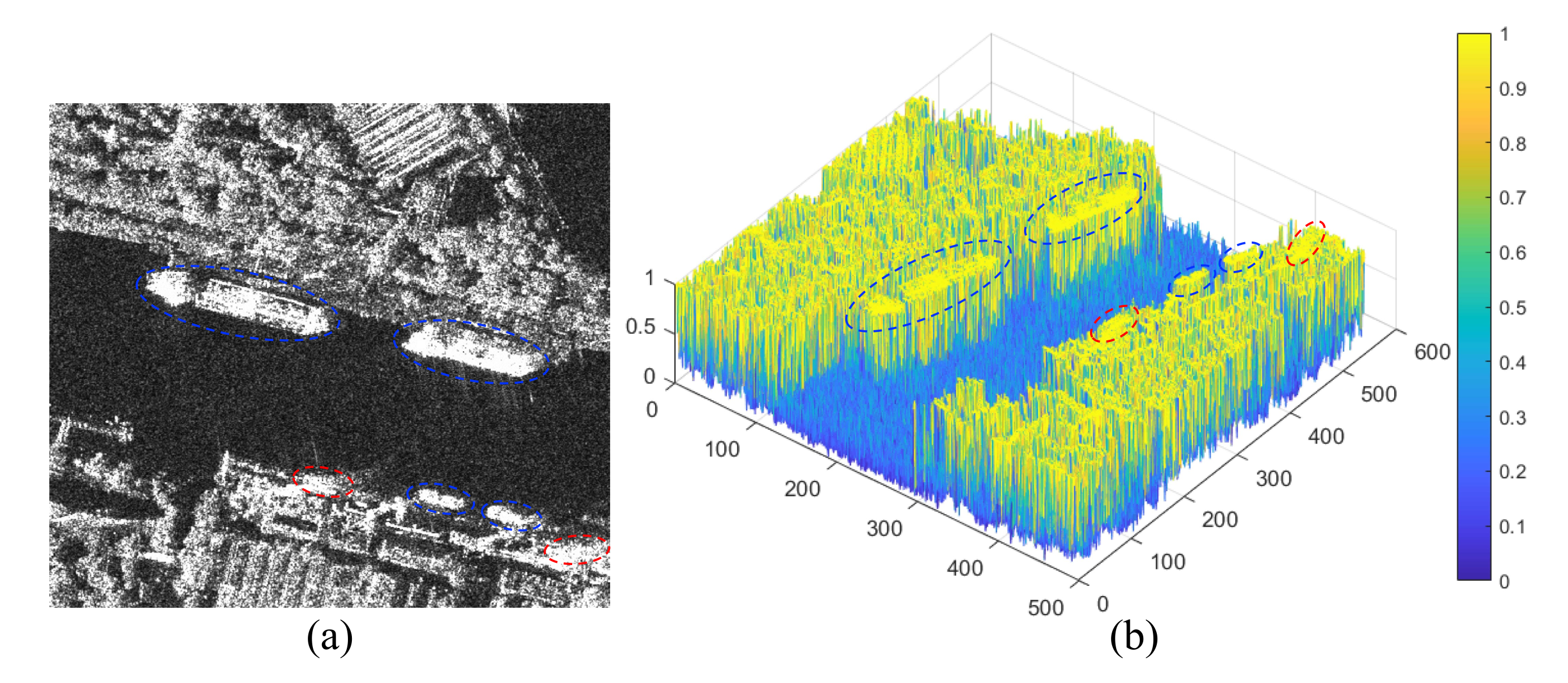
3.1. Saliency Enhancement

At present, saliency enhancement methods can be divided into two categories, i.e., top-down and bottom-up methods. The top-down methods scan the scene in a slower, volition-controlled, and task-dependent manner [42]. However, the top-down methods require task-related training samples and have poor generalization performance. The saliency-based visual attention model proposed by Itti [18] lays the foundation for bottom-up methods. Since then, many improved Itti saliency models have been proposed for the saliency enhancement of SAR images. Lai et al. [19] adopted local variance, the frequency of intensity values, and global contrast to replace the three features in an Itti saliency model. Liu et al. [43] proposed an SAR image saliency enhancement method that combines Itti’s pyramid model with singular value decomposition. However, Itti’s pyramid model is constructed by a Gaussian kernel, which blurs the edge position and loses important structural information. In this paper, we adopt the BF to construct an anisotropic pyramid instead of the Gaussian pyramid. In addition, we design a novel image difference strategy named the difference of anisotropic pyramid (DoAP). This strategy uses the differences between the finest two scales and the coarsest two scales to generate the saliency map, as shown in Figure 4. Finally, to avoid the contrast enhancement in low-scattering regions, we multiply the normalized saliency map by the SAR image as the final saliency enhancement result.

First, we adopt the bilinear interpolation algorithm to construct an image pyramid. As shown in Figure 5, the coordinates and intensities of pixels $Q_{11}$, $Q_{12}$, $Q_{21}$, and $Q_{22}$ are known; the intensity of pixel P can be computed as

$$\left\{\begin{array}{c}f\left(x,y_1\right)\approx \frac{x_2-x}{x_2-x_1}f\left(Q_{11}\right)+\frac{x-x_1}{x_2-x_1}f\left(Q_{21}\right)\hfill \\ f\left(x,y_2\right)\approx \frac{x_2-x}{x_2-x_1}f\left(Q_{12}\right)+\frac{x-x_1}{x_2-x_1}f\left(Q_{22}\right)\hfill \\ f\left(P\right)\approx \frac{y_2-y}{y_2-y_1}f\left(x,y_1\right)+\frac{y-y_1}{y_2-y_1}f\left(x,y_2\right)\hfill \end{array}\right.$$

(4)

where $f\left(X\right)$ denotes the intensity of pixel X.

Second, we adopt a BF for each image in the image pyramid to construct the anisotropic pyramid. The anisotropic pyramid can effectively reduce the negative influence of speckle noise while preserving the details and edges in each image scale. Then, we propose the DoAP to generate the saliency map of SAR images, which can enhance the ship pixels and suppress the onshore pixels. For an n-scale anisotropic pyramid ($A=\{A_1,A_2,\dots ,A_n\}$), the feature maps of the DoAP can be calculated as

$$\left\{\begin{array}{c}{F}_1=|A_1-resize\left(A_{n-1}\right)|\hfill \\ F_2=|A_2-resize\left(A_n\right)|\hfill \end{array}\right.$$

(5)

where $resize\left(A_i\right)$ denotes that $A_i$ is scaled to the same size as the minuend.

To eliminate amplitude differences, the feature maps are normalized to a fixed range [0, M]. Then, we find the location of the global maximum M for each feature map, and compute the average $\overline{m}$ of all its other local maxima. Now, the global normalization operator $\mathcal{N}(·)$ can be written as

$$\mathcal{N}\left(F\right)=F\times {(M-\overline{m})}^2$$

(6)

Next, the saliency map S is obtained through across-scale addition as

$$S=\mathcal{N}\left(F_1\right)+resize\left(\mathcal{N}\left(F_2\right)\right)$$

(7)

where $resize\left(F\right)$ means to scale F to the same size as the summand.

Note that most methods directly replace the original image with the saliency map as the input for subsequent tasks. However, for the reason that most methods utilize local contrast to enhance target saliency, non-target edges are generated in flat regions, especially in water. Therefore, the final saliency enhancement result is obtained by multiplying the raw SAR image and the normalized saliency map. Then, the raw SAR image and the final saliency enhancement result are jointly used as the input of the subsequent detector. The implementation details of the proposed DoAP are shown in Algorithm 1.

Algorithm 1 The proposed DoAp.

Input:  SAR image I, the dimension of image pyramid n. 1: Image pyramid ($IP$) $\leftarrow I{P}_0=I$. 2: for $i=2\to n$ do 3:     $I{P}_i$← Equation (4). 4: end for 5: for $i=1\to n$ do 6:     Anisotropic pyramid ($A_i$) ← BF($I{P}_i$). 7: end for 8: Feature maps $\left[F\right]\leftarrow$ Equation (5). 9: Saliency map $S\leftarrow$ Equation (7). 10: Final saliency enhancement result $\leftarrow \tilde{I}=I\times norm\left(S\right)$. Output:  Final saliency enhancement result $\tilde{I}$.

To verify the effectiveness of DoAP, we compare the saliency maps generated by Itti [18] and DoG [44]. Figure 6 shows the comparison results of saliency maps generated by different methods. We can observe that although DoG is able to suppress onshore pixels, it reduces the intensity of ship pixels. Although the Itti method is able to enhance the saliency of ship pixels, it blurs the target edges. In contrast, our proposed DoAP makes the ship pixels more salient while preserving the ship edges.

To more objectively demonstrate the advantages of the saliency enhancement results, we give the quantitative comparison results, as shown in Figure 7. The ordinate is equal to the label average intensity divided by the global average intensity, i.e., $Ave={\overline{I}}_i/\overline{I},(i=1,2,3)$, in which ${\overline{I}}_i$ denotes the mean value of the pixels of the i-th category, and $\overline{I}$ denotes the mean value of SAR image intensity. We can observe that the contrast between ship pixels and onshore pixels is low in the raw SAR image, resulting in a large number of onshore false alarms. Both DoG and Itti methods can improve the contrast of ship pixels and onshore pixels, whereas our proposed DoAP works best.

3.2. Bhattacharyya-Like Distance

As mention earlier, IoU has great limitations on small-target detection. As shown in Figure 8a,c, when the target has a small size ($4\times 4$), a slight location deviation will lead to a significant IoU drop, which may lead to incorrect label assignments. To solve this issue, Wang et al. [37] used WD instead of IoU to measure the distance between bounding boxes. Although WD breaks the limitation of IoU in small-target detection, when the target has a large size ($48\times 48$), the WD changes too slowly and is not sensitive to large location deviations, as shown in Figure 8f. Inspired by [37], we try to replace WD with different distances to measure the distance between bounding boxes. In this paper, we propose using the BLD instead of the IoU in Dynamic R-CNN.

Wang et al. [45] pointed out that foreground pixels and background pixels are concentrated on the center and boundary of the bounding box, respectively. Therefore, the bounding box can be modeled into a two-dimensional Gaussian distribution. Specifically, for a rectangular bounding box $B=(x_0,y_0,w,h)$, where $(x_0,y_0)$ represents the center coordinate of B and $(w,h)$ represents the width and height of B, the equation of its inscribed ellipse can be written as as [45]

$$\frac{{(x-x_0)}^2}{{(w/2)}^2}+\frac{{(y-y_0)}^2}{{(h/2)}^2}=1$$

(8)

The probability density function of a two-dimensional Gaussian distribution is written as

$$f\left(X\right)=\frac{1}{2\pi |\Sigma {|}^{1/2}}exp[-\frac{1}{2}{(X-\mu )}^T{\Sigma }^{-1}(X-\mu )]$$

(9)

where X denotes the coordinate $(x,y)$, and $\mu$ and $\Sigma$ denote the mean vector and the covariance matrix, respectively, of the Gaussian distribution.

When ${(X-\mu )}^T{\Sigma }^{-1}(X-\mu )=1$, the ellipse will be a density contour of the two-dimensional Gaussian distribution [37]. Therefore, B can be modeled into a two-dimensional Gaussian distribution $\mathcal{G}(\mu ,\Sigma )$ with

$$\mu =\left[\begin{array}{c}{x}_0\\ y_0\end{array}\right],\Sigma =\left[\begin{array}{cc}\frac{w^2}{4}& 0\\ 0& \frac{h^2}{4}\end{array}\right]$$

(10)

Now, the distance between the bounding boxes is transformed into the similarity between two-dimensional Gaussian distributions. The similarity of distributions is usually calculated by Kullback–Leibler (KL) divergence [46], Jensen–Shannon (JS) divergence [47], and Bhattacharyya distance (BD) [48]. Among them, KL divergence is asymmetric. JS divergence is a constant when the two distributions do not overlap. The BD of two Gaussian distributions, ${\mathcal{G}}_1({\mu }_1,{\Sigma }_1)$ and ${\mathcal{G}}_2({\mu }_2,{\Sigma }_2)$, can be defined as

$$BD({\mathcal{G}}_1,{\mathcal{G}}_2)=\frac{1}{2}log\left(\frac{|\Sigma |}{\sqrt{|{\Sigma }_1{\Sigma }_2|}}\right)+\frac{1}{8}{({\mu }_1-{\mu }_2)}^T{\Sigma }^{-1}({\mu }_1-{\mu }_2)$$

(11)

where $\Sigma =({\Sigma }_1+{\Sigma }_2)/2$.

However, as shown in Figure 8c,g, although the BD is able to break the limitation of the IoU in small-target detection, it is not sensitive to large location deviations for target with a large size. The reason is that the second term of the BD is greatly affected by the size of the bounding boxes. Therefore, we define a BLD to measure the distance of bounding boxes with multiple sizes, which can be written as

$$BLD({\mathcal{G}}_1,{\mathcal{G}}_2)=\frac{1}{2}log\left(\frac{|\Sigma |}{\sqrt{|{\Sigma }_1{\Sigma }_2|}}\right)+\frac{1}{8}{({\mu }_1-{\mu }_2)}^T{\tilde{\Sigma }}^{-1}({\mu }_1-{\mu }_2)$$

(12)

where $\tilde{\Sigma }=(\sqrt{{\Sigma }_1}+\sqrt{{\Sigma }_2})/2$.

Then, we substitute Equation (10) into Equation (12):

$$BLD({\mathcal{G}}_1,{\mathcal{G}}_2)=\frac{1}{2}\left\{log\left[\frac{(w_1^2+w_2^2)(h_1^2+h_2^2)}{w_1{w}_2{h}_1{h}_2}\right]+\left[\frac{{(x_1-x_2)}^2}{w_1+w_2}+\frac{{(y_1-y_2)}^2}{h_1+h_2}\right]\right\}$$

(13)

Finally, we normalize the BLD to the range [0, 1] through an exponential form normalization, which can be written as

$$NBLD({\mathcal{G}}_1,{\mathcal{G}}_2)=exp\left(-\frac{\sqrt{BLD({\mathcal{G}}_1,{\mathcal{G}}_2)}}{2}\right)$$

(14)

It can be seen from Figure 8d,h that the BLD has the advantage of smoothness to location deviation. Therefore, the proposed BLD breaks the limitation of the IoU in small-target detection, and overcomes the issue of WD and BD in large-target detection.

4. Experimental Results and Analysis

In this section, we evaluate the performance of the proposed method of inshore ship detection in large-scale SAR images. First, we briefly describe the used SAR images and parameter settings. Then, we show the final saliency enhancement results of the SAR images with different scenarios. Finally, different detectors are conducted on the LS-SSDD-v1.0 dataset to investigate the effectiveness of our proposed method.

4.1. Data Description and Parameter Settings

In this paper, we conduct experiments on the LS-SSDD-v1.0 dataset [49]. LS-SSDD-v1.0 is acquired by the Sentinel-1 system for small-ship detection in large-scale SAR images, which contains 15 large-scale images with 24,000 × 16,000 pixels. To facilitate network training, the large-scale images are cut into 9000 sub-images with $800\times 800$ pixels.

In our experiments, the dimension of the anisotropic pyramid is set to six. The filter window size of the BF is $3\times 3$, and the $\sigma$ in spatial and intensity Gaussian kernels of the BF are set to 2 and 0.2, respectively [22]. The initial threshold of R-CNN in Dynamic R-CNN is set to 0.4. The initial $\beta$ of smooth L1 loss is set to one. The thresholds of positive and negative label assignment for RPN are set to 0.7 and 0.3. The thresholds of NMS for RPN and R-CNNs are set to 0.7 and 0.5. All models are trained using the stochastic gradient descent (SGD) optimizer for 12 epochs with 0.9 momentum, 0.0001 weight decay, and 0.01 learning rate. All experiments are performed on the same platform, and the basic experimental environment settings are listed in

Table 1. The basic experimental environment settings.

Platform	Windows 10
Torch	V 1.9.0
CPU	Intel Core i7-10870H
Memory	32 G
GPU	Nvidia GeForce RTX 3080 Laptop
Video memory	16 G

.

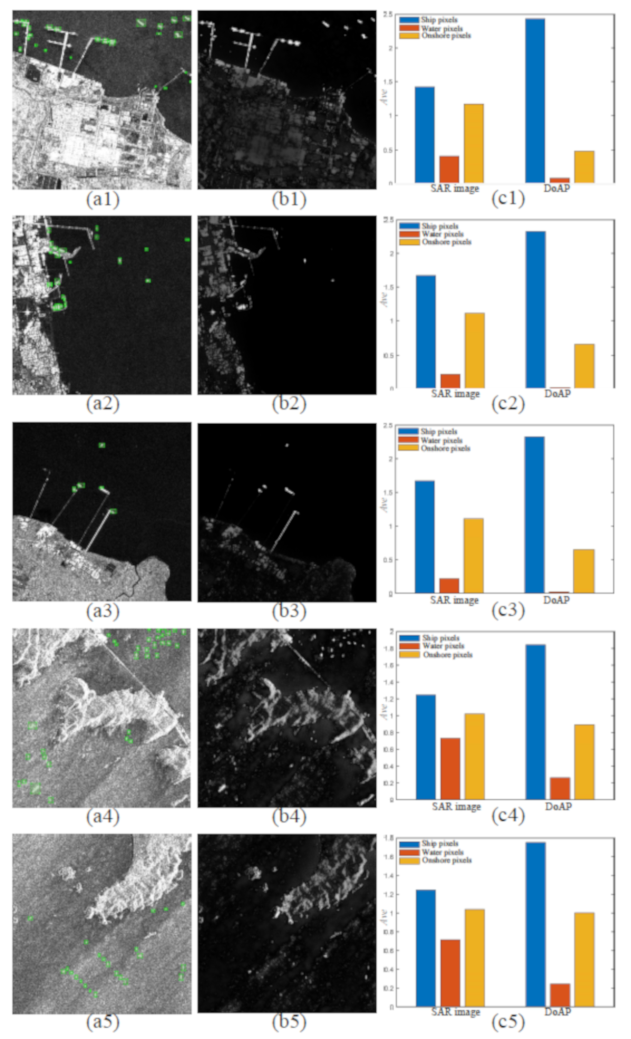
4.2. Final Saliency Enhancement Results

Here, we show the final saliency enhancement results of inshore SAR images with different scenes, as shown in Figure 9. It can be seen from Figure 9(a1,a2) that when there are strong scattering buildings onshore, the contrast between onshore pixels and ship pixels is very low, so it is difficult for inshore ship detection by scattering intensity alone. However, the contrast between onshore pixels and ship pixels can be significantly improved in the final saliency enhancement results, as shown in Figure 9(b1,b2). When the scattering intensity of onshore pixels is low, a large number of onshore pixels can be completely suppressed while enhancing the intensity of ship pixels, as shown in Figure 9(a3,b3). When ship detection is interfered by onshore pixels and complex sea conditions at the same time, a large number of ship signals are covered by background clutters, which easily leads to a large number of false alarms and missed detections, as shown in Figure 9(a4,a5). However, in the final saliency enhancement results obtained by our proposed method, as shown in Figure 9(b4,b5), background clutter is effectively suppressed, whereas ship pixels are preserved. As shown in Figure 9(c1–c5), we can conclude that our proposed DoAP can enhance ship pixels while suppressing water and onshore pixels in SAR images with different scenes.

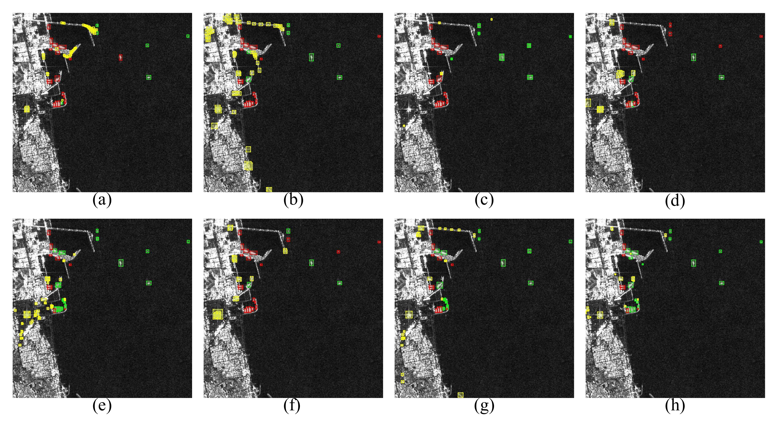
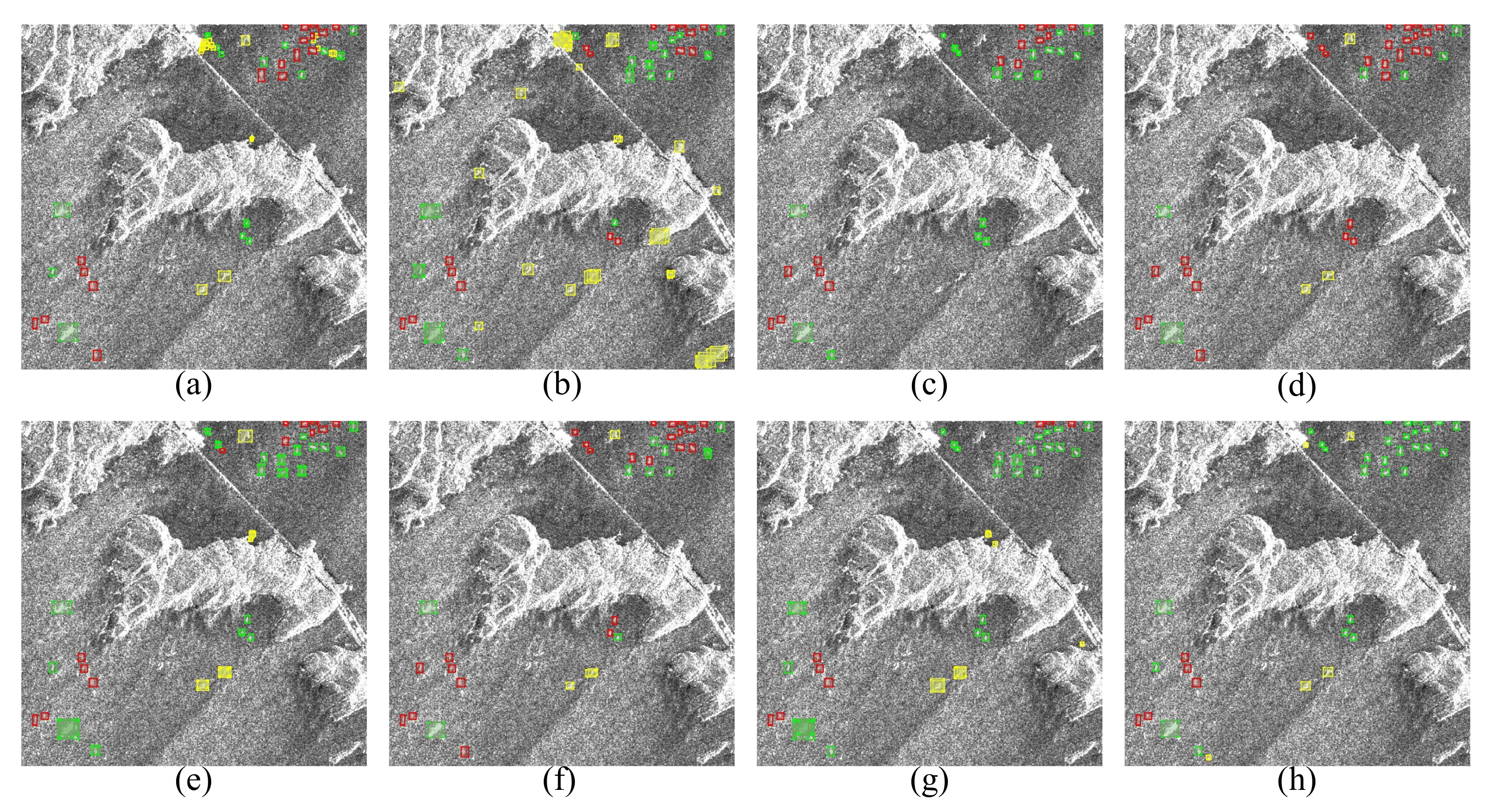
4.3. Comparison with Other Methods

To validate the effectiveness of the proposed method, it is compared with RetinaNet [50], ATSS [51], YOLOv5 [52], Faster R-CNN [53], Double-head R-CNN [54], Cascade R-CNN [29], and Dynamic R-CNN [39]. The detection results of five SAR images with different scenes are shown in Figure 10, Figure 11, Figure 12, Figure 13 and Figure 14. The quantitative comparison results are listed in

Table 2. Quantitative comparison with different detectors on LS-SSDD-v1.0.

Method	Recall (%)	mAP (%)
RetinaNet	79.70	56.80
ATSS	77.30	64.20
YOLOv5	81.00	70.60
Faster R-CNN	72.80	65.30
Double-head R-CNN	78.60	68.40
Cascade R-CNN	74.40	67.20
Dynamic R-CNN	79.10	69.20
Proposed Method	83.90	72.50

.

It can be seen from Figure 10 that the detection results of RetinaNet, ATSS, Faster R-CNN, and Cascade R-CNN all have many missed detections. The detection results of Double-head R-CNN and Dynamic R-CNN both show many onshore false alarms, as shown in Figure 10e,g. The detection results of YOLOv5 have fewer onshore false alarms, but still have some missed detections However, our proposed method is able to detect tiny ships while reducing onshore false alarms.

Due to the negative influence of onshore pixels, a large number of tiny inshore ships are not detected by RetinaNet, ATSS, YOLOv5, Faster R-CNN, and Cascade R-CNN, as shown in Figure 11. Although Double-head R-CNN and Dynamic R-CNN are able to increase the recall of inshore ships, more onshore false alarms are introduced, as shown in Figure 11e,g. Our proposed method further improves the recall of inshore ships and reduces onshore false alarms.

As shown in Figure 12, the detection results of RetinaNet, ATSS, Faster R-CNN, Cascade R-CNN, and Dynamic R-CNN have a lot of onshore false alarms. YOLOv5 and Double-head R-CNN obtain good detection results, but still have few onshore false alarms, as shown in Figure 12e. However, our proposed method obtains the best detection results and the fewest onshore false alarms. The above results indicate that our proposed method can reduce the negative influence of onshore pixels with strong scattering, and obtain the best detection results for tiny ships.

When ships are in an extremely complex background, a large number of ships cannot be detected by RetinaNet, ATSS, YOLOv5, Faster R-CNN, Cascade R-CNN, and Double-head R-CNN, as shown in Figure 13. Dynamic R-CNN obtains good detection results, but still misses some tiny ships, as shown in Figure 13g. However, our method still detects the most ships and gives the fewest false alarms.

As shown in Figure 14, RetinaNet and ATSS produce a lot of false alarms on onshore pixels. We find that many tiny ships in complex sea conditions are not detected by YOLOv5, Faster R-CNN, Double-head R-CNN, and Cascade R-CNN. Dynamic R-CNN improves the recall of inshore ships, and reduces some false alarms, as shown in Figure 14g. Our proposed method further improves the recall of inshore ships by increasing the contrast between ship pixels and water pixels, and reduces the onshore false alarms by increasing the contrast between ship pixels and onshore pixels.

Table 2 gives the quantitative comparison results with different detectors on the LS-SSDD-v1.0 dataset. We can find that RetinaNet obtains the lowest mean average precision (mAP) of 56.80%. Faster R-CNN obtains the lowest recall of 72.80%. The higher recall and lower mAP of RetinaNet and ATSS mean that their detection results have a lot of false alarms. Our proposed method improves the detection performance by 5.30% for recall and 4.10% for mAP, compared to those of Double-head R-CNN; by 9.50% for recall and 5.30% for mAP, comapred to those of Cascade R-CNN; by 4.80% for recall and 3.30% for mAP, compared to those of Dynamic R-CNN; and by 2.90% for recall and 1.90% for mAP, compared to those of YOLOv5.

5. Discussion

Here, we conduct ablation experiments to verify the effectiveness of the saliency enhancement and BLD for different detectors.

Table 3. Ablation experiments on different detectors.

Detector	Saliency Enhancement	BLD	Recall (%)	mAP (%)
RetinaNet	×	×	79.70	56.80
	✓	×	78.80	59.70
	×	✓	76.50	64.10
	✓	✓	78.40	65.20
Faster R-CNN	×	×	72.80	65.30
	✓	×	73.20	66.70
	×	✓	80.80	67.80
	✓	✓	79.50	68.30
Cascade R-CNN	×	×	74.40	67.20
	✓	×	74.70	68.40
	×	✓	81.00	71.20
	✓	✓	81.90	71.40
Dynamic R-CNN	×	×	79.10	69.20
	✓	×	80.40	71.20
	×	✓	83.50	71.80
	✓	✓	83.90	72.50

gives the quantitative results of RetinaNet, Faster R-CNN, Cascade R-CNN, and Dynamic R-CNN. By using saliency enhancement or BLD in RetinaNet, the mAP can be significantly improved, although the recall is slightly reduced. The reason for this is that there are a lot of false alarms in the baseline RetinaNet; saliency enhancement and the BLD are able to reduce false alarms, but inevitably, affects recall. The recall and mAP of Faster R-CNN, Cascade R-CNN, and Dynamic R-CNN can be significantly improved by using saliency enhancement or the BLD. The simultaneous use of saliency enhancement and the BLD can further improve the recall and mAP of Cascade R-CNN and Dynamic R-CNN.

6. Conclusions

In this paper, we propose a saliency enhancement algorithm based on the DoAP and a small-target detector based on the BLD for inshore ship detection in large-scale SAR images. DoAP utilizes a BF to build a anisotropic pyramid, and uses the difference between the finest two scales and the coarsest two scales to generate the saliency map. Extensive experimental results indicate that the DoAP is able to enhance ship pixels and suppress onshore pixels and water pixels. For the reason that ships usually have few pixels in large-scale SAR images, we propose a BLD-based detection framework which replaces IoU with BLD for label assignment and NMS. Finally, the DoAP is embedded into the BLD-based detection framework to detect inshore ships in large-scale SAR images. The experimental results on the LS-SSDD-v1.0 dataset show that our proposed method can effectively detect inshore ships and obtain state-of-the-art detection results. However, the looser bounding box metric would select some low-quality training samples, which decreases the detector performance. In future work, we would evaluate the quality of samples at different scales to decide which samples can be used in model training to obtain more precise detection results based on higher recall rates.

References

1. Renga, A.; Graziano, M.D.; Moccia, A. Segmentation of marine SAR images by sublook analysis and application to sea traffic monitoring. IEEE Trans. Geosci. Remote Sens. 2018, 57, 1463–1477. [Google Scholar] [CrossRef]
2. Cheng, J.; Zhang, F.; Xiang, D.; Yin, Q.; Zhou, Y.; Wang, W. PolSAR Image Land Cover Classification Based on Hierarchical Capsule Network. Remote Sens. 2021, 13, 3132. [Google Scholar] [CrossRef]
3. Hamasaki, T.; Ferro-Famil, L.; Pottier, E.; Sato, M. Applications of polarimetric interferometric ground-based SAR (GB-SAR) system to environment monitoring and disaster prevention. In Proceedings of the European Radar Conference, Paris, France, 3–4 October 2005; pp. 29–32. [Google Scholar]
4. Han, L.; Liu, D.; Guan, D. Ship detection in SAR images by saliency analysis of multiscale superpixels. Remote Sens. Lett. 2022, 13, 708–715. [Google Scholar] [CrossRef]
5. Zhang, T.; Yang, Z.; Gan, H.; Xiang, D.; Zhu, S.; Yang, J. PolSAR ship detection using the joint polarimetric information. IEEE Trans. Geosci. Remote Sens. 2020, 58, 8225–8241. [Google Scholar] [CrossRef]
6. Zhang, T.; Jiang, L.; Xiang, D.; Ban, Y.; Pei, L.; Xiong, H. Ship detection from PolSAR imagery using the ambiguity removal polarimetric notch filter. ISPRS J. Photogramm. Remote Sens. 2019, 157, 41–58. [Google Scholar] [CrossRef]
7. Zhang, T.; Wang, W.; Quan, S.; Yang, H.; Xiong, H.; Zhang, Z.; Yu, W. Region-based Polarimetric Covariance Difference Matrix for PolSAR Ship Detection. IEEE Trans. Geosci. Remote. Sens. 2022, 60, 5222016. [Google Scholar] [CrossRef]
8. Eldhuset, K. An automatic ship and ship wake detection system for spaceborne SAR images in coastal regions. IEEE Trans. Geosci. Remote Sens. 1996, 34, 1010–1019. [Google Scholar]
9. Novak, L.M.; Burl, M.C.; Irving, W. Optimal polarimetric processing for enhanced target detection. IEEE Trans. Aerosp. Electron. Syst. 1993, 29, 234–244. [Google Scholar] [CrossRef]
10. Kuttikkad, S.; Chellappa, R. Non-Gaussian CFAR techniques for target detection in high resolution SAR images. In Proceedings of the 1st International Conference on Image Processing, Austin, TX, USA, 13–16 November 1994; Volume 1, pp. 910–914. [Google Scholar]
11. Tao, D.; Anfinsen, S.N.; Brekke, C. Robust CFAR detector based on truncated statistics in multiple-target situations. IEEE Trans. Geosci. Remote Sens. 2015, 54, 117–134. [Google Scholar] [CrossRef]
12. Zhao, H.; Wang, Q.; Huang, J.; Wu, W.; Yuan, N. Method for inshore ship detection based on feature recognition and adaptive background window. J. Appl. Remote Sens. 2014, 8, 083608. [Google Scholar] [CrossRef]
13. Wang, Q.; Zhu, H.; Wu, W.; Zhao, H.; Yuan, N. Inshore ship detection using high-resolution synthetic aperture radar images based on maximally stable extremal region. J. Appl. Remote Sens. 2015, 9, 095094. [Google Scholar] [CrossRef]
14. Li, A.; Chen, Z. Personalized visual saliency: Individuality affects image perception. IEEE Access 2018, 6, 16099–16109. [Google Scholar] [CrossRef]
15. Zhang, Q.; Wu, Y.; Zhao, W.; Wang, F.; Fan, J.; Li, M. Multiple-scale salient-region detection of SAR image based on Gamma distribution and local intensity variation. IEEE Geosci. Remote Sens. Lett. 2013, 11, 1370–1374. [Google Scholar] [CrossRef]
16. Chen, C.P.; Li, H.; Wei, Y.; Xia, T.; Tang, Y.Y. A local contrast method for small infrared target detection. IEEE Trans. Geosci. Remote Sens. 2013, 52, 574–581. [Google Scholar] [CrossRef]
17. Xie, T.; Zhang, W.; Yang, L.; Wang, Q.; Huang, J.; Yuan, N. Inshore ship detection based on level set method and visual saliency for SAR images. Sensors 2018, 18, 3877. [Google Scholar] [CrossRef] [Green Version]
18. Itti, L.; Koch, C.; Niebur, E. A model of saliency-based visual attention for rapid scene analysis. IEEE Trans. Pattern Anal. Mach. Intell. 1998, 20, 1254–1259. [Google Scholar] [CrossRef] [Green Version]
19. Lai, D.; Xiong, B.; Kuang, G. Weak target detection in SAR images via improved itti visual saliency model. In Proceedings of the 2017 2nd International Conference on Frontiers of Sensors Technologies (ICFST), Shenzhen, China, 14–16 April 2017; pp. 260–264. [Google Scholar]
20. Wang, Z.; Du, L.; Zhang, P.; Li, L.; Wang, F.; Xu, S.; Su, H. Visual attention-based target detection and discrimination for high-resolution SAR images in complex scenes. IEEE Trans. Geosci. Remote Sens. 2017, 56, 1855–1872. [Google Scholar] [CrossRef]
21. Fan, J.; Wu, Y.; Wang, F.; Zhang, Q.; Liao, G.; Li, M. SAR image registration using phase congruency and nonlinear diffusion-based SIFT. IEEE Geosci. Remote Sens. Lett. 2014, 12, 562–566. [Google Scholar]
22. Wang, S.; You, H.; Fu, K. BFSIFT: A novel method to find feature matches for SAR image registration. IEEE Geosci. Remote Sens. Lett. 2011, 9, 649–653. [Google Scholar] [CrossRef]
23. Redmon, J.; Divvala, S.; Girshick, R.; Farhadi, A. You only look once: Unified, real-time object detection. In Proceedings of the IEEE Conference on Computer Vision and Pattern Recognition, Las Vegas, NV, USA, 27–30 June 2016; pp. 779–788. [Google Scholar]
24. Liu, W.; Anguelov, D.; Erhan, D.; Szegedy, C.; Reed, S.; Fu, C.Y.; Berg, A.C. Ssd: Single shot multibox detector. In Proceedings of the European Conference on Computer Vision, Amsterdam, The Netherlands, 11–14 October 2016; pp. 21–37. [Google Scholar]
25. Wang, Y.; Wang, C.; Zhang, H.; Dong, Y.; Wei, S. Automatic ship detection based on RetinaNet using multi-resolution Gaofen-3 imagery. Remote Sens. 2019, 11, 531. [Google Scholar] [CrossRef] [Green Version]
26. Girshick, R.; Donahue, J.; Darrell, T.; Malik, J. Rich feature hierarchies for accurate object detection and semantic segmentation. In Proceedings of the IEEE Conference on Computer Vision and Pattern Recognition, Washington, DC, USA, 23–28 June 2014; pp. 580–587. [Google Scholar]
27. Girshick, R. Fast r-cnn. In Proceedings of the IEEE International Conference on Computer Vision, Washington, DC, USA, 7–13 December 2015; pp. 1440–1448. [Google Scholar]
28. Lin, Z.; Ji, K.; Leng, X.; Kuang, G. Squeeze and excitation rank faster R-CNN for ship detection in SAR images. IEEE Geosci. Remote Sens. Lett. 2018, 16, 751–755. [Google Scholar] [CrossRef]
29. Cai, Z.; Vasconcelos, N. Cascade r-cnn: Delving into high quality object detection. In Proceedings of the IEEE Conference on Computer Vision and Pattern Recognition, Salt Lake City, UT, USA, 18–23 June 2018; pp. 6154–6162. [Google Scholar]
30. Cui, Z.; Li, Q.; Cao, Z.; Liu, N. Dense attention pyramid networks for multi-scale ship detection in SAR images. IEEE Trans. Geosci. Remote Sens. 2019, 57, 8983–8997. [Google Scholar] [CrossRef]
31. Fu, J.; Sun, X.; Wang, Z.; Fu, K. An anchor-free method based on feature balancing and refinement network for multiscale ship detection in SAR images. IEEE Trans. Geosci. Remote Sens. 2020, 59, 1331–1344. [Google Scholar] [CrossRef]
32. Cui, Z.; Wang, X.; Liu, N.; Cao, Z.; Yang, J. Ship detection in large-scale SAR images via spatial shuffle-group enhance attention. IEEE Trans. Geosci. Remote Sens. 2020, 59, 379–391. [Google Scholar] [CrossRef]
33. Du, L.; Li, L.; Wei, D.; Mao, J. Saliency-guided single shot multibox detector for target detection in SAR images. IEEE Trans. Geosci. Remote Sens. 2019, 58, 3366–3376. [Google Scholar] [CrossRef]
34. Yu, J.; Zhou, G.; Zhou, S.; Qin, M. A fast and lightweight detection network for multi-scale SAR ship detection under complex backgrounds. Remote Sens. 2021, 14, 31. [Google Scholar] [CrossRef]
35. Xu, X.; Zhang, X.; Zhang, T.; Shi, J.; Wei, S.; Li, J. On-Board Ship Detection in SAR Images Based on L-YOLO. In Proceedings of the 2022 IEEE Radar Conference (RadarConf22), New York City, NY, USA, 21–25 March 2022; pp. 1–5. [Google Scholar]
36. Xu, X.; Zhang, X.; Zhang, T. Lite-yolov5: A lightweight deep learning detector for on-board ship detection in large-scene sentinel-1 sar images. Remote Sens. 2022, 14, 1018. [Google Scholar] [CrossRef]
37. Wang, J.; Xu, C.; Yang, W.; Yu, L. A Normalized Gaussian Wasserstein Distance for Tiny Object Detection. arXiv 2021, arXiv:2110.13389. [Google Scholar]
38. Tang, J.; Cheng, J.; Xiang, D.; Hu, C. Large-difference-scale Target Detection Using a Revised Bhattacharyya Distance in SAR Images. IEEE Geosci. Remote Sens. Lett. 2022, 19, 4506205. [Google Scholar] [CrossRef]
39. Zhang, H.; Chang, H.; Ma, B.; Wang, N.; Chen, X. Dynamic R-CNN: Towards high quality object detection via dynamic training. In Proceedings of the European Conference on Computer Vision, Glasgow, UK, 23–28 August 2020; pp. 260–275. [Google Scholar]
40. Perona, P.; Malik, J. Scale-space and edge detection using anisotropic diffusion. IEEE Trans. Pattern Anal. Mach. Intell. 1990, 12, 629–639. [Google Scholar] [CrossRef] [Green Version]
41. Alcantarilla, P.F.; Bartoli, A.; Davison, A.J. KAZE features. In Proceedings of the European Conference on Computer Vision, Florence, Italy, 7–13 October 2012; pp. 214–227. [Google Scholar]
42. Niebur, E. Computational architectures for attention. The Attentive Brain; MIT Press: Massachusetts, CA, USA, 1998. [Google Scholar]
43. Liu, S.; Cao, Z.; Li, J. A SVD-based visual attention detection algorithm of SAR image. In Proceedings of the Second International Conference on Communications, Signal Processing and Systems, Tianjin, China, 1–2 September 2014; pp. 479–486. [Google Scholar]
44. Frintrop, S.; Werner, T.; Martin Garcia, G. Traditional saliency reloaded: A good old model in new shape. In Proceedings of the IEEE Conference on Computer Vision and Pattern Recognition, Seattle, WA, USA, 14–19 June 2015; pp. 82–90. [Google Scholar]
45. Wang, J.; Yang, W.; Li, H.C.; Zhang, H.; Xia, G.S. Learning center probability map for detecting objects in aerial images. IEEE Trans. Geosci. Remote Sens. 2020, 59, 4307–4323. [Google Scholar] [CrossRef]
46. Joyce, J.M. Kullback-leibler divergence. In International Encyclopedia of Statistical Science; Springer: New York, NY, USA, 2011; pp. 720–722. [Google Scholar]
47. Menéndez, M.; Pardo, J.; Pardo, L.; Pardo, M. The jensen-shannon divergence. J. Frankl. Inst. 1997, 334, 307–318. [Google Scholar] [CrossRef]
48. Schweppe, F.C. On the Bhattacharyya distance and the divergence between Gaussian processes. Inf. Control 1967, 11, 373–395. [Google Scholar] [CrossRef] [Green Version]
49. Zhang, T.; Zhang, X.; Ke, X.; Zhan, X.; Shi, J.; Wei, S.; Pan, D.; Li, J.; Su, H.; Zhou, Y.; et al. LS-SSDD-v1. 0: A deep learning dataset dedicated to small ship detection from large-scale Sentinel-1 SAR images. Remote Sens. 2020, 12, 2997. [Google Scholar] [CrossRef]
50. Lin, T.Y.; Goyal, P.; Girshick, R.; He, K.; Dollár, P. Focal loss for dense object detection. In Proceedings of the IEEE International Conference on Computer Vision, Venice, Italy, 22–29 October 2017; pp. 2980–2988. [Google Scholar]
51. Zhang, S.; Chi, C.; Yao, Y.; Lei, Z.; Li, S.Z. Bridging the gap between anchor-based and anchor-free detection via adaptive training sample selection. In Proceedings of the IEEE/CVF Conference on Computer Vision and Pattern Recognition, Seattle, WA, USA, 13–19 June 2020; pp. 9759–9768. [Google Scholar]
52. Ultralytics. YOLOv5. 2020. Available online: https://github.com/ultralytics/yolov5 (accessed on 18 May 2020).
53. Ren, S.; He, K.; Girshick, R.; Sun, J. Faster r-cnn: Towards real-time object detection with region proposal networks. In Proceedings of the Advances in Neural Information Processing Systems 28 (NIPS 2015), Montreal, QC, Canada, 7–12 December 2015. [Google Scholar]
54. Wu, Y.; Chen, Y.; Yuan, L.; Liu, Z.; Wang, L.; Li, H.; Fu, Y. Rethinking classification and localization for object detection. In Proceedings of the IEEE/CVF Conference on Computer Vision and Pattern Recognition, Seattle, WA, USA, 13–19 June 2020; pp. 10186–10195. [Google Scholar]
Figure 1. A difficult case of inshore ship detection in an SAR image. (a) SAR image acquired by TreeaSAR-X with 3 m resolution. (b) The mesh map of the SAR image intensity. The inshore ships and harbor facilities are marked in blue and red dotted circles, respectively. This indicates that inshore ships are difficult to separate from onshore pixels through scattering intensity alone.
Remotesensing 14 02832 g001
Figure 2. IoU of a large ship and a small ship. (a) Large ship detection. (b) SAR image. (c) Small ship detection. A is the ground truth bounding box, B and C are the proposal bounding boxes with one- and three-pixel location deviations, respectively.
Remotesensing 14 02832 g002
Figure 3. Overall architecture of the proposed method.
Remotesensing 14 02832 g003
Figure 4. Schematic diagram of the DoAP. Numbers 1–6 denote different scales of the image pyramid.
Remotesensing 14 02832 g004
Figure 5. Schematic diagram of the bilinear interpolation algorithm.
Remotesensing 14 02832 g005
Figure 6. Saliency enhancement results with different methods. (a) SAR image. (b) Ground truth of ships. (c) The mesh map of the SAR image intensity. (d) Saliency map obtained by DoG. (e) Final saliency enhancement result obtained by DoG. (f) The mesh map of (e). (g) Saliency map obtained by Itti. (h) Final saliency enhancement result obtained by Itti. (i) The mesh map of (h). (j) Saliency map obtained by DoAP. (k) Final saliency enhancement result obtained by DoAP. (l) The mesh map of (k).
Remotesensing 14 02832 g006
Figure 7. The contrast of ship pixels, water pixels, and onshore pixels.
Remotesensing 14 02832 g007
Figure 8. A comparison of (a) and (e) IoU curves, (b) and (f) NWD curves, (c) and (g) NBD curves, and (d) and (h) NBLD curves. (a)–(d) are with s i z e A = s i z e B . (e)–(h) are with s i z e A = 4 × s i z e B . The abscissa value represents the location deviation between the center points of bounding boxes A and B.
Remotesensing 14 02832 g008
Figure 9. Results of final saliency enhancement. (a1)–(a5) Ground truth maps. (b1)–(b5) Final saliency enhancement results obtained by the DoAP. (c1)–(c5) The contrast results of ship pixels, water pixels, and onshore pixels.
Remotesensing 14 02832 g009
Figure 10. Visualization of detection results with different detectors in scene 1. (a) RetinaNet. (b) ATSS. (c) YOLOv5. (d) Faster R-CNN. (e) Double-head R-CNN. (f) Cascade R-CNN. (g) Dynamic R-CNN. (h) The proposed method.
Remotesensing 14 02832 g010
Figure 11. Visualization of detection results with different detectors in scene 2. (a) RetinaNet. (b) ATSS. (c) YOLOv5. (d) Faster R-CNN. (e) Double-head R-CNN. (f) Cascade R-CNN. (g) Dynamic R-CNN. (h) The proposed method.
Remotesensing 14 02832 g011
Figure 12. Visualization of detection results with different detectors in scene 3. (a) RetinaNet. (b) ATSS. (c) YOLOv5. (d) Faster R-CNN. (e) Double-head R-CNN. (f) Cascade R-CNN. (g) Dynamic R-CNN. (h) The proposed method.
Remotesensing 14 02832 g012
Figure 13. Visualization of detection results with different detectors in scene 4. (a) RetinaNet. (b) ATSS. (c) YOLOv5. (d) Faster R-CNN. (e) Double-head R-CNN. (f) Cascade R-CNN. (g) Dynamic R-CNN. (h) The proposed method.
Remotesensing 14 02832 g013
Figure 14. Visualization of detection results with different detectors in scene 5. (a) RetinaNet. (b) ATSS. (c) YOLOv5. (d) Faster R-CNN. (e) Double-head R-CNN. (f) Cascade R-CNN. (g) Dynamic R-CNN. (h) The proposed method.
Remotesensing 14 02832 g014