
Comparison of Pond Depth and Ice Thickness Retrieval Algorithms for Summer Arctic Sea Ice


Abstract
:
1. Introduction
2. Methods and Data
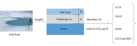
2.1. Methods
2.1.1. Algorithm of Lu18
2.1.2. Algorithm of Malinka18
2.1.3. Algorithm of König20
2.1.4. Algorithm of Legleiter14 and Zhang21
2.2. Data
3. Results
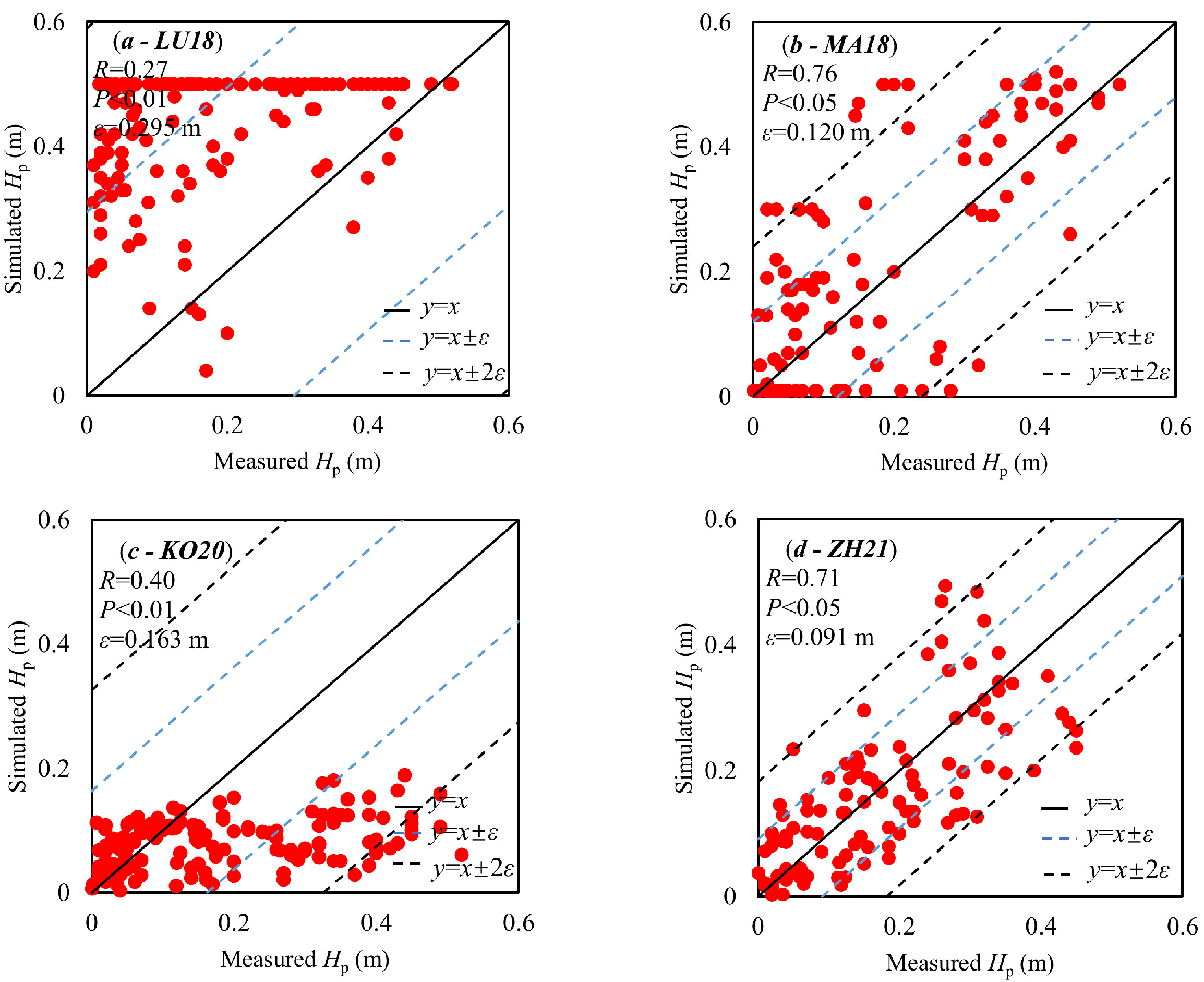
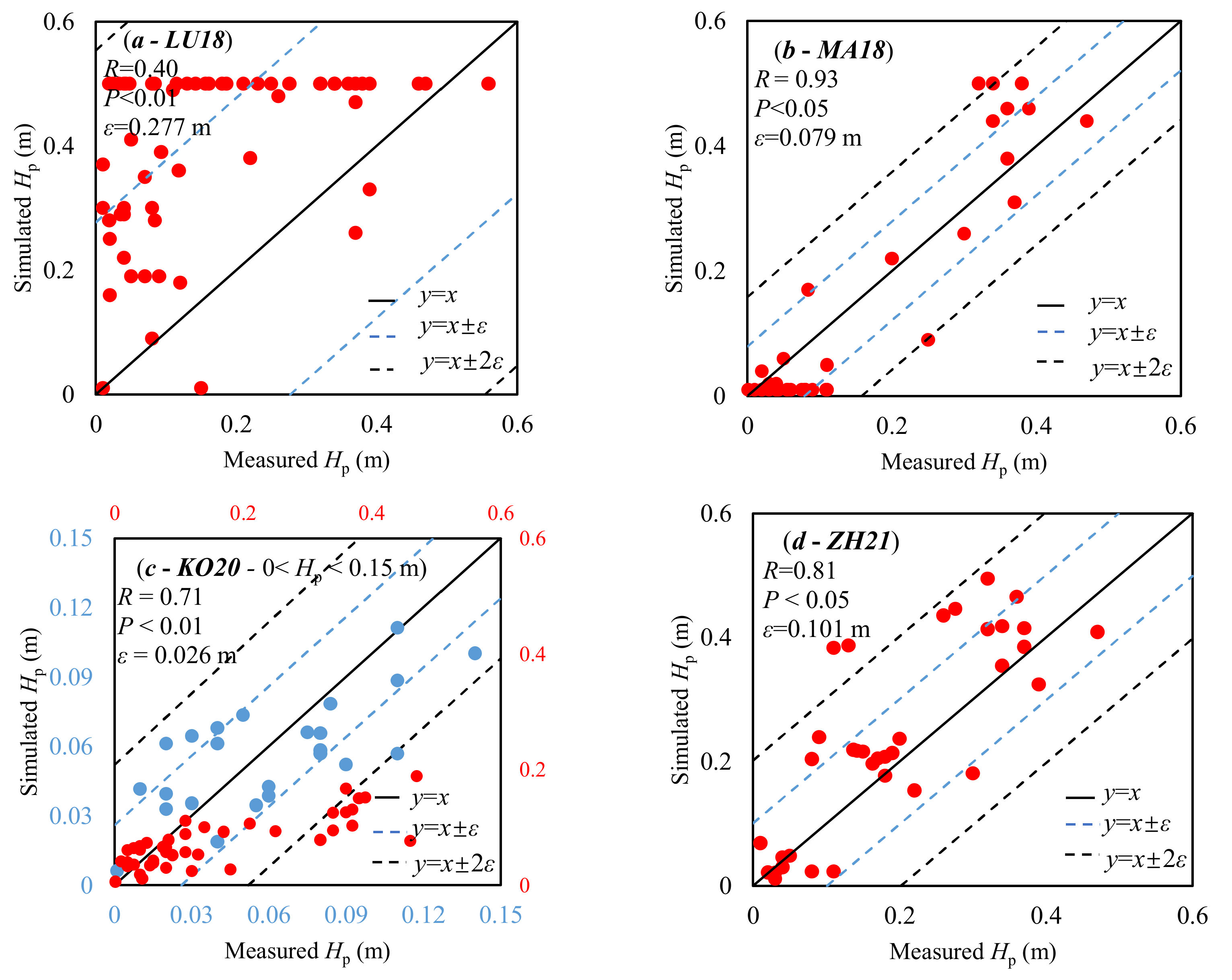
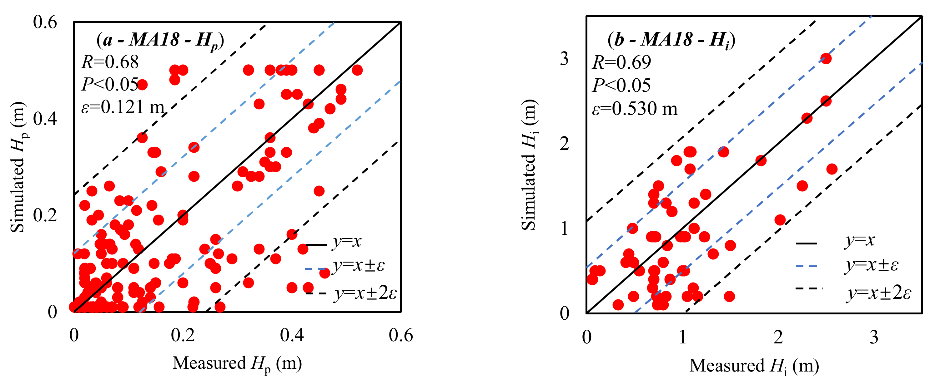
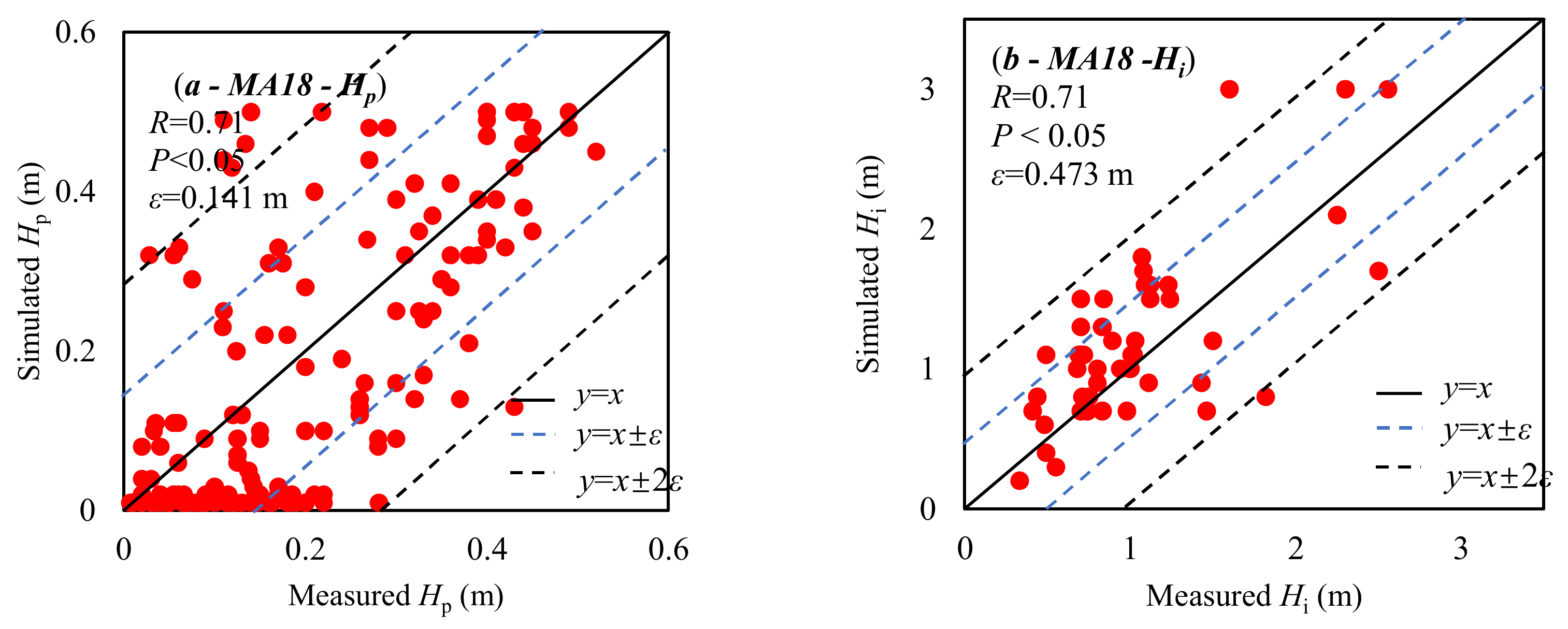
3.1. Retrievals of Pond Depth
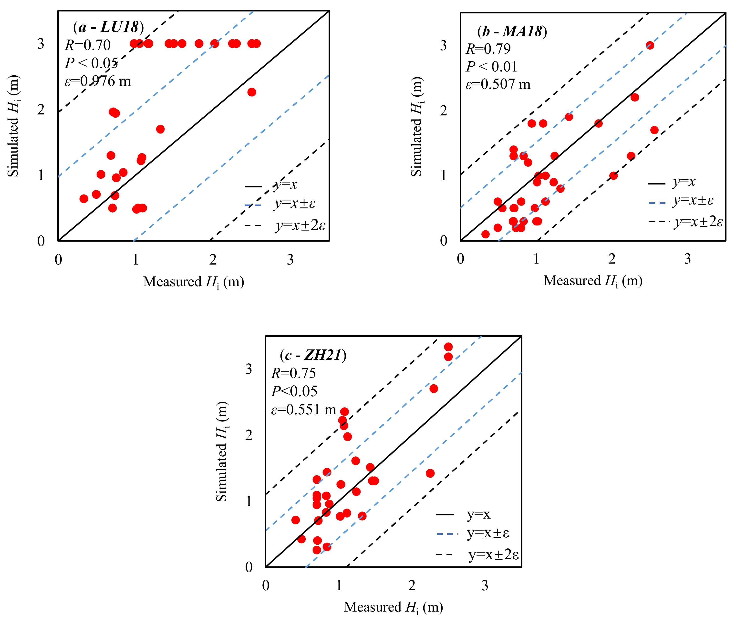
3.2. Retrievals of Underlying Ice Thickness
4. Discussions on Application
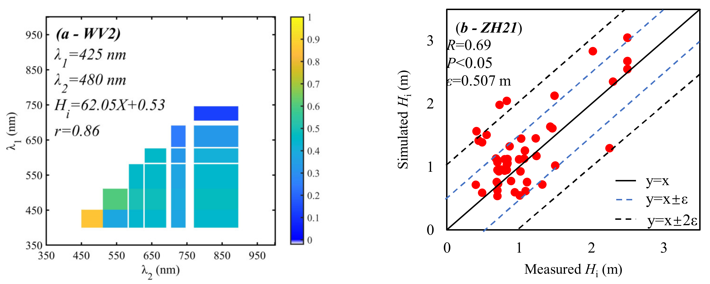
4.1. The Application for the Satellite Optical Data
4.2. The Application for In Situ Optical Data
5. Conclusions
Author Contributions
Funding
Data Availability Statement
Acknowledgments
Conflicts of Interest
References
- Katlein, C.; Arndt, S.; Nicolaus, M.; Perovich, D.K.; Jakuba, M.V.; Suman, S.; Elliott, S.; Whitcomb, L.L.; McFarland, C.J.; Gerdes, R.; et al. Influence of ice thickness and surface properties on light transmission through Arctic sea ice. J. Geophys. Res. Ocean. 2015, 120, 5932–5944. [Google Scholar] [CrossRef] [PubMed]
- Nicolaus, M.; Arndt, S.; Katlein, C.; Maslanik, J.; Hendricks, S. Changes in Arctic sea ice result in increasing light transmittance and absorption. Geophys. Res. Lett. 2012, 40, 2699–2700. [Google Scholar] [CrossRef] [Green Version]
- Notz, D.; Worster, M.G. Desalination processes of sea ice revisited. J. Geophys. Res. Ocean. 2009, 114, C05006. [Google Scholar] [CrossRef] [Green Version]
- Wang, M.; Su, J.; Landy, J.; Leppäranta, M.; Guan, L. A new algorithm for sea ice melt pond fraction estimation from high-resolution optical satellite imagery. J. Geophys. Res. Ocean. 2021, 125, e2019JC015716. [Google Scholar] [CrossRef]
- Li, L.; Ke, C.; Xie, H.; Lei, R.; Tao, A. Aerial observations of sea ice and melt ponds near the North Pole during CHINARE2010. Acta Oceanol. Sin. 2017, 36, 64–72. [Google Scholar] [CrossRef]
- Perovich, D.K.; Tucker, W.B., III; Ligett, K.A. Aerial observation of the evolution of ice surface conditions during summer. J. Geophys. Res. 2002, 107, SHE-24. [Google Scholar] [CrossRef]
- Lu, P.; Leppäranta, M.; Cheng, B.; Li, Z. Influence of melt-pond depth and ice thickness on Arctic sea-ice albedo and light transmittance. Cold Reg. Sci. Technol. 2016, 124, 1–10. [Google Scholar] [CrossRef]
- Flocco, D.; Feltham, D.L.; Bailey, E.; Schroeder, D. The refreezing of melt ponds on Arctic sea ice. J. Geophys. Res. Ocean. 2015, 120, 647–659. [Google Scholar] [CrossRef] [Green Version]
- Fetterer, F.; Untersteiner, N. Observations of melt ponds on Arctic sea ice. J. Geophys. Res. 1998, 103, 821–835. [Google Scholar] [CrossRef]
- Lu, P.; Cheng, B.; Leppäranta, M.; Li, Z. Partitioning of solar radiation in Arctic sea ice during melt season. Oceanologia 2018, 60, 464–477. [Google Scholar] [CrossRef]
- Holland, M.M.; Bitz, C.M.; Tremblay, B. Future abrupt reductions in the summer Arctic sea ice. Geophys. Res. Lett. 2006, 33, L23503. [Google Scholar] [CrossRef] [Green Version]
- Ji, Q. Study on Spatial-Temporal Change of Arctic Sea Ice Thickness Based on Satellite Altimetry. Ph.D. Thesis, Wuhan University, Wuhan, China, 2015. [Google Scholar]
- Kwok, R.; Cunningham, G.F. ICESat over Arctic sea ice: Estimation of snow depth and ice thickness. J. Geophys. Res. Ocean. 2008, 113, C08010. [Google Scholar] [CrossRef]
- Ji, Q.; Pang, X.; Zhao, X.; Cheng, Z. Comparison of Sea Ice Thickness Retrieval Algorithms from CryoSat-2 Satellite Altimeter Data. Geomat. Inf. Sci. Wuhan Univ. 2015, 40, 1467–1472. [Google Scholar]
- Farrel, S.L.; Duncan, K.; Buckley, E.M.; Richter-Menge, J.; Li, R. Mapping sea ice surface topography in high fidelity with ICESst-2. Geophys. Res. Lett. 2020, 47, e2020GL090708. [Google Scholar]
- Perovich, D.K.; Grenfell, T.C.; Richter-Menge, J.A.; Light, B.; Tucker, W.B., III; Eicken, H. Thin and thinner: Sea ice mass balance measurement during SHEBA. J. Geophys. Res. Ocean. 2003, 108, C38050. [Google Scholar] [CrossRef]
- Legleiter, C.J.; Tedesco, M.; Smith, L.C.; Behar, A.E.; Overstreet, B.T. Mapping the bathymetry of supraglacial lakes and streams on the Greenland ice sheet using field measurements and high-resolution satellite images. Cryosphere 2014, 8, 215–228. [Google Scholar] [CrossRef] [Green Version]
- Malinka, A.; Zege, E.; Istomina, L.; Heygster, G.; Spreen, G.; Perovich, D.; Polashenski, C. Reflective properties of melt ponds on sea ice. Cryosphere 2018, 12, 1921–1937. [Google Scholar] [CrossRef] [Green Version]
- Lu, P.; Leppäranta, M.; Cheng, B.; Li, Z.; Istomina, L.; Heygster, G. The color of melt ponds on Arctic sea ice. Cryosphere 2018, 12, 1331–1345. [Google Scholar] [CrossRef] [Green Version]
- König, M.; Oppelt, N. A linear model to derive melt pond depth on Arctic sea ice from hyperspectral data. Cryosphere 2020, 14, 2567–2579. [Google Scholar] [CrossRef]
- Zhang, H.; Yu, M.; Lu, P.; Zhou, J.; Li, Z. Retrievals of Arctic sea ice melt pond depth and underlying ice thickness using optical data. Adv. Polar Sci. 2021, 32, 105–117. [Google Scholar]
- Briegleb, B.P.; Light, B. A Delta-Eddington Multiple Scattering Parameterization for Solar Radiation in the Sea Ice Component of the Community Climate System Model (NO. NCAR/TN-472+STR); University Corporation for Atmospheric Research: Boulder, CO, USA, 2007. [Google Scholar]
- Perovich, D.K. The optical properties of sea ice. In US Army Cold Regions Research and Engineering Laboratory (CRREL) Report 96-1; Cold Regions Research and Engineering Laboratory: Hanover, NH, USA, 1996; Available online: http://www.dtic.mil/cgi-bin/GetTRDoc?AD=ADA310586 (accessed on 11 July 2021).
- Grenfell, T.C.; Perovich, D.K. Incident spectral irradiance in the Arctic Basin during the summer and fall. J. Geophys. Res. Atmos. 2008, 113, D12117. [Google Scholar] [CrossRef]
- Warren, S.G.; Brandt, R.E. Optical constants of ice from the ultraviolet to the microwave: A revised compilation. J. Geophys. Res. Atmos. 2008, 113, D14220. [Google Scholar] [CrossRef]
- Daimon, M.; Masumura, A. Measurement of the refractive index of distilled water from the near-infrared region to the ultraviolet region. Appl. Opt. 2007, 46, 3811–3820. [Google Scholar] [CrossRef] [PubMed]
- Kedenburg, S.; Vieweg, M.; Gissibl, T.; Giessen, H. Linear refractive index and absorption measurements of nonlinear optical liquids in the visible and near-infrared spectral region. Opt. Mater. Express 2012, 2, 1588–1611. [Google Scholar] [CrossRef]
- Malinka, A. Light scattering in porous materials: Geometrical optics and stereological approach. J. Quant. Spectrosc. Radiat. Transf. 2014, 141, 10–23. [Google Scholar] [CrossRef]
- Segeistein, D.J. The Complex Refractive Index of Water. Master’s Thesis, University of Missouri, Columbia, MO, USA, 1981. Available online: http://mospace.umsystem.edu/xmlui/handle/10355/11599 (accessed on 21 August 2021).
- Kopelevich, O.V. Low-parametric model of seawater optical properties. In Ocean Optics I: Physical Ocean Optics; Monin, A.S., Ed.; Nauka: Moscow, Russia, 1983; pp. 208–234. [Google Scholar]
- Morassutti, M.P.; Ledrew, E.F. Albedo and depth of melt ponds on sea-ice. Int. J. Climatol. 1996, 16, 817–838. [Google Scholar] [CrossRef]
- Istomina, L.; Nicolaus, M.; Perovich, D.K. Surface Spectral Albedo Complementary to ROV Transmittance Measurements at 6 Ice Stations during POLARSTERN Cruise ARK-XXⅦ/3 (IceArc) in 2012. PANGAEA 2016. [Google Scholar] [CrossRef]
- Malinka, A.; Zege, E.; Heygster, G.; Istomina, L. Reflective properties of white sea ice and snow. Cryosphere 2016, 10, 2541–2557. [Google Scholar] [CrossRef] [Green Version]
- Tomasi, C.; Vitale, A.; Lupi, A.; Carmine, C.D.; Campanelli, M.C.; Herber, A.; Treffeisen, R.; Stone, R.S.; Andrews, E.; Sharma, S.; et al. Aerosols in polar regions: A historical overview based on optical depth and in situ observations. J. Geophys. Res. Atmos. 2007, 112, D16205. [Google Scholar] [CrossRef]
- Perovich, D.K. Observations of the polarization of light reflected from sea ice. J. Geophys. Res. Ocean. 1998, 103, 5563–5575. [Google Scholar] [CrossRef]
- Perovich, D.K.; Andreas, E.L.; Curry, J.A.; Eiken, H.; Fairall, C.W.; Grenfell, T.C.; Guest, P.S.; Intrieri, J.; Kadko, D.; Lindsay, R.W.; et al. Year on ice given climate insights. Eos Trans. Am. Geophys. Union 1999, 80, 485–486. [Google Scholar] [CrossRef]
- Perovich, D.K.; Grenfell, T.C.; Light, B.; Hobbs, P.V. Seasonal evolution of the albedo of multiyear Arctic sea ice. J. Geophys. Res. Oceans. 2002, 107, SHE-20. [Google Scholar] [CrossRef]
- Polashenski, C.; Perovich, D.; Courville, Z. The mechanisms of sea ice melt pond formation and evolution. J. Geophys. Res. Ocean. 2012, 117, C01001. [Google Scholar] [CrossRef]
- Light, B.; Perovich, D.K.; Webster, M.A.; Polashenski, C.P.; Dadic, R. Optical properties of melting first-year Arctic sea ice. J. Geophys. Res. Ocean. 2015, 120, 7657–7675. [Google Scholar] [CrossRef]
- Wang, Q.; Li, Z.; Lu, P.; Lei, R.; Cheng, B. 2014 summer Arctic sea ice thickness and concentration from shipborne observations. Int. J. Digit. Earth 2019, 12, 931–947. [Google Scholar] [CrossRef]
- Cao, X.; Lu, P.; Lei, R.; Wang, Q.; Li, Z. Physical and optical characteristics of sea ice in the Pacific Arctic Sector during the summer of 2018. Acta Oceanol. Sin. 2020, 39, 25–37. [Google Scholar] [CrossRef]
- Lu, P.; Cao, X.; Wang, Q.; Leppäranta, M.; Cheng, B.; Li, Z. Impact of a surface ice lid on the optical properties of melt ponds. J. Geophys. Res. Ocean. 2018, 123, 8313–8328. [Google Scholar] [CrossRef]
- Makshtas, A.P.; Podgorny, I.A. Calculation of melt pond albedos on arctic sea ice. Polar Res. 1996, 15, 43–52. [Google Scholar] [CrossRef]
- Legleiter, C.J.; Robert, D.A.; Lawrence, R.L. Spectrally based remote sensing of river bathymetry. Earth Surf. Process. Landf. 2009, 34, 1039–1059. [Google Scholar] [CrossRef]
- Webster, M.A.; Rigor, I.G.; Perovich, D.K.; Richter-Menge, J.A.; Polashenski, C.M.; Light, B. Seasonal evolution of melt ponds on Arctic sea ice. J. Geophys. Res. Oceans. 2015, 120, 5968–5982. [Google Scholar] [CrossRef]
- Taskjelle, T.; Hudson, S.R.; Granskog, M.A.; Hamre, B. Modelling radiative transfer through ponded first-year Arctic sea ice with a plane-parallel model. Cryosphere 2017, 11, 2137–2148. [Google Scholar] [CrossRef] [Green Version]
- Lindsay, R.; Schweiger, A. Arctic sea ice thickness loss determined using subsurface, aircraft, and satellite observations. Cryosphere 2015, 9, 269–283. [Google Scholar] [CrossRef] [Green Version]
- Zege, E.; Malinka, A.; Katsev, I.; Prikhach, A.; Heygster, G.; Istomina, L.; Birnbaum, G.; Schwarz, P. Algorithm to retrieve the melt pond fraction and the spectral albedo of Arctic summer ice from satellite optical data. Remote Sens. Environ. 2015, 163, 153–164. [Google Scholar] [CrossRef] [Green Version]


| Source | Location | Measure Time | Size | Hp | Hi | Measured Data | Albedo Wavelength | Sky Condition |
|---|---|---|---|---|---|---|---|---|
| Perovich [35] | Near 71°N, 156°W | 1995.6.9 | - | 0.06 m | 1.6 m | Albedo and color | 400–1000 nm | Clear sky |
| Perovich et al. [36] | 75°N, 142°W to 80°N, 162°W | 1998.6–1998.8 | <35 m | 0–0.5 m | - | Albedo | 399–1000 nm | Clear and overcast sky |
| Perovich et al. [37] Malinka et al. [18] | 75°N, 142°W to 80°N, 162°W | 1998.6–1998.8 | - | 0–0.5 m | 0–1.2 m | Albedo | 400–1000 nm | Overcast sky |
| Polashenski et al. [38] | Near 71°N, 156°W | 2008.6 and 2009.6 | <20 m | 0–0.3 m | - | Albedo and color | 350–1300 nm | Clear and overcast sky |
| Light et al. [39] | 67°N, 150°W to 75°N, 175°W | 2010.6 and 2011.7 | <20 m | 0–0.37 m | 0.49–1.5 m | Albedo | 350–1300 nm | Clear and overcast sky |
| Istomina et al. [32] | 84°N, 31°E to 82°N, 129°E | 2012.8 | - | 0–0.5 m | 0.4–3 m | Albedo and color | 350–1300 nm | Clear and overcast sky |
| Wang et al. [40] | 76°N, 167°W to 83°N, 180°W | 2016.8 | - | 0–0.3 m | 0.5–1 m | Albedo and color | 350–950 nm | Overcast sky |
| Cao et al. [41] | 79°N, 156°W to 85°N, 170°W | 2018.8 | - | 0–0.3 m | 1–1.5 m | Albedo and color | 350–920 nm | Overcast sky |
| Algorithm | Input Parameters | Output Parameters | Overcast Sky Accuracies | Clear Sky Accuracies | Application | Illumination Condition | Instrument Setups |
|---|---|---|---|---|---|---|---|
| LU18 | Melt pond color (RGB) | Hp and Hi | Hp: R = 0.27 ε = 0.295 m Hi: R = 0.70 ε = 0.976 m | Hp: R = 0.40 ε = 0.277 m | In situ measure of optical data | Clear and overcast sky conditions | Digital camera |
| MA18 | Melt pond surface spectral albedo | Hp and Hi | Hp: R = 0.76 ε = 0.120 m Hi: R = 0.79 ε = 0.507 m | Hp: R = 0.93 ε = 0.079 m | Satellite optical data In situ measure of optical data | Clear and overcast sky conditions | Spectrometers |
| KO20 | The slope of the log-scaled albedo at 710 nm and the solar zenith angle | Hp | Hp: R = 0.40 ε = 0.163 m | Hp: R = 0.71 (0 < Hp < 0.15 m) ε = 0.026 m | In situ measure of optical data | Clear sky conditions | Spectrometers |
| ZH21 | Melt pond surface spectral albedo | Hp and Hi | Hp: R = 0.71 ε = 0.091 m Hi: R = 0.75 ε = 0.551 m | Hp: R = 0.81 ε = 0.101 m | Satellite optical data In situ measure of optical data | Clear and overcast sky conditions | Spectrometers |
Publisher’s Note: MDPI stays neutral with regard to jurisdictional claims in published maps and institutional affiliations. |
© 2022 by the authors. Licensee MDPI, Basel, Switzerland. This article is an open access article distributed under the terms and conditions of the Creative Commons Attribution (CC BY) license (https://creativecommons.org/licenses/by/4.0/).
Share and Cite
Zhang, H.; Lu, P.; Yu, M.; Zhou, J.; Wang, Q.; Li, Z.; Zhang, L. Comparison of Pond Depth and Ice Thickness Retrieval Algorithms for Summer Arctic Sea Ice. Remote Sens. 2022, 14, 2831. https://doi.org/10.3390/rs14122831
Zhang H, Lu P, Yu M, Zhou J, Wang Q, Li Z, Zhang L. Comparison of Pond Depth and Ice Thickness Retrieval Algorithms for Summer Arctic Sea Ice. Remote Sensing. 2022; 14(12):2831. https://doi.org/10.3390/rs14122831
Chicago/Turabian StyleZhang, Hang, Peng Lu, Miao Yu, Jiaru Zhou, Qingkai Wang, Zhijun Li, and Limin Zhang. 2022. "Comparison of Pond Depth and Ice Thickness Retrieval Algorithms for Summer Arctic Sea Ice" Remote Sensing 14, no. 12: 2831. https://doi.org/10.3390/rs14122831
APA StyleZhang, H., Lu, P., Yu, M., Zhou, J., Wang, Q., Li, Z., & Zhang, L. (2022). Comparison of Pond Depth and Ice Thickness Retrieval Algorithms for Summer Arctic Sea Ice. Remote Sensing, 14(12), 2831. https://doi.org/10.3390/rs14122831