
Generalized Additive Model Reveals Nonlinear Trade-Offs/Synergies between Relationships of Ecosystem Services for Mountainous Areas of Southwest China


Abstract
:
1. Introduction
2. Materials and Methods
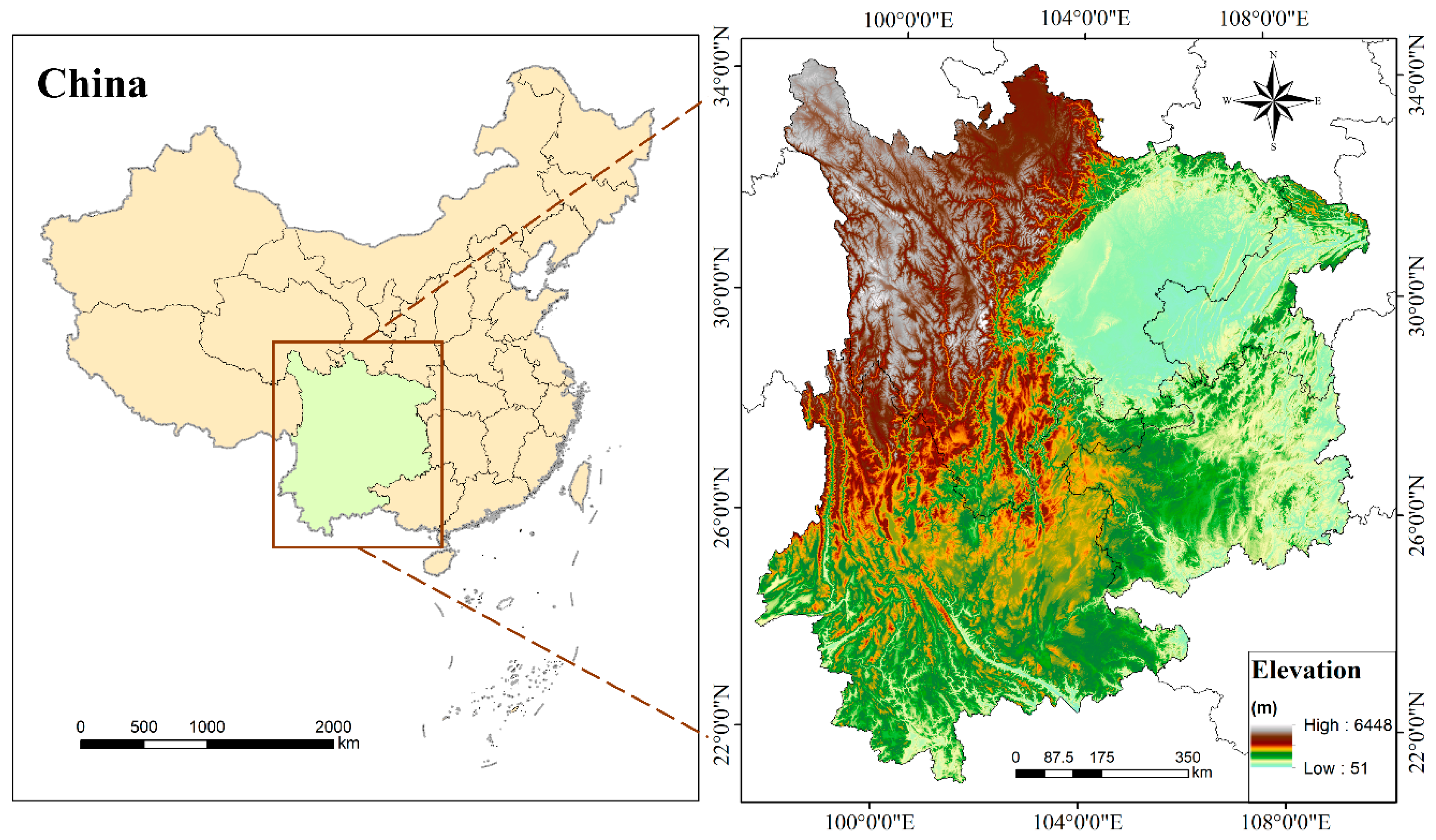
2.1. Study Area
2.2. Sources of Data
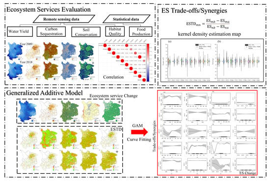
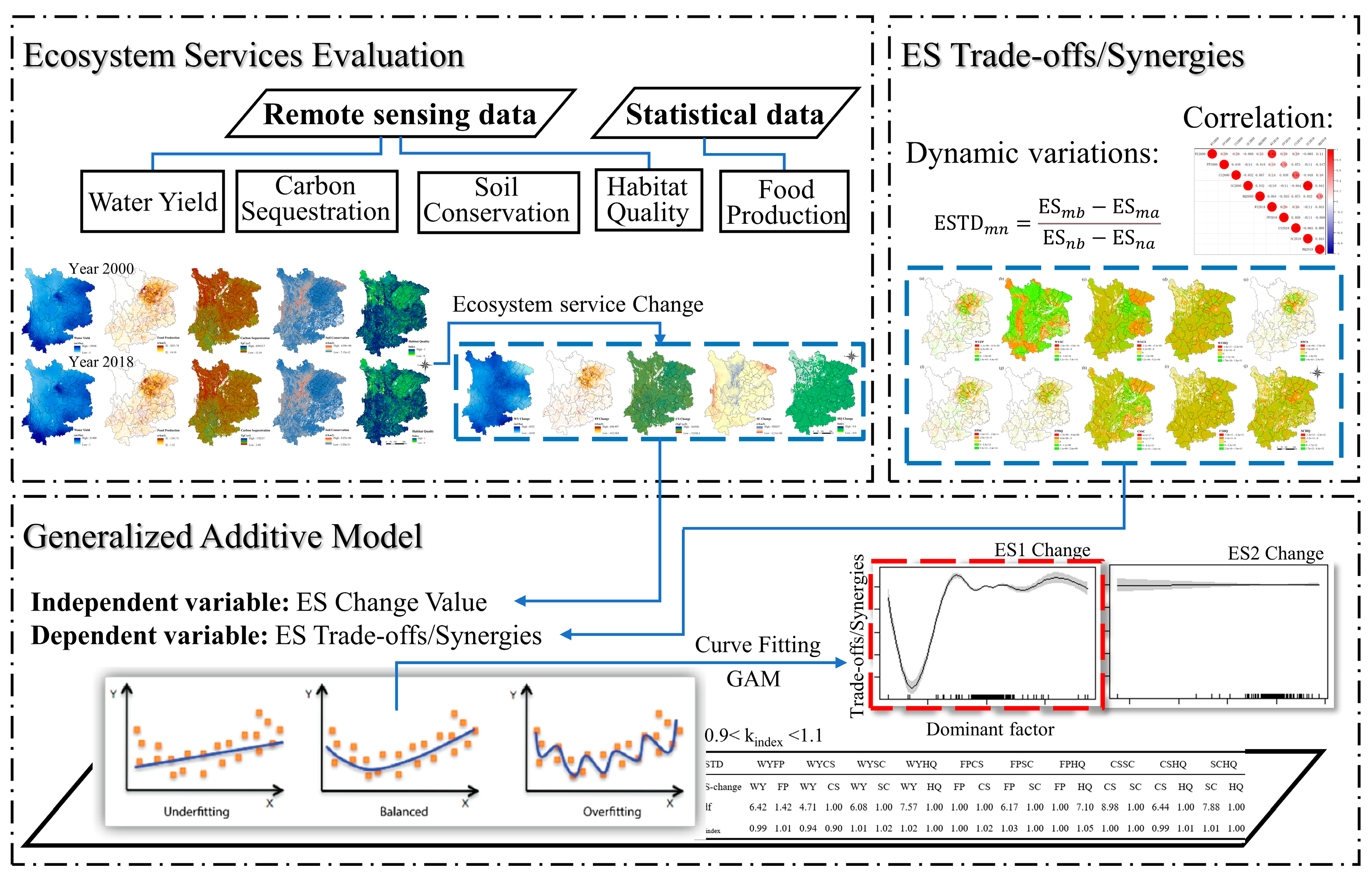
2.3. Methodology
2.3.1. ES Evaluation
2.3.2. Trade-Off/Synergy Calculations
2.3.3. Fitting the Response Curve among ESs
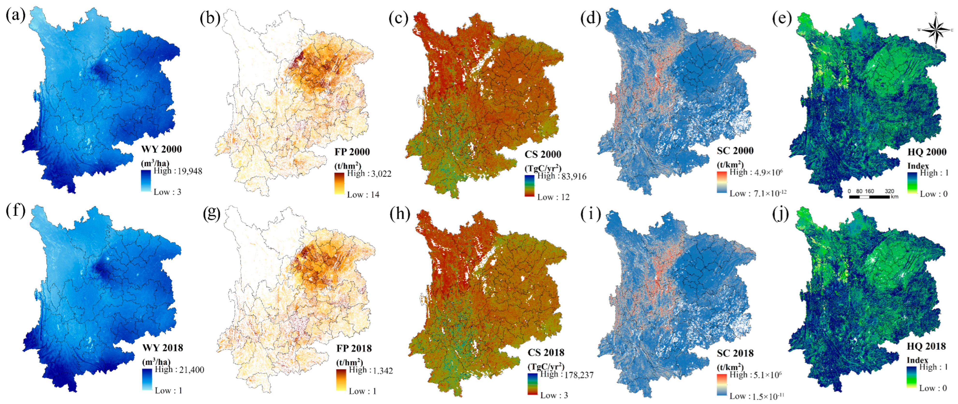
3. Results
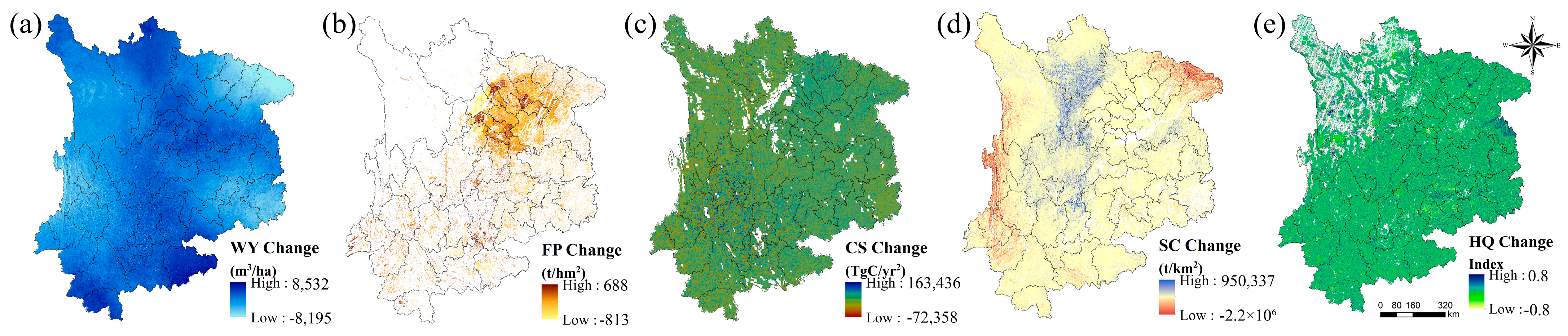
3.1. ESs
3.2. ESs Trade-Off/Synergy
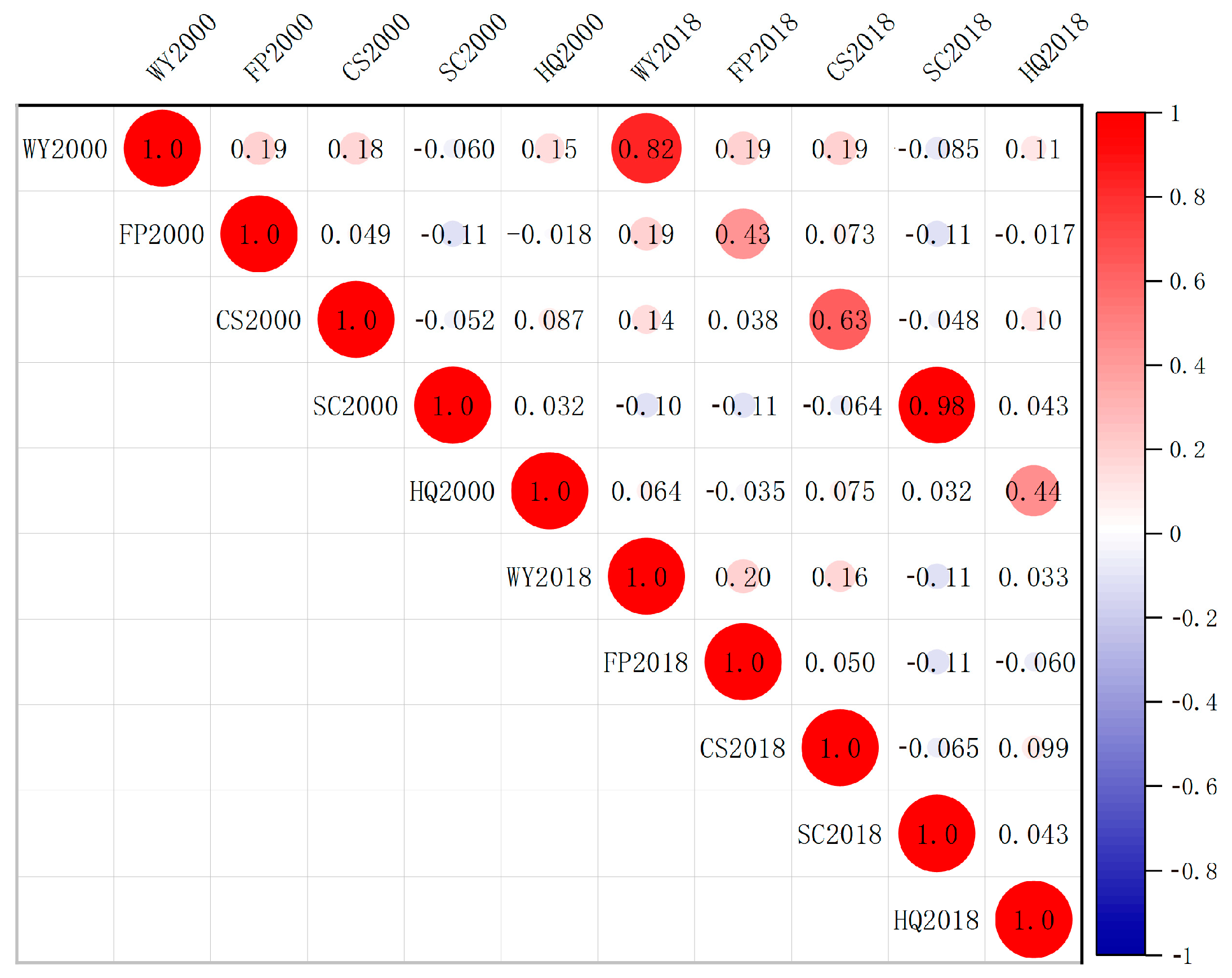
3.2.1. ESs Correlation
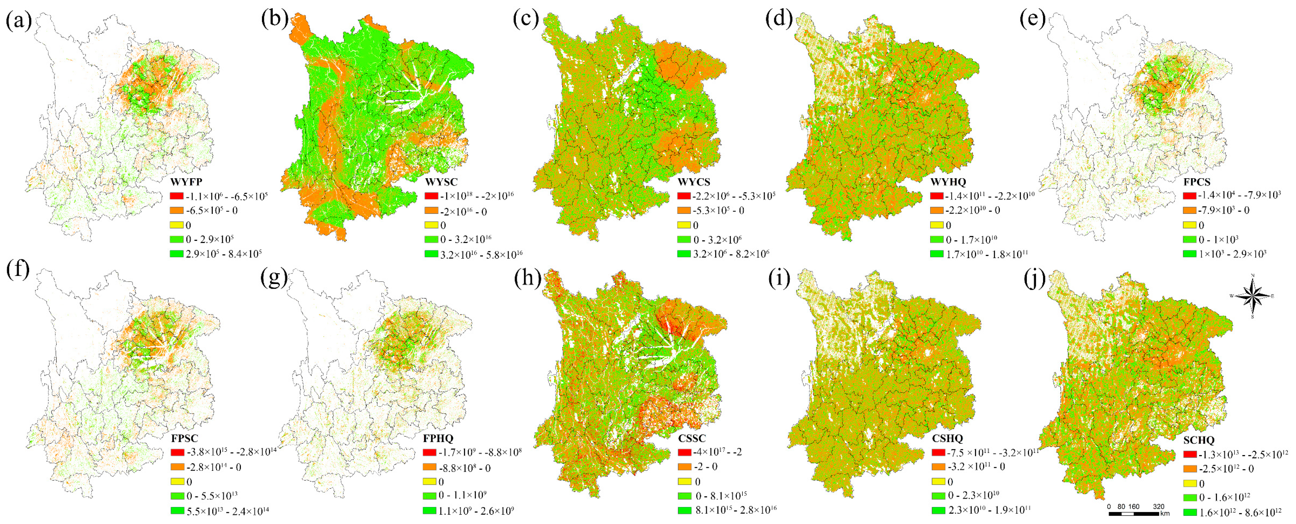
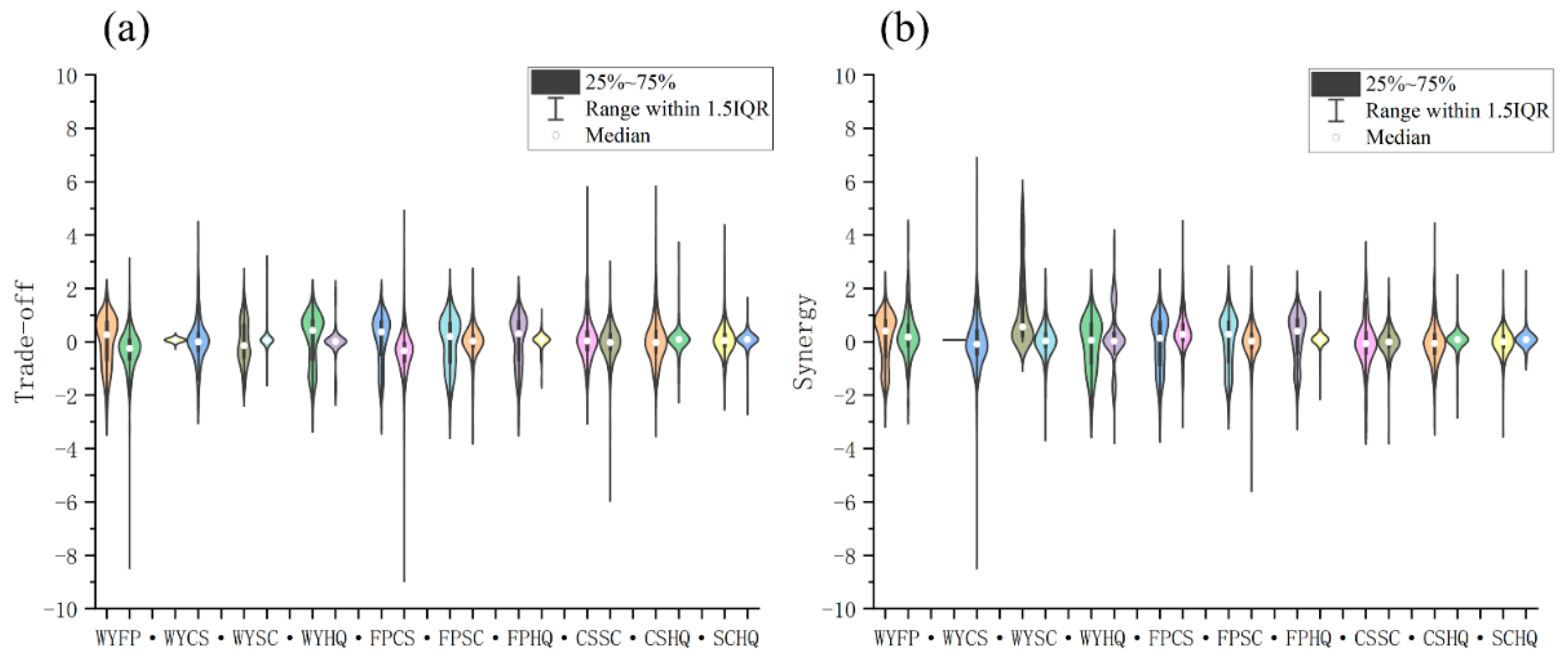
3.2.2. ESTD Results
3.3. Response Curves of ES Trade-Offs/Synergies
4. Discussion
4.1. ES Assessment
4.2. ES Trade-Offs/Synergies
4.3. GAM Response Curves
5. Conclusions
Author Contributions
Funding
Data Availability Statement
Conflicts of Interest
References
- Douglas, I. Ecosystems and Human Well-Being. In Reference Module in Earth Systems and Environmental Sciences; Elsevier: Amsterdam, The Netherlands, 2015; p. B978012409548909206X. ISBN 978-0-12-409548-9. [Google Scholar]
- Fisher, B.; Turner, R.K.; Morling, P. Defining and Classifying Ecosystem Services for Decision Making. Ecol. Econ. 2009, 68, 643–653. [Google Scholar] [CrossRef] [Green Version]
- Chen, H.; Fleskens, L.; Schild, J.; Moolenaar, S.; Wang, F.; Ritsema, C. Using Ecosystem Service Bundles to Evaluate Spatial and Tmporal Impacts of Large-Scale Landscape Restoration on Ecosystem Services on the Chinese Loess Plateau. 2021. Available online: https://www.researchsquare.com/article/rs-273669/v1.pdf (accessed on 23 April 2022).
- Gao, J. Editorial for the Special Issue “Ecosystem Services with Remote Sensing”. Remote Sens. 2020, 12, 2191. [Google Scholar] [CrossRef]
- Felipe-Lucia, M.R.; Comín, F.A.; Bennett, E.M. Interactions Among Ecosystem Services Across Land Uses in a Floodplain Agroecosystem. Ecol. Soc. 2014, 19, art20. [Google Scholar] [CrossRef] [Green Version]
- Bennett, E.M.; Peterson, G.D.; Gordon, L.J. Understanding Relationships among Multiple Ecosystem Services: Relationships among Multiple Ecosystem Services. Ecol. Lett. 2009, 12, 1394–1404. [Google Scholar] [CrossRef]
- Qian, D.; Du, Y.; Li, Q.; Guo, X.; Cao, G. Alpine Grassland Management Based on Ecosystem Service Relationships on the Southern Slopes of the Qilian Mountains, China. J. Environ. Manag. 2021, 288, 112447. [Google Scholar] [CrossRef] [PubMed]
- Shen, J.; Li, S.; Liang, Z.; Liu, L.; Li, D.; Wu, S. Exploring the Heterogeneity and Nonlinearity of Trade-Offs and Synergies among Ecosystem Services Bundles in the Beijing-Tianjin-Hebei Urban Agglomeration. Ecosyst. Serv. 2020, 43, 101103. [Google Scholar] [CrossRef]
- Cord, A.F.; Bartkowski, B.; Beckmann, M.; Dittrich, A.; Hermans-Neumann, K.; Kaim, A.; Lienhoop, N.; Locher-Krause, K.; Priess, J.; Schröter-Schlaack, C.; et al. Towards Systematic Analyses of Ecosystem Service Trade-Offs and Synergies: Main Concepts, Methods and the Road Ahead. Ecosyst. Serv. 2017, 28, 264–272. [Google Scholar] [CrossRef]
- Chen, H.; Fleskens, L.; Schild, J.; Moolenaar, S.; Wang, F.; Ritsema, C. Impacts of Large-Scale Landscape Restoration on Spatio-Temporal Dynamics of Ecosystem Services in the Chinese Loess Plateau. Landsc. Ecol. 2022, 37, 329–346. [Google Scholar] [CrossRef]
- Chiang, A.Y. Generalized Additive Models: An Introduction with R. Technometrics 2007, 49, 360–361. [Google Scholar] [CrossRef]
- Wang, F.; Yuan, X.; Zhou, L.; Liu, S.; Zhang, M.; Zhang, D. Detecting the Complex Relationships and Driving Mechanisms of Key Ecosystem Services in the Central Urban Area Chongqing Municipality, China. Remote Sens. 2021, 13, 4248. [Google Scholar] [CrossRef]
- Pu, H.; Wang, S.; Wang, Z.; Ran, Z.; Jiang, M. Non-Linear Relations between Life Expectancy, Socio-Economic, and Air Pollution Factors: A Global Assessment with Spatial Disparities. Environ. Sci. Pollut. Res. 2022. [Google Scholar] [CrossRef]
- Wahiduzzaman, M.; Luo, J.-J. Modeling of Tropical Cyclone Activity over the North Indian Ocean Using Generalised Additive Model and Machine Learning Techniques: Role of Boreal Summer Intraseasonal Oscillation. Nat. Hazards 2022, 111, 1801–1811. [Google Scholar] [CrossRef]
- Mu, B.; Zhao, X.; Wu, D.; Wang, X.; Zhao, J.; Wang, H.; Zhou, Q.; Du, X.; Liu, N. Vegetation Cover Change and Its Attribution in China from 2001 to 2018. Remote Sens. 2021, 13, 496. [Google Scholar] [CrossRef]
- Tong, X.; Brandt, M.; Yue, Y.; Horion, S.; Wang, K.; Keersmaecker, W.D.; Tian, F.; Schurgers, G.; Xiao, X.; Luo, Y.; et al. Increased Vegetation Growth and Carbon Stock in China Karst via Ecological Engineering. Nat. Sustain. 2018, 1, 44–50. [Google Scholar] [CrossRef]
- Editorial Department of Journal of Remote Sensing. Briefing on “Remote Sensing Scale Effects and Scale Conversion” Forum. J. Remote Sens. 2014, 18, 735–740. [Google Scholar]
- Ran, C.; Wang, S.; Bai, X.; Tan, Q.; Zhao, C.; Luo, X.; Chen, H.; Xi, H. Trade-Offs and Synergies of Ecosystem Services in Southwestern China. Environ. Eng. Sci. 2020, 37, 669–678. [Google Scholar] [CrossRef]
- Chen, Y.; Feng, X.; Fu, B.; Wu, X.; Gao, Z. Improved Global Maps of the Optimum Growth Temperature, Maximum Light Use Efficiency, and Gross Primary Production for Vegetation. J. Geophys. Res. Biogeosci. 2021, 126, e2020JG005651. [Google Scholar] [CrossRef]
- Chen, Y.; Feng, X.; Tian, H.; Wu, X.; Gao, Z.; Feng, Y.; Piao, S.; Lv, N.; Pan, N.; Fu, B. Accelerated Increase in Vegetation Carbon Sequestration in China after 2010: A Turning Point Resulting from Climate and Human Interaction. Glob. Chang. Biol. 2021, 27, 5848–5864. [Google Scholar] [CrossRef]
- Tesfaye, A.; Brouwer, R. Testing Participation Constraints in Contract Design for Sustainable Soil Conservation in Ethiopia. Ecol. Econ. 2012, 73, 168–178. [Google Scholar] [CrossRef]
- Wang, B.; Cheng, W. Effects of Land Use/Cover on Regional Habitat Quality under Different Geomorphic Types Based on InVEST Model. Remote Sens. 2022, 14, 1279. [Google Scholar] [CrossRef]
- Smith, P. Delivering Food Security without Increasing Pressure on Land. Glob. Food Secur. 2013, 2, 18–23. [Google Scholar] [CrossRef]
- Zhang, T.; Zhang, S.; Cao, Q.; Wang, H.; Li, Y. The Spatiotemporal Dynamics of Ecosystem Services Bundles and the Social-Economic-Ecological Drivers in the Yellow River Delta Region. Ecol. Indic. 2022, 135, 108573. [Google Scholar] [CrossRef]
- Li, M.; Zheng, P.; Pan, W. Spatial-Temporal Variation and Tradeoffs/Synergies Analysis on Multiple Ecosystem Services: A Case Study in Fujian. Sustainability 2022, 14, 3086. [Google Scholar] [CrossRef]
- Costanza, R.; de Groot, R.; Braat, L.; Kubiszewski, I.; Fioramonti, L.; Sutton, P.; Farber, S.; Grasso, M. Twenty Years of Ecosystem Services: How Far Have We Come and How Far Do We Still Need to Go? Ecosyst. Serv. 2017, 28, 1–16. [Google Scholar] [CrossRef]
- Pedersen, E.J.; Miller, D.L.; Simpson, G.L.; Ross, N. Hierarchical Generalized Additive Models in Ecology: An Introduction with Mgcv. PeerJ 2019, 7, e6876. [Google Scholar] [CrossRef] [PubMed] [Green Version]
- Rau, A.-L.; von Wehrden, H.; Abson, D.J. Temporal Dynamics of Ecosystem Services. Ecol. Econ. 2018, 151, 122–130. [Google Scholar] [CrossRef]
- Li, W.; Wang, W.; Chen, J.; Zhang, Z. Assessing Effects of the Returning Farmland to Forest Program on Vegetation Cover Changes at Multiple Spatial Scales: The Case of Northwest Yunnan, China. J. Environ. Manag. 2022, 304, 114303. [Google Scholar] [CrossRef] [PubMed]
- Li, F.; Zhou, W.; Shao, Z.; Zhou, X. Effects of Ecological Projects on Vegetation in the Three Gorges Area of Chongqing, China. J. Mt. Sci. 2022, 19, 121–135. [Google Scholar] [CrossRef]
- Liu, S.; Liao, Q.; Xiao, M.; Zhao, D.; Huang, C. Spatial and Temporal Variations of Habitat Quality and Its Response of Landscape Dynamic in the Three Gorges Reservoir Area, China. Int. J. Environ. Res. Public Health 2022, 19, 3594. [Google Scholar] [CrossRef]
- Li, C.; Qi, J.; Feng, Z.; Yin, R.; Guo, B.; Zhang, F.; Zou, S. Quantifying the Effect of Ecological Restoration on Soil Erosion in China’s Loess Plateau Region: An Application of the MMF Approach. Environ. Manag. 2010, 45, 476–487. [Google Scholar] [CrossRef]
- Vári, Á.; Kozma, Z.; Pataki, B.; Jolánkai, Z.; Kardos, M.; Decsi, B.; Pinke, Z.; Jolánkai, G.; Pásztor, L.; Condé, S.; et al. Disentangling the Ecosystem Service ‘Flood Regulation’: Mechanisms and Relevant Ecosystem Condition Characteristics. Ambio 2022, 1–16. [Google Scholar] [CrossRef]
- Battisti, L.; Corsini, F.; Gusmerotti, N.M.; Larcher, F. Management and Perception of Metropolitan Natura 2000 Sites: A Case Study of La Mandria Park (Turin, Italy). Sustainability 2019, 11, 6169. [Google Scholar] [CrossRef] [Green Version]
- Battisti, L.; Pomatto, E.; Larcher, F. Assessment and Mapping Green Areas Ecosystem Services and Socio-Demographic Characteristics in Turin Neighborhoods (Italy). Forests 2019, 11, 25. [Google Scholar] [CrossRef] [Green Version]
- Berglihn, E.C.; Gómez-Baggethun, E. Ecosystem Services from Urban Forests: The Case of Oslomarka, Norway. Ecosyst. Serv. 2021, 51, 101358. [Google Scholar] [CrossRef]
- Jopke, C.; Kreyling, J.; Maes, J.; Koellner, T. Interactions among Ecosystem Services across Europe: Bagplots and Cumulative Correlation Coefficients Reveal Synergies, Trade-Offs, and Regional Patterns. Ecol. Indic. 2015, 49, 46–52. [Google Scholar] [CrossRef]
- Pan, J.; Wei, S.; Li, Z. Spatiotemporal Pattern of Trade-Offs and Synergistic Relationships among Multiple Ecosystem Services in an Arid Inland River Basin in NW China. Ecol. Indic. 2020, 114, 106345. [Google Scholar] [CrossRef]
- Vallet, A.; Locatelli, B.; Levrel, H.; Brenes Pérez, C.; Imbach, P.; Estrada Carmona, N.; Manlay, R.; Oszwald, J. Dynamics of Ecosystem Services during Forest Transitions in Reventazón, Costa Rica. PLoS ONE 2016, 11, e0158615. [Google Scholar] [CrossRef] [Green Version]
- Feng, Q.; Zhao, W.; Fu, B.; Ding, J.; Wang, S. Ecosystem Service Trade-Offs and Their Influencing Factors: A Case Study in the Loess Plateau of China. Sci. Total Environ. 2017, 607–608, 1250–1263. [Google Scholar] [CrossRef]
- Obiang Ndong, G.; Villerd, J.; Cousin, I.; Therond, O. Using a Multivariate Regression Tree to Analyze Trade-Offs between Ecosystem Services: Application to the Main Cropping Area in France. Sci. Total Environ. 2021, 764, 142815. [Google Scholar] [CrossRef]
- Zhao, J.; Li, C. Investigating Ecosystem Service Trade-Offs/Synergies and Their Influencing Factors in the Yangtze River Delta Region, China. Land 2022, 11, 106. [Google Scholar] [CrossRef]
- Xu, S.; Liu, Y.; Wang, X.; Zhang, G. Scale Effect on Spatial Patterns of Ecosystem Services and Associations among Them in Semi-Arid Area: A Case Study in Ningxia Hui Autonomous Region, China. Sci. Total Environ. 2017, 598, 297–306. [Google Scholar] [CrossRef] [PubMed]
- Gong, J.; Liu, D.; Zhang, J.; Xie, Y.; Cao, E.; Li, H. Tradeoffs/Synergies of Multiple Ecosystem Services Based on Land Use Simulation in a Mountain-Basin Area, Western China. Ecol. Indic. 2019, 99, 283–293. [Google Scholar] [CrossRef]
- Yang, Y.; Li, M.; Feng, X.; Yan, H.; Su, M.; Wu, M. Spatiotemporal Variation of Essential Ecosystem Services and Their Trade-off/Synergy along with Rapid Urbanization in the Lower Pearl River Basin, China. Ecol. Indic. 2021, 133, 108439. [Google Scholar] [CrossRef]
- Peng, L.; Wang, X. What Is the Relationship between Ecosystem Services and Urbanization? A Case Study of the Mountainous Areas in Southwest China. J. Mt. Sci. 2019, 16, 2867–2881. [Google Scholar] [CrossRef]
- Luo, R.; Yang, S.; Wang, Z.; Zhang, T.; Gao, P. Impact and Trade off Analysis of Land Use Change on Spatial Pattern of Ecosystem Services in Chishui River Basin. Environ. Sci. Pollut. Res. 2022, 29, 20234–20248. [Google Scholar] [CrossRef]
- Chen, T.; Peng, L.; Wang, Q. Response and Multiscenario Simulation of Trade-Offs/Synergies among Ecosystem Services to the Grain to Green Program: A Case Study of the Chengdu-Chongqing Urban Agglomeration, China. Environ. Sci. Pollut. Res. 2022, 29, 33572–33586. [Google Scholar] [CrossRef]
- Qiu, M.; Van de Voorde, T.; Li, T.; Yuan, C.; Yin, G. Spatiotemporal Variation of Agroecosystem Service Trade-Offs and Its Driving Factors across Different Climate Zones. Ecol. Indic. 2021, 130, 108154. [Google Scholar] [CrossRef]
- Watson, S.C.L.; Newton, A.C.; Ridding, L.E.; Evans, P.M.; Brand, S.; McCracken, M.; Gosal, A.S.; Bullock, J.M. Does Agricultural Intensification Cause Tipping Points in Ecosystem Services? Landsc. Ecol. 2021, 36, 3473–3491. [Google Scholar] [CrossRef]
- Xue, L.; Liang, H. Polynomial Spline Estimation for a Generalized Additive Coefficient Model. Scand. J. Stat. 2010, 37, 26–46. [Google Scholar] [CrossRef] [Green Version]
- Wood, S.N. Fast Stable Direct Fitting and Smoothness Selection for Generalized Additive Models. J. R. Stat. Soc. B 2008, 70, 495–518. [Google Scholar] [CrossRef] [Green Version]
- Wood, S.N.; Goude, Y.; Shaw, S. Generalized Additive Models for Large Data Sets. J. R. Stat. Soc. C 2015, 64, 139–155. [Google Scholar] [CrossRef] [Green Version]


| ES | Calculation or Formula Model | Parameters and Processing |
|---|---|---|
| Water Yield | Y(x) = P(x) − AET(x) | Y(x) is the average annual water yield, P(x) is the average annual precipitation, and AET is actual evapotranspiration. |
| Carbon Sequestration | PAR is calculated by multiplying CERES solar radiation and the monthly PAR/SW ratio derived from the BESS data set. and (i.e., maximum LUE and optimum growth temperature) refer to various flux measurements and sun-induced chlorophyll fluorescence values [19,20]. | |
| Soil Conservation | The Sediment Delivery Ratio model | RKLS is the potential soil erosion (t) in the study area under specific landscape and climate conditions, USLE is the actual amount of soil erosion (t) after taking into account the interception effect of vegetation and the implementation of management engineering measures, SD is soil retention (t), R is rainfall erosion force, K is soil erodibility, LS is the slope length slope factor, C is the vegetation cover factor, and P is the soil conservation measure factor. |
| Habitat Quality | The Habitat Quality model | Qxj is the habitat quality index of x grids in j habitats, Hj is the habitat suitability score of j habitats between 0 and 1, k is the half-saturation constant which is usually taken as 1/2 of the habitat degradation index, and z is the normalization constant, which is usually taken as the default value of 2.5. |
| Food Production | Gi is the food production service of raster I, Gsum is the total food production of each county, NDVIsum is the sum of NDVI of arable land-like elements in the county, and NDVIi is the NDVI of raster i. |
| WY-FP | WY-CS | WY-SC | WY-HQ | FP-CS | FP-SC | FP-HQ | CS-SC | CS-HQ | SC-HQ | |
|---|---|---|---|---|---|---|---|---|---|---|
| Trade-off | 50.02% | 45.23% | 30.65% | 51.05% | 49.23% | 52.08% | 50.89% | 46.72% | 51.46% | 51.86% |
| Synergy | 49.98% | 54.77% | 69.35% | 48.95% | 50.77% | 47.92% | 49.11% | 53.28% | 48.54% | 48.14% |
| WY-FP | WY-CS | WY-SC | WY-HQ | FP-CS | FP-SC | FP-HQ | CS-SC | CS-HQ | SC-HQ | |||||||||||
|---|---|---|---|---|---|---|---|---|---|---|---|---|---|---|---|---|---|---|---|---|
| ES-change | WY | FP | WY | CS | WY | SC | WY | HQ | FP | CS | FP | SC | FP | HQ | CS | SC | CS | HQ | SC | HQ |
| edf | 6.42 | 1.42 | 4.71 | 1.00 | 6.08 | 1.00 | 7.57 | 1.00 | 1.00 | 1.00 | 6.17 | 1.00 | 1.00 | 7.10 | 8.98 | 1.00 | 6.44 | 1.00 | 7.88 | 1.00 |
| Kindex | 0.99 | 1.01 | 0.94 | 0.90 | 1.01 | 1.02 | 1.02 | 1.00 | 1.00 | 1.02 | 1.03 | 1.00 | 1.00 | 1.05 | 1.00 | 1.00 | 0.99 | 1.01 | 1.01 | 1.00 |
Publisher’s Note: MDPI stays neutral with regard to jurisdictional claims in published maps and institutional affiliations. |
© 2022 by the authors. Licensee MDPI, Basel, Switzerland. This article is an open access article distributed under the terms and conditions of the Creative Commons Attribution (CC BY) license (https://creativecommons.org/licenses/by/4.0/).
Share and Cite
Huang, Q.; Peng, L.; Huang, K.; Deng, W.; Liu, Y. Generalized Additive Model Reveals Nonlinear Trade-Offs/Synergies between Relationships of Ecosystem Services for Mountainous Areas of Southwest China. Remote Sens. 2022, 14, 2733. https://doi.org/10.3390/rs14122733
Huang Q, Peng L, Huang K, Deng W, Liu Y. Generalized Additive Model Reveals Nonlinear Trade-Offs/Synergies between Relationships of Ecosystem Services for Mountainous Areas of Southwest China. Remote Sensing. 2022; 14(12):2733. https://doi.org/10.3390/rs14122733
Chicago/Turabian StyleHuang, Qi, Li Peng, Kexin Huang, Wei Deng, and Ying Liu. 2022. "Generalized Additive Model Reveals Nonlinear Trade-Offs/Synergies between Relationships of Ecosystem Services for Mountainous Areas of Southwest China" Remote Sensing 14, no. 12: 2733. https://doi.org/10.3390/rs14122733
APA StyleHuang, Q., Peng, L., Huang, K., Deng, W., & Liu, Y. (2022). Generalized Additive Model Reveals Nonlinear Trade-Offs/Synergies between Relationships of Ecosystem Services for Mountainous Areas of Southwest China. Remote Sensing, 14(12), 2733. https://doi.org/10.3390/rs14122733