Article

The Applicability of LandTrendr to Surface Water Dynamics: A Case Study of Minnesota from 1984 to 2019 Using Google Earth Engine

by
Audrey C. Lothspeich
and
Joseph F. Knight
*
Department of Forest Resources, University of Minnesota, 1530 Cleveland Ave. N, St. Paul, MN 55108, USA
*
Author to whom correspondence should be addressed.
Remote Sens. 2022, 14(11), 2662; https://doi.org/10.3390/rs14112662
Submission received: 21 April 2022 / Revised: 20 May 2022 / Accepted: 30 May 2022 / Published: 2 June 2022
(This article belongs to the Special Issue Advances in Geospatial Data Analysis for Change Detection)

Abstract

:
The means to accurately monitor wetland change over time are crucial to wetland management. This paper explores the applicability of LandTrendr, a temporal segmentation algorithm designed to identify significant interannual trends, to monitor wetlands by modeling surface water presence in Minnesota from 1984 to 2019. A time series of harmonized Landsat and Sentinel-2 data in the spring is developed in Google Earth Engine, and calculated to sub-pixel water fraction. The optimal parameters for modeling this time series with LandTrendr are identified by minimizing omission of known surface water locations, and the result of this optimal model of sub-pixel water fraction is evaluated against reference images and qualitatively. Accuracy of this method is high: overall accuracy is 98% and producer’s and user’s accuracies for inundation are 82% and 88% respectively. Maps summarizing the trendlines of multiple pixels, such as frequency of inundation over the past 35 years, also show LandTrendr as applied here can accurately model long-term trends in surface water presence across wetland types. However, the tendency of omission for more variable prairie pothole wetlands and the under-prediction of inundation for small or emergent wetlands suggests the algorithm will require careful development of the segmented time series to capture inundated conditions more accurately.

Graphical Abstract

1. Introduction

To ensure effective management, it is increasingly important to understand wetlands within their temporal context. In the past 200 years, more than 50% of original wetland area in the United States has been drained for development or agriculture. However, this conversion is not uniform across the country, creating markedly different distributions of wetlands over time and space. Estimates of wetlands loss in the United States since the 1780s range from 20 to 70% of their original extent [1], with peatlands remaining relatively intact, and the prairie pothole region with as little as five percent of their original land area [1,2,3]. These losses affect not only the locations where conversion occurred, but the functions of remaining wetlands. Landscape-level studies of wetland connectivity indicate that changes to wetland distribution affect the quality of habitat provided by wetlands [4], as well as their ability to remove nitrate [5,6]. For example, Cheng et al. found that an increase in wetland area of only 10% with adequate connectivity could decrease nitrogen loading in affected wetlands by as much as 54% [5]. While wetlands are now more protected from direct conversion due to the Clean Water Act and no-net-loss policies, these protections themselves can contribute to shifts in wetland spatial distribution [7], vegetation [8], and temporal presence [9]. For instance, while the overall wetland area may remain stable under no-net-loss policies, a noted trend is toward a loss in quality of function, as the wetlands most easily converted for development and the wetlands most easily created during mitigation efforts tend to support different amounts of vegetation and provide different functions [7,10]. Additionally, climate change is affecting wetlands, as changing precipitation patterns alter the timing and duration of saturating conditions for many wetlands [11,12]. As such, wetlands have changed and will continue to change as a result of multiple processes, with direct consequences to their functions.
Taking advantage of the long time series of imagery at a medium resolution and frequent revisit time, many have used the Landsat imagery archive to characterize wetland change over time [13,14,15,16,17,18]. Commonly, previous efforts have sought to identify changes in surface water extent, creating maps of surface water presence/absence with spectral indices [13,14,15,16,19], such as the Dynamic Surface Water Extent (DSWE) [20]. Such applications have been shown to be accurate across wetland types and readily scalable over large areas (such the entire continent of Australia [14]). Further, models based on surface water extent have been shown to be a useful proxy for larger trends in wetland disturbance, such as rates of development [16]. However, such methods are limited to directly monitoring only wetlands that contain large amounts of visible surface water, with poor performance in emergent or very small wetlands. Additionally, they capture only the most extreme changes to wetlands, missing more subtle changes in wetness than simply water presence or absence. Other efforts have focused on classifying wetlands through time [21,22]. For example, Mahdianpari et al. [21] used a random forest model to predict the temporal distribution of bogs, fens, and marshes, producing both approximate wetland inventories for Canada and rates of transition between wetland types. Classification-based methods capture more types of wetlands and change than those based on surface water by explicitly modeling wetlands with emergent vegetation. However, these methods have also exhibited low accuracies for wetland classes. The same research by Mahdianpari [21] noted accuracies as low as 50% for different wetland classes, making the signal-to-noise ratio relatively low for confident assessment of spatiotemporal wetlands trends. Some of the most detailed and accurate temporal models use spectral mixture analysis (SMA), in which samples of “pure” spectral endmembers (e.g., water, wetland vegetation) are used to identify the composition of mixed pixels [17,23,24,25]. Unlike surface water extent or classification-based methods, SMA produces continuous estimates of the relative amounts of different components of a pixel over time. Due to the increase in spectral detail with continuous data, SMA results have been very accurate, capable of even accurately modeling the hydropattern of wetlands [17]. However, SMA models have been limited to only small regions, as maintaining consistency among spectral endmembers becomes challenging at larger scales [17,25]. Given the tradeoffs of these approaches, there is a need for a detailed yet broadly applicable means of assessing wetland change over time.
A potential method for improving our understanding wetland dynamics is the LandTrendr algorithm, as implemented in Google Earth Engine [26,27]. LandTrendr is a temporal segmentation algorithm. Given a time series of satellite imagery and a set of parameters controlling model fit, it statistically identifies which years in the time series are inflection points and linearly regresses the trend-line between them (Figure 1). LandTrendr was originally developed for forestry applications. It is most commonly applied to track recovery of vegetation: forests and, to a lesser extent, wetland vegetation have been monitored using spectral indices with LandTrendr [26,28,29,30,31]. While it was very recently applied to surface water dynamics by Chai et al. [32], this study used LandTrendr for a subset of the Landsat catalog and over a more homogenous ecoregion. As such, LandTrendr’s value in describing temporal dynamics of wetlands generally, over larger time ranges and more diverse wetlands, can be better established. An important advantage of LandTrendr is its ability to create continuous trendlines of an index for each pixel (similar to SMA) that normalize spurious inter-annual variation [27]. These fitted trendline values are especially valuable because they can improve the accuracy of long time series wetland dynamics compared to other methods of temporal modeling. By regressing values between identified inflection years, LandTrendr can normalize inter-annual noise in trendlines due to inconsistent image samples between years or small climate variations, and fill gaps in the time series [26,27]. At regional scales, key inflection years and the trends between them can be easily summarized across many pixels, reducing temporal patterns of individual pixels into larger, landscape-level patterns of wetland surface water. As such, LandTrendr has the potential to improve wetland management from the local to regional scales, giving both specific information for locations and trends over time.
Given these potential benefits to time series analysis with LandTrendr, this research seeks to explore the applicability of LandTrendr to understanding wetland surface water dynamics. Specifically, this research develops a LandTrendr model of sub-pixel water fraction dynamics in Minnesota from 1984 to 2019 with Google Earth Engine, and evaluates its accuracy for wetland management applications at different scales.

2. Materials and Methods
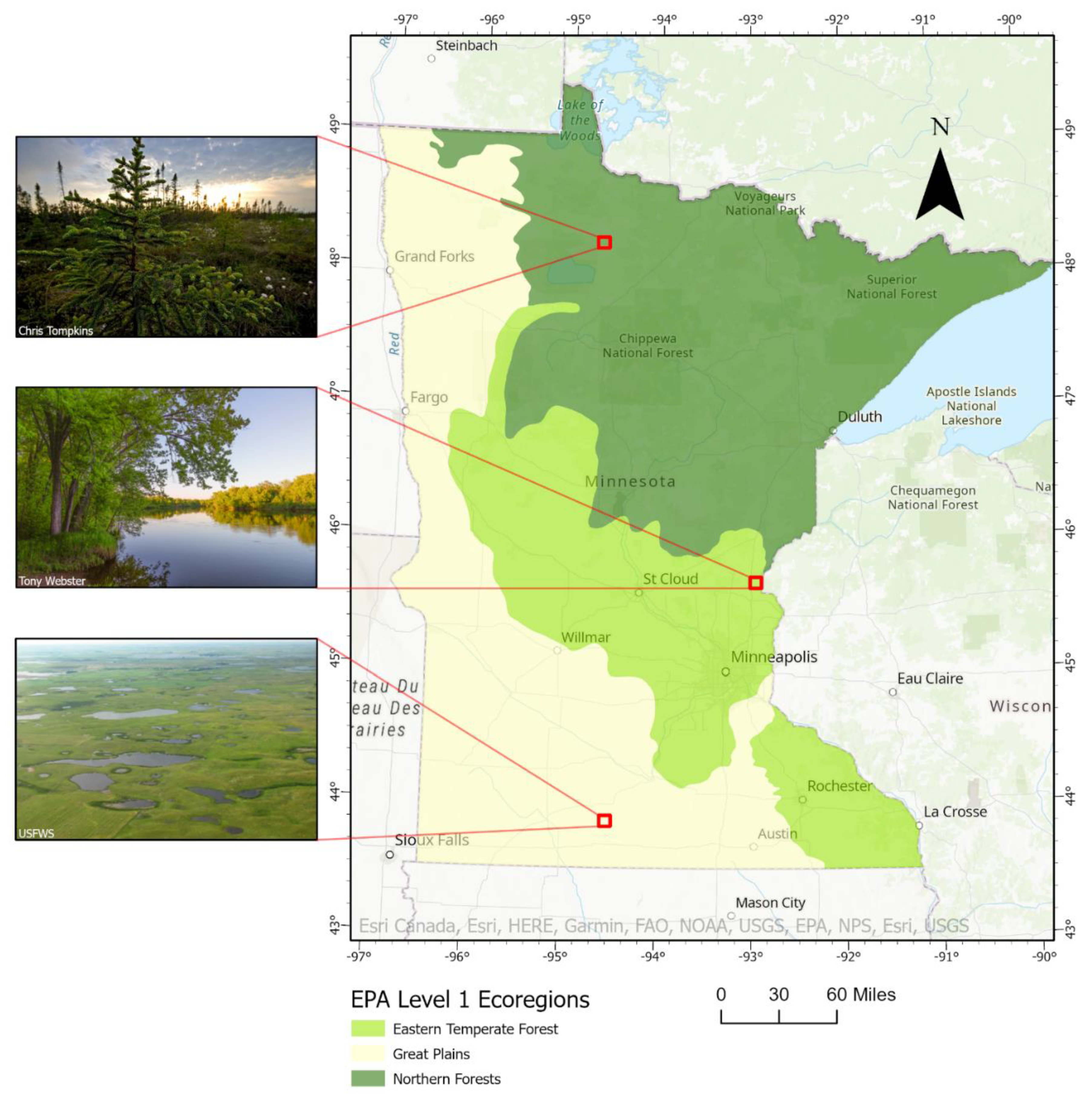
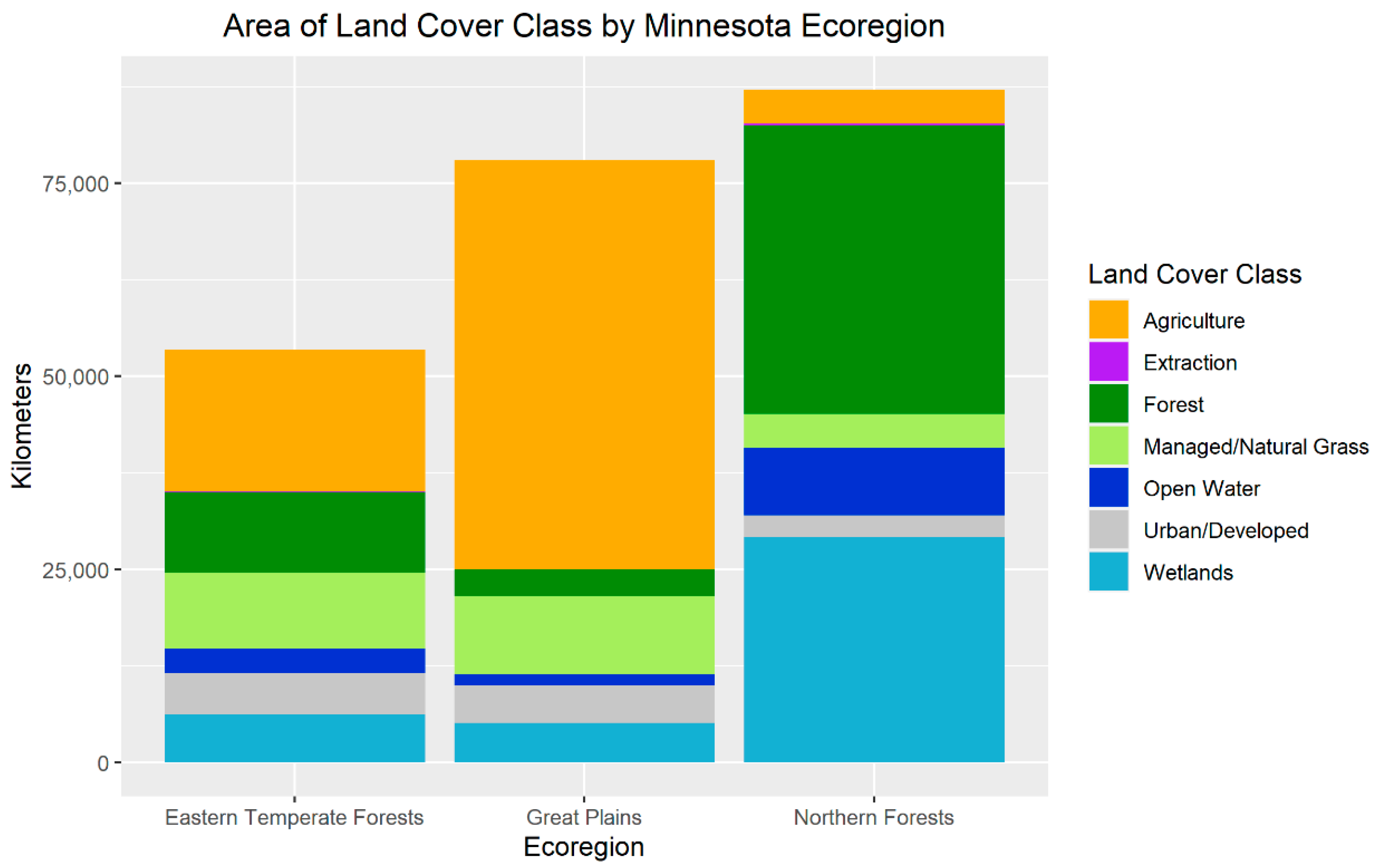
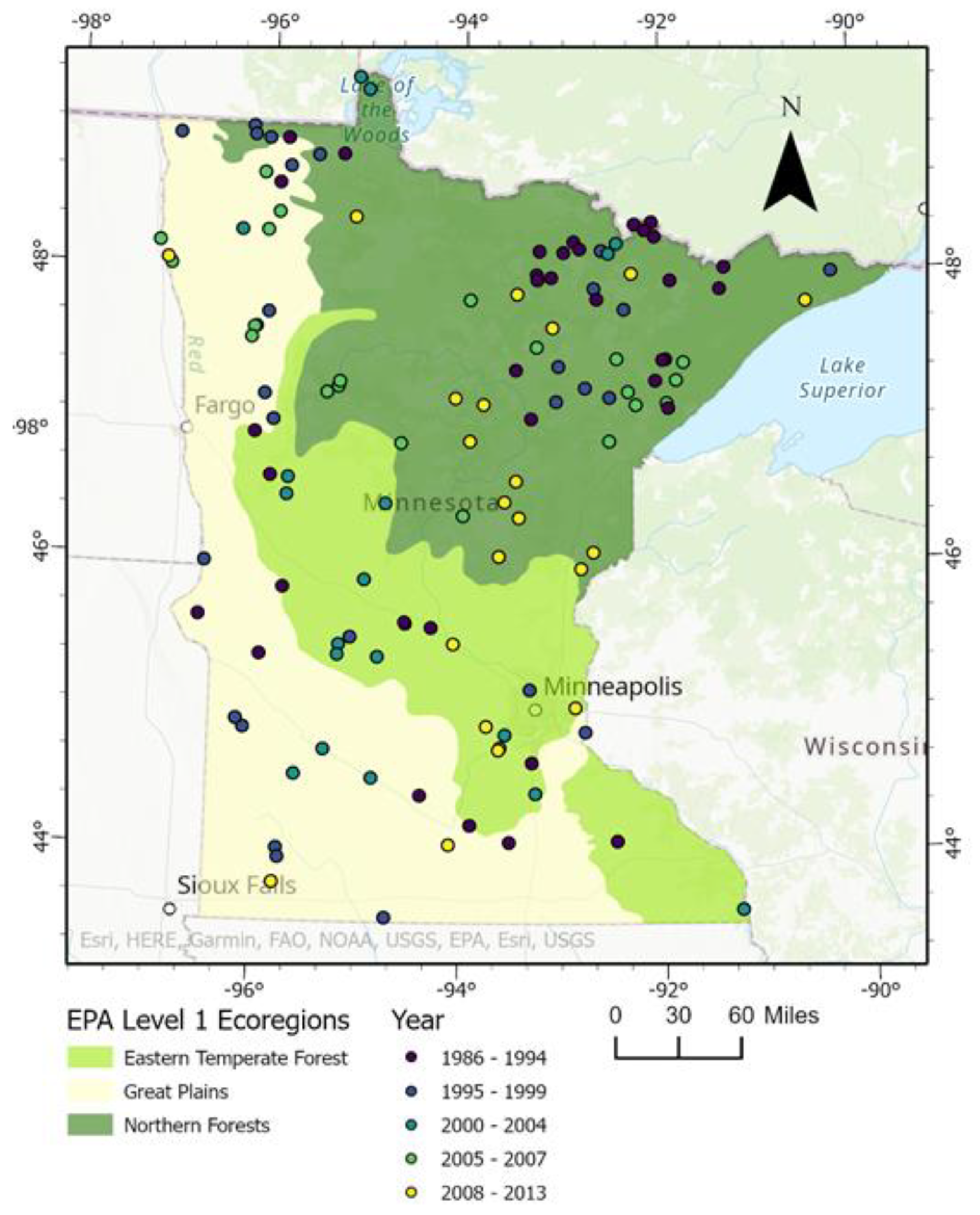
2.1. Study Area

Minnesota contains more than 10.6 million acres of wetlands (13 million acres including deep-water habitat) [34] which span a broad range of types and ecosystem contexts. The most common types of wetlands in the state are forested, followed by emergent and scrub-shrub dominated wetlands. The majority of these wetlands are saturated or temporarily inundated as opposed to persistently inundated with visible surface water [34]. However, there are distinct geographic differences in wetland type and the challenges to observing them remotely (Figure 2 and Figure 3). The northern and northeastern portions of the state are dominated by forested wetlands and extensive areas of peatland, the majority of which has remained since pre-settlement as the region has limited development and agriculture (Figure 3) [34]. These wetlands are largely palustrine and characterized by dark, persistent vegetation (e.g., coniferous forests) and saturated soils. In such wetlands, visible inundation occurs only rarely, if at all [34]. As these wetlands tend to lack visible surface water and are obscured by vegetation for much of the year, pixel mixing or obscuration limits the ability to identify water at these locations. Southern and western portions of the state are characterized by many depressional wetlands due to recent glaciation. These depressions, known as prairie potholes, can range in size and degree of inundation, including small wet prairies to large marshes ringed by emergent vegetation. The degree of inundation in these depressions is also highly variable [35,36], sensitive to annual climate variations, such as drought, and varying seasonally. This high degree of variability in surface water extent in these wetlands poses a challenge to consistent monitoring, since crucial surface water conditions may be missed due to clouds or gaps between satellite revisits [36]. While the prairie pothole region had many wetlands pre-settlement, this region has been the most affected by development and especially drainage for cultivation. Indeed, some parts of this region have lost more than 90% of their original wetland area to agriculture, and many wetlands that remain this region are in active cultivation, affecting the context in which surface water is observed (Figure 3) [3]. The transitional ecotone between these two regions includes a broad mix of land cover and wetland types (Figure 3), including bogs, lakes, and forested wetlands as in the northern portions of the state, as well as marshes and depressional wetlands similar to the prairie pothole region [34]. As such, Minnesota contains a wide range of wetland types, hydrologic regimes, and landscape contexts to test the performance of automated monitoring methods against.

2.2. Satellite Imagery Acquisition and Pre-Processing

A satellite image time series from 1984 to 2019 was created in Google Earth Engine to characterize surface water change over time. Images were compiled from Tier 1 catalogs of Landsat 4 ETM, Landsat 5 ETM, Landsat 7 ETM+, Landsat 8 OLI, and Sentinel-2 MSI surface reflectance [37,38,39]. For each year, images over the state of Minnesota were selected between the calendar dates of 1 May and 30 June. This time period was selected to represent spring conditions with leaf-off and near maximum water presence due to snowmelt and spring precipitation, as well as minimize within-year variability in captured conditions. Since most years included images from multiple satellite systems, images were harmonized between sensors [40,41]. This included topographic and illumination correction using a bidirectional reflectance distribution function [42] and reprojection to UTM Zone 15 and 30-m resolution so that each image’s pixels were aligned. As different sensors also have different wavelength definitions for each band, Landsat 4, 5, 7, and Sentinel-2 images were linearly transformed such that all bands were made consistent with Landsat 8 OLI [40,43]. Additionally, all images were masked to ensure accurate modeling of surface water. Using the pixel quality mask provided by Google Earth Engine, the images were masked of snow, cloud, cirrus, cloud shadow, and saturated pixels on a pixel-by-pixel basis. Developed areas were also masked using the 2013–2014 land cover and impervious surface dataset for Minnesota [44]. This yielded an average of four images contributing to a pixel’s composite in a given year. However, pixels with a large number of overlapping images had as many as 15 images contributing to the annual composite on average, and some pixels as few as 2 (Supplementary Materials Section S1).

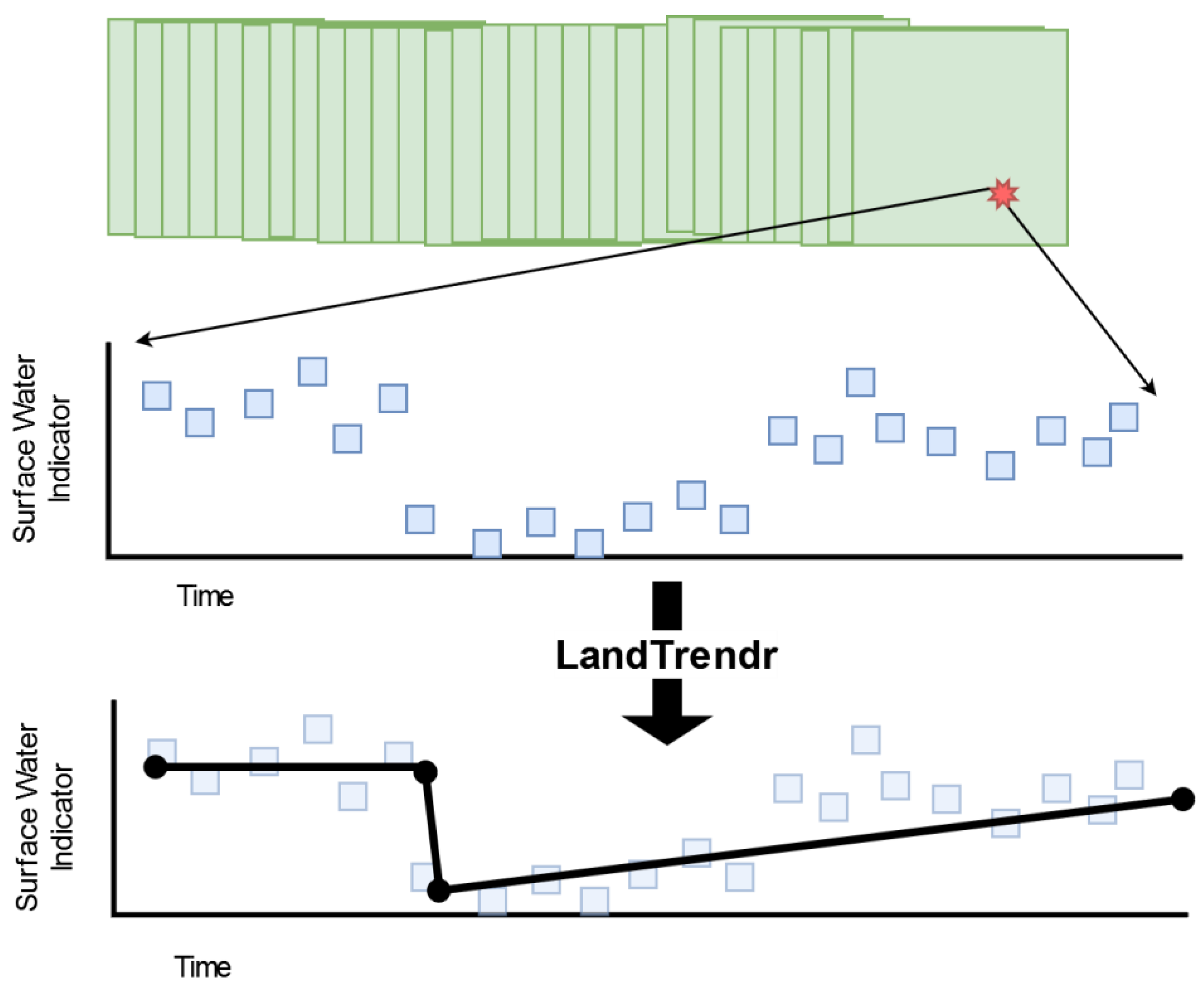
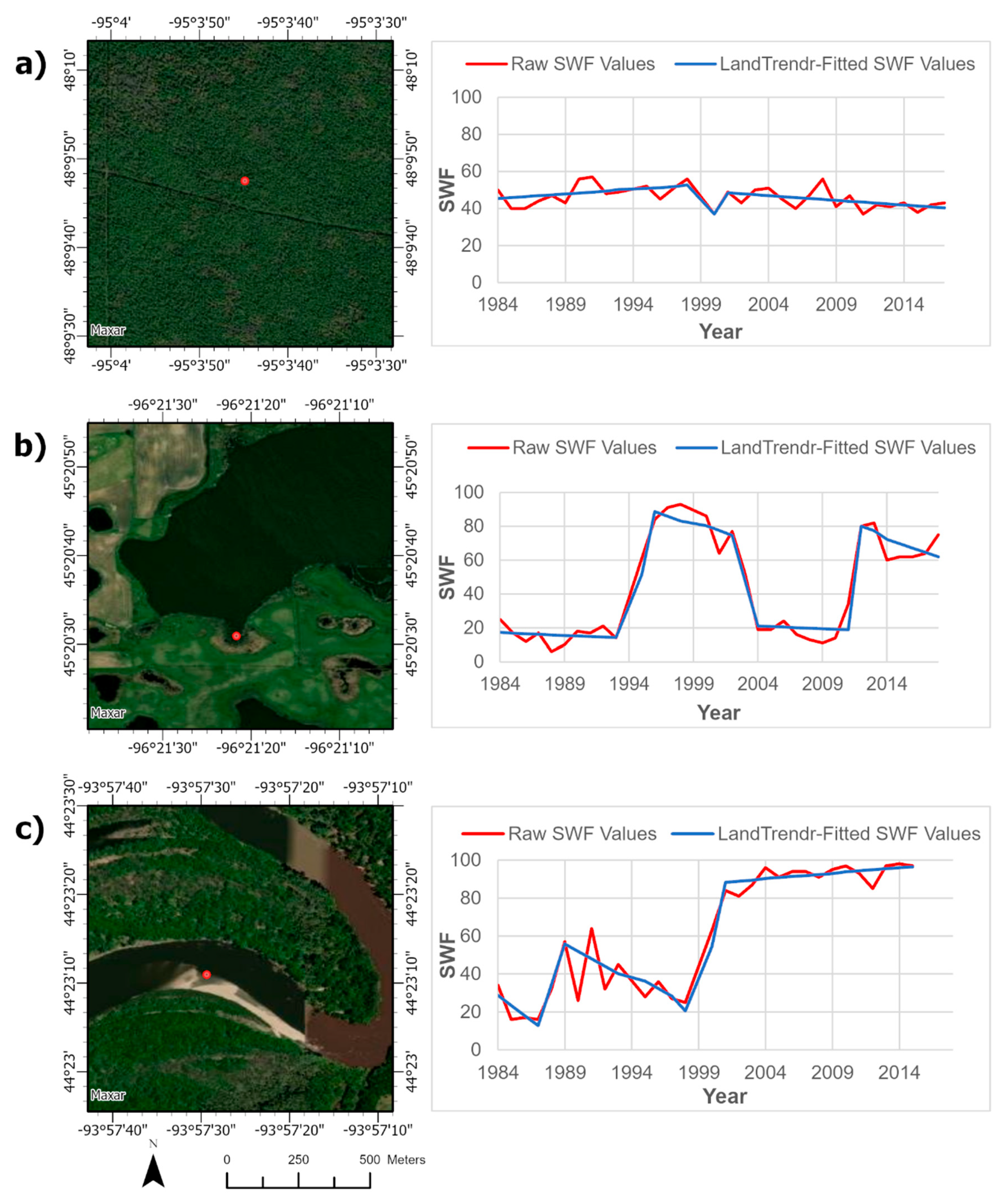
2.3. Creation of the Wetland Time Series

LandTrendr expects a set of annual composites, one image per year, to segment over time [26]. To create annual composites indicative of surface water versus vegetation presence, the harmonized time series was calculated to sub-pixel water fraction (SWF) using a modified version of the algorithm described by De Vries et al. [45]. The SWF algorithm uses a self-trained random forest classifier to predict what percent of a pixel is surface water. Training data are created from a set of raw band values and spectral indices, and the predicted variable is binary surface water presence/absence indicated by the DSWE v2 [46]. Both the training data and predicted variable are coarsened to a lower resolution for training the random forest, so that when the trained model is applied back to the original harmonized time series it yields percent inundation for pixels at the 30 m scale (Figure 4).
Each image in the harmonized time series was calculated to a set of band values and spectral indices to serve as training data (Table 1). This included the raw band values and spectral indices used by De Vries et al. [45] as well as two additional variables intended to create more stable predictions of SWF interannually. The first additional variable was the topographic position index [47] calculated from the HydroSHEDs DEM in Google Earth Engine [48] to increase detection of narrow river features. The second additional variable was the day of year each image was sensed to account for different imagery dates in the sample period at a location in different years. DSWE was calculated for each image in the time series, then reclassified to binary surface water presence or absence. DSWE uses a set of spectral threshold tests to assign four classes: upland, open water, and two partial water classes. Following the recommendations of Jones [46] that conservative estimates perform better in coniferous forests, different definitions of surface water presence from DSWE were applied across Minnesota based on EPA Level 1 ecoregions. In the Northern Forests ecoregion, open water and only the higher-confidence partial water class were considered inundated. In other regions, open water and both partial water classes were considered inundated. As DSWE class was often different between images of the same location at different points in time, the final designation was based on majority: if greater than or equal to 50% of images within the spring period were inundated according to DSWE, that pixel was considered inundated. The final result was a binary mask of water presence for each year.
All training data layers and the DSWE water mask were rescaled to a coarser 150-m resolution for model-training, such that all indices were averaged over a 22,500 square meter neighborhood and water presence value ranged from zero to one. The rescaled training data were then sampled through time and across percent surface water conditions. For each year, a stratified random sample was taken of ~200 points per 10 percent surface water presence. For example, ~200 points had percent surface water values ranging from 0–9%, ~200 pts from 10–19% surface water, etc. The resulting sample of 91,000 points was then used to train a random forest regression model with 500 trees and a 0.05 bag fraction per tree, with all other variables using the default random forest as implemented in Google Earth Engine [49] to predict percent surface water presence. The trained model was then applied to the original, harmonized time series of satellite imagery. Within each year, the medoid predicted SWF for a pixel was chosen to create that year’s annual composite, giving a statewide estimate of SWF at the 30-m scale for each year from 1984 to 2019 which was used as the time series in LandTrendr.
Table 1. Spectral indices used in the SWF algorithm. These indices include those originally suggested by De Vries et al. [45], and those proposed here for use with LandTrendr (identified with an asterisk). These indices were used to train a random forest model in the SWF algorithm to identify percent surface water within a pixel.
Index:Formula:Source:
Tasseled-cap Greenness(−0.2941)B1 + (−0.243)B2 + (−0.5424)B3 + 0.7276B4 + 0.0713B5 + (−0.1608)B6[50]
Tasseled-cap Wetness0.1511B1 + 0.1973B2 + 0.3283B3 + 0.3407B4 + (−0.7117)B5 + (−0.4559)B6[50]
Tasseled-cap Brightness0.3029B1 + 0.2786B2 + 0.4733B3 + 0.5599B4 + 0.508B5 + 0.1872B6[50]
Normalized Difference
Wetness Index
(Green − NIR)/(Green + NIR)[51]
Modified Normalized Difference Wetness Index(Green − SWIR1)/(Green + SWIR1)[52]
Normalized Difference Vegetation Index(NIR − Red)/(NIR + Red)[53]
Topographic Position Index *Dem − FocalMean(dem, radius = 30 pixels)[47]
Day of Year *Julian date within a year

2.4. Parameterization of LandTrendr

The LandTrendr implementation in Google Earth Engine has a variety of parameters to control the allowable temporal relationships of the final model, some of which required optimization to apply to wetland inundation dynamics [27]. The parameter to mask out pixels with time series that are too incomplete for an accurate temporal segmentation (minObservationsNeeded) was held constant at 31. This number of observations is still relatively robust compared to the maximum length of the time series, and a more stringent threshold would exclude large portions of the state from modeling. Additionally, the parameter to prevent one year recovery segments (preventOneYearRecovery) was held constant as false, as there is no expected control on rates of inundation change as may be expected with other systems such as reforestation. For all remaining parameters (maxSegments, spikeThreshold, recoveryThreshold, pvalThreshold, bestModelProportion, and vertexCountOvershoot), a range of parameter values (with the other variables held constant) were tested to find the optimal value to fit wetland inundation dynamics. For example, the parameter controlling the maximum number of segments in the model (maxSegments) was tested with values from 2–13, and a value of 11 was selected to maximize accuracy and minimize model fit time.
Parameter values were chosen to minimize the omission of wetlands with persistent surface water as described in Minnesota’s updated NWI. A location in the NWI was expected to have surface water if it had a water regime class of semi-permanently flooded (F), intermittently exposed (G), or permanently flooded (H). LandTrendr was fitted with each parameter setting within a range, then assessed for inundation in the years 2008 to 2015, which were the same years of imagery on which the updated NWI was based. If a 30 m pixel expected to be inundated according to the NWI did not have at least 50% predicted SWF for the majority of the years between 2008 and 2015, it was considered omission. Using this process, a set of optimal LandTrendr parameters for wetland surface water dynamics over the 1984 to 2019 time period was identified and used as the LandTrendr settings in all subsequent results (Table 2, Supplementary Materials Section S2).

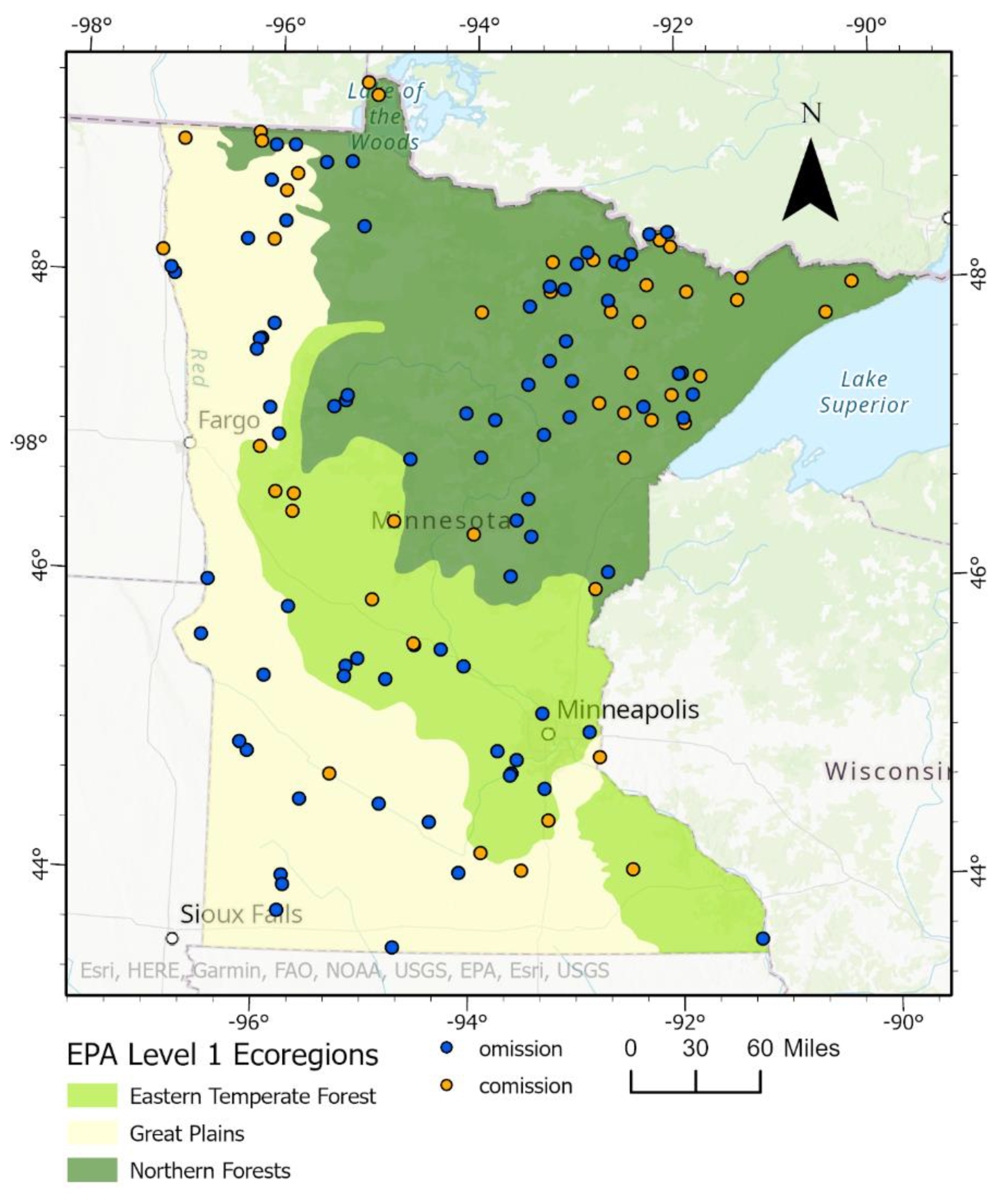
2.5. Quantitative Accuracy Assessment

The results of the model-fitting process were quantitatively assessed by manual interpretation of independent satellite imagery. To cover approximately the same time period as the harmonized Landsat–Sentinel time series, a set of images from the SPOT satellite series [54] were interpreted. SPOT1 coverage of Minnesota was fewer than 10 images with the majority of their area within the state. As such, to still include some assessment for the earliest part of the time series, all SPOT1 images with the majority of their area overlapping the state were interpreted. For the remainder of the SPOT archive, 25 images were selected for each of the following five-year periods over the time series: 1990–1994, 1995–1999, 2004–2009, and 2010–2014. The 25 images for each time period were selected to cover a randomly generated spatial location in the state. To meet selection criteria, images had to be captured within the same 5/1–6/30 time period as the harmonized Landsat-Sentinel time series, and have no more than 15% cloud cover. Images were then prioritized for interpretation based on their overlap with the study area, and centrality to the spring period. This yielded an assessment time series of 113 SPOT images from 1986–2014. For each of these images, 50 random points were sampled and manually interpreted as inundated or not inundated in ArcGIS Pro using false color display. Points obscured by cloud or intersecting developed land-cover were removed, yielding a final total of 5160 validation points to compare against the LandTrendr model (Table 3).

3. Results

3.1. Quantitive Accuracy

The LandTrendr model was highly accurate at predicting surface water dynamics over time as compared with manually-interpreted, independent satellite imagery. Overall accuracy was very high, at 98% (Table 3), which was driven by correct identification of dry-land pixels that made up the majority of validation points. For the inundated class specifically, accuracy was still high, but with greater rates of omission compared to commission. The inundated class had a producer’s accuracy of 82% and a user’s accuracy of 88% (Table 3). Omission of surface water appeared to be higher in part due to the coarseness of satellite imagery used: small or very narrow wetlands were difficult to identify if their percentage of a 30 m pixel was too low to distinguish from dry land with healthy vegetation (which can have SWF values as high as 30%). Additionally, some omission appeared to be due to a temporal mismatch between the medoid value used by the model and the accuracy assessment imagery. For example, some areas of temporary flooding were visible in the reference imagery, but the same flooding was not captured in the set of images used to fit the model. Commission of surface water also appeared to be due to temporal mismatch between the model imagery and the accuracy assessment imagery. Additionally, in the Northern Forests ecoregion specifically, a noted issue of DSWE confusing dark coniferous vegetation with water [45,46] appeared to be carried through to commission errors in this part of the state. Despite these weaknesses, the overall kappa coefficient was 0.835, suggesting very good agreement between the model predictions and reference dataset.
Error points in comparison to the reference dataset showed two distinct spatial patterns: clustering within one ecoregion, and clustering by year. While the Northern Forests and Eastern Temperate Forest ecoregions did not have significantly different accuracies from one another and were comparable to the accuracies for the overall dataset (Table 4 and Table 5), the Great Plains ecoregion in the south and west had a lower performance identifying surface water (Table 6, Figure 5). Specifically, the Great Plains ecoregion had a significantly lower producer’s accuracy for the inundated class when compared to the Northern Forests and Eastern Temperate Forest ecoregion (Z-statistic of 2.651) [55]. However, the Great Plains ecoregion still had a high overall accuracy (98%), and a relatively high kappa coefficient (0.73), suggesting the model still had acceptable performance for this region. Besides patterns in the error points by ecoregions, error points also show significant clustering by year (Moran’s I value of 0.2654, z-score of 6.14) (Figure 6), which could indicate the influence of specific images used to generate the model values or used as independent reference in accuracy assessment.

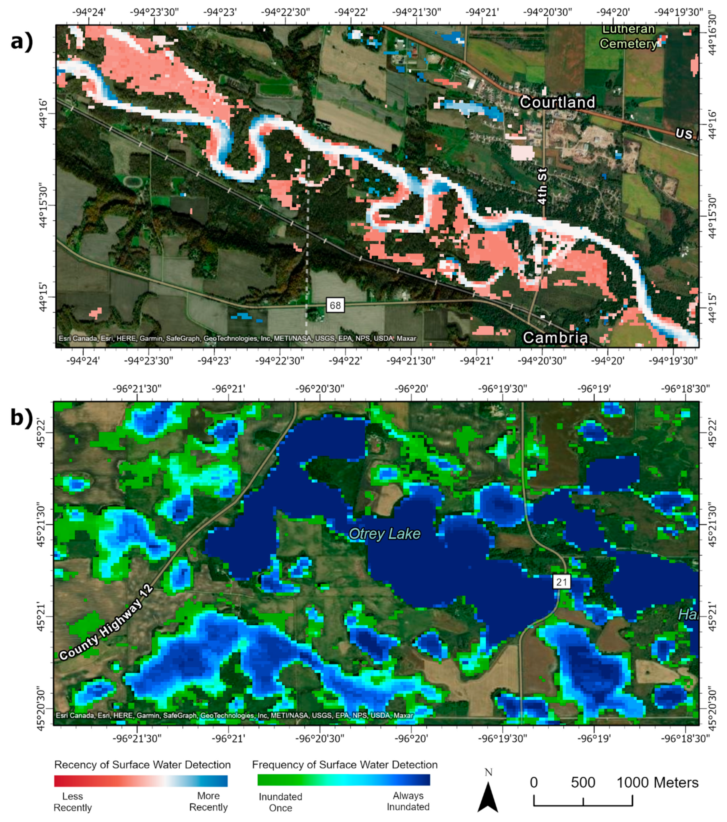
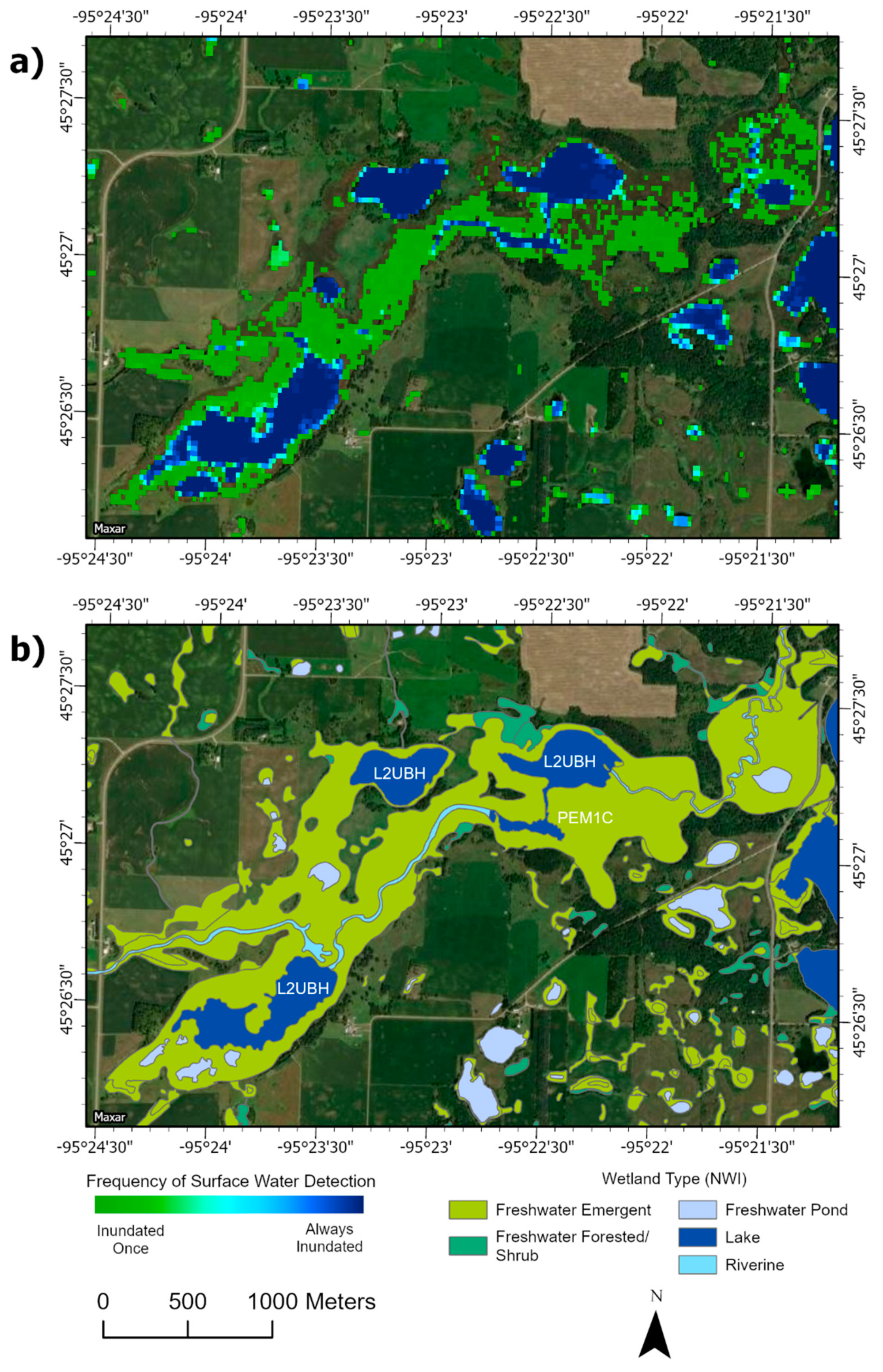
3.2. Qualitative Accuracy

At the pixel scale, LandTrendr correctly segmented the largest trends in surface water presence while removing noise (Figure 7). Using Figure 7b as an example, small interannual variations in SWF from 1984 to 1993 are modeled as a stable trendline of low surface water presence. However, larger trends, such as significant increases in water presence in 1996 and 2011 are reflected in the trendline, which correspond to years this location had higher than average precipitation in the spring. Further, a period of lower or decreasing surface water presence from 1984 to 1989 is commonly observed in the trendlines of pixels statewide, which corresponds to a severe, multi-year drought for much of the state. This suggests that the model can remove small, insignificant variations in SWF over the time series without removing change significant to wetland function. This segmentation also appeared consistently accurate across wetland types. Comparing the segmentation result to the original SWF values over time for different locations shows that LandTrendr removed noise equally well, despite differences in the expected degree of change over time. For example, trends in partial inundation for a peatland, which are small changes numerically, are identified as significant as well as transitions from dry to open water for a prairie pothole (Figure 7). This suggests that the segmentation can effectively scale with the amount of variability in the system, producing accurate long-term trends for wetlands with subtle to significant variability.
Aggregating the model results across multiple pixels more clearly illustrates that the model can effectively capture surface water conditions across wetland types. Maps of large-scale spatiotemporal inundation showed the expected patterns, including expansion and contraction of prairie pothole wetlands with climate trends, meandering of large rivers, and wetland conversion (Figure 8). Even in more stable locations, the model produces reasonable outputs at the multi-pixel scale: all water bodies showed a core area of persistent inundation ringed with pixels of less frequent inundation, illustrating that the model can identify maximum surface water extent. However, for palustrine emergent wetlands or ephemeral wetlands, the model produced a less reliable result (Figure 9). Regardless of actual inundation frequency, the model predicted them as very infrequently inundated (<5 years out of the past 35), suggesting that the model only identified those locations as having distinguishable surface water in a few extreme years. This results in patchy predictions of emergent wetlands, where small groups of pixels or the edges of the wetland are not identified. Despite this, locations that are predicted as inundated in multi-pixel aggregations show agreement with existing datasets. The distribution of inundation frequency predicted by LandTrendr for 4000 sample points are significantly different when separated by water regime classes according to the NWI (Kruskal–Wallis test p-value: 2.2 × 10⁻¹⁶), (Figure 10).

4. Discussion

4.1. Strengths and Limitations

While the accuracy achieved in this study shows that LandTrendr has promise for wetland monitoring, the errors observed suggest that there is also opportunity to improve results with further development.
Perhaps the greatest strength of LandTrendr for modeling surface water dynamics is its potential to accurately remove inter-annual noise from predictions of surface water presence. Wetlands are challenging to model from spectral information at a single timestep, given the high degree of heterogeneity in wetlands and mixed pixels containing spectral signatures for both water and vegetation [17]. Adding an additional temporal dimension to wetland modeling increases this difficulty, as small variations in the sample of images used in modeling each year may be misinterpreted as change. However, by regressing the expected values between inflection years, LandTrendr removes spurious noise predictions over time by evaluating a given year’s value within its temporal context. This ability to separate significant change from noise will be increasingly important as methods of long-term modeling improve with cloud computing, and climate change affects inter-annual climate patterns. Before tools like Google Earth Engine became available, performance of such long time series analysis was limited: requiring terabytes of data storage space and computing time on the order of weeks or months [15]. However, the comparable time series analysis performed here required no local storage space and could be run in a matter of days. This marked advancement in the ease with which large-scale temporal analysis can be performed will enable modeling of increasingly longer time series as the amount of available remote sensing data increases [56,57]. As time series grow in length and types of data, this ability to normalize predictions for a single year to follow patterns from a larger set of data will become more important to drawing conclusions from larger time series. Removing noise from the time series is also likely to be important as climate change increases the variability in Earth observations. Like many locations, Minnesota’s climate is expected to become more variable with climate change. While the state on the whole is predicted to have the same or greater total annual precipitation, the timing and intensity will shift to periods of intense precipitation with longer droughts between [58]. As the timing of precipitation becomes more variable with climate change, it is likely that inter-annual variations in weather will become an increasingly significant contributor to modeling noise. LandTrendr can compensate for this noise by removing many of the short-term fluctuations in its fitted trendlines, but still capture more significant climate related trends, as seen with the common identification of a multi-year drought in the 1980s.
The modeled trendlines produced by LandTrendr show reasonable patterns at the individual and multi-pixel scale for wetland monitoring, but are likely limited by the annual composites used. The surface reflectance images from Landsat and Sentinel-2 used to calculate annual composites of SWF values were chosen to represent the medoid surface water presence in the early spring (1 May to 30 June) each year. This date range was selected to capture normal high-water amounts in wetlands with the spring thaw while minimizing leaf cover. Choosing such a narrow window in an attempt to limit within-year variability seemingly contributed to much of the error, given the observed spatial clustering of errors (Figure 5 and Figure 6). The clustering of error points by year (Figure 6) suggests that error points tend to be located in the same images, so certain images or sets of images used in the model fitting were less accurate than others. This could be due to sparser parts of the larger time series: while using a harmonized Landsat and Sentinel-2 dataset meant many locations had multiple images in a given year, other locations had only one or two images due to a high number of cloudy or otherwise erroneous images. These sparse samples may not necessarily provide an accurate representation of that location’s spring condition. For example, cloud presence over a location in a given year may skew the composited observations earlier or later within that year, missing normal periods of inundation. As prairie potholes are especially variable in surface water presence inter- and intra-annually, differences in a given year’s image sample could also help explain the spatial clustering of errors in this region due to missing peak inundation (Figure 5). To correct this, more information on the status of a wetland in a given year can be created by applying LandTrendr to different annual composites than those created here from this narrow spring window. Interesting future work could include using maximum or minimum SWF values within a period to intentionally capture more extreme ends of surface water presence over time, using a longer temporal window so that a location tends to have more observations, or including additional time periods to the training data in the SWF algorithm such as mid-summer or fall conditions.
Similarly, while applying the SWF algorithm with the LandTrendr parameters here produced good results for a variety of wetlands, the model could be modified to further enhance the final trendlines predicted by LandTrendr. A key benefit of using SWF as the variable monitored by LandTrendr is its ability to approximate subtle changes in relative surface water and vegetation presence, similar to SMA [17,25]. While the results suggest potential to accurately model partial surface water presence (e.g., showing reasonable partial water presence for bogs, Figure 7a), performance for emergent wetlands more generally appears to underestimate surface water presence. This produces a patchy appearance where small groups of pixels or the edges of the wetland are not identified. Thus, while aggregations of the model output, such as the frequency of inundation in the past 35 years, can approximate wetland locations, temporal trends are more difficult to interpret and it is likely many of these types of wetland are never detected as inundated, contributing to omission. (Figure 9). The algorithm also creates many small patches of commission for ~50–70% inundation that appear infrequently in the time series, creating a signature easily confused with emergent wetlands. While LandTrendr is intended to handle some degree of noise in the annual composites, it appears that some of these errors in the SWF composites can be interpreted as significant under certain LandTrendr parameter settings. A clear example of this is in Figure 7a, where a significant drop is identified in SWF after 1999 that looks indistinguishable from other drops in SWF smoothed out as noise elsewhere. As the LandTrendr parameters chosen here were optimized based on state-wide metrics, their interaction with the interannual noise characteristics for this specific pixel or specific system could be producing a spurious trendline. Further, because SWF values at the beginning or end of the time series are not normalized as in other parts of the time series, errors here can be especially influential. In the LandTrendr algorithm, the first and final years serve as anchors for the larger segmentation. As such, an erroneous SWF value at the start or end of the time series is treated as an inflection point regardless of whether it would be treated as noise elsewhere, thereby skewing the trendline. Thus, there appears to be a limit to how much model noise for which LandTrendr can compensate, and careful development is required for both the metric to segment and how it will be segmented.
SWF could be improved in this application by modifying the development of training data and the LandTrendr parameters used with it. The SWF algorithm trains a random forest model to identify partial water presence by coarsening the resolution of a water presence/absence map derived from DSWE. As such, training data for partial surface water values represent only partial surface water conditions derived from the edge of fully inundated features, and does not explicitly capture partial inundation from emergent vegetation. While this would make LandTrendr less automated and generalizable than described here, including training points for emergent vegetation from alternate data or manual interpretation could also improve performance. Second, additional constraints to DSWE could limit its contribution of noise to the SWF time series. DSWE is a set of spectral tests to identify surface water that has been shown to be robust to a wide variety of wetland types, but with a known tendency for confusion with land cover types like dark vegetation and omission of some emergent vegetation [20]. These weaknesses are especially pronounced in parts of the state where the sample of surface reflectance images in a year was smaller, as described previously. Such locations either had spurious regions of lower confidence wetland according to DSWE or omitted large areas of emergent wetland. Other papers using DSWE have modified the spectral tests used to identify surface water to account for these issues, which may also improve results in this case. For example, Vanderhoof et al. added an additional test to more conservatively predict surface water while applying DSWE to identify anthropogenic wetland disturbance [16]. Using similarly stringent rules for this application, such as treating lower confidence predictions of water presence from DSWE as water absence, could improve the performance of the random forest model trained with it. Additionally, using more conservative estimates of surface water presence the key years at the start and end of the time series may also improve overall results by accounting for the influence these years have on the rest of the trendline. Finally, a more tailored parameterization of LandTrendr than the statewide example tested here could improve results. While the parameterization here suggests LandTrendr can successfully be applied over large and diverse systems, parameterizing specifically for SWF values observed in smaller areas or wetland types may enable more accurate trendlines at small scales.

4.2. Potential Applications

The level of detail and accuracy of the LandTrendr output suggests it has greatest potential as a temporal complement to existing datasets. Given the difficulty of producing similar enough trendlines across neighboring pixels to produce contiguous wetland objects (Figure 9), commission of partial inundation conditions, and omission emergent wetlands, it is unlikely LandTrendr will be able to fully replace existing wetland inventory efforts or the in situ estimates of change provided by on-the-ground monitoring programs. However, the annual information produced for every 30 m pixel in the state can help fill in temporal information that would be missed by other methods. In particular, LandTrendr seems especially suited to maintaining the accuracy of the NWI over time. While the NWI provides highly detailed classification information at high spatial detail (0.5 ha), it achieves such high accuracy by being based partially on manual interpretation [59]. Methods of automation have been developed, but the inventory is still a time-consuming and expensive process, with nearly 30 years between the original and updated inventories for the state [59]. This lag in updates for the NWI has real consequences for its effectiveness as a management tool. Estimates by Oslund et al. more than a decade before the updated wetlands inventory found that as much as 4% of wetlands area in the Prairie Pothole Region were no longer accurate in the NWI at that time [60]. By identifying only the most significant changes in a pixel’s temporal context annually, LandTrendr could indicate locations in the NWI that have changed, enabling the update process to occur more frequently at a localized scale. Potential for this use is evident in comparison of the LandTrendr result to the NWI (Figure 10). The LandTrendr result can separate water regime class as specified in the NWI (Figure 10). This separability suggests that changes in frequency of inundation or other LandTrendr-derived metrics could signify changes to water regime that would require re-inventorying for that location.

5. Conclusions

Successful management of wetlands now and in the future will require frequent monitoring and an understanding of how conditions fit within that location’s larger temporal context. Here we explore the temporal segmentation algorithm LandTrendr for this purpose by applying LandTrendr to surface water dynamics in Minnesota from 1984 to 2019. This model was very accurate in comparison to an independent set of image interpretations. Qualitatively, these results also appear accurate at multiple scales. Surface water trendlines for individual pixels were as expected for a variety of wetland types and degrees of inundation, removing spurious interannual fluctuations in values but identifying longer-term trends. Aggregations of trendlines across multiple pixels also produced reasonable trends spatially and temporally, and can create larger maps of landscape-level surface water dynamics such as frequency or recency of inundation. The high accuracies achieved here suggest that LandTrendr could be a valuable tool for increasing the confidence of long, complex time series analysis, and already shows the ability to identify changes in the NWI by being able to separate water regime classes. These high accuracies were achieved with relatively minimal input: optimal parameters for LandTrendr in this system were identified, but the SWF algorithm used with LandTrendr requires no training data outside of the time series of surface reflectance images, suggesting it could be easily applied to monitor wetlands generally. However, spatial clustering of error locations and relatively poor performance identifying areas of emergent wetlands suggest that performance is strongly influenced by the time series provided, and there is a limit to the amount of noise in the time-series for which LandTrendr can compensate. The methods described here are intended to minimize the amount of training to evaluate LandTrendr’s performance generally, but including additional training data to more accurately capture inundation for different wetlands or varying parameterizations by wetland type or location could further enhance the accuracy of LandTrendr results. Overall, the accuracy achieved here in this initial application suggests LandTrendr is suitable for wetland monitoring from the local to regional scale.

Supplementary Materials

The following supporting information can be downloaded at: https://www.mdpi.com/article/10.3390/rs14112662/s1, Supplementary Materials Section S1: Number of images contributing to the time series; Supplementary Materials Section S2: Parameter selection for the LandTrendr algorithm.

Author Contributions

Conceptualization, J.F.K.; methodology, A.C.L.; software, A.C.L.; validation, A.C.L.; formal analysis, A.C.L.; investigation, A.C.L.; resources, J.F.K.; data curation, A.C.L.; writing—original draft preparation, A.C.L.; writing—review and editing, J.F.K. and A.C.L.; visualization, A.C.L.; supervision, J.F.K.; project administration, J.F.K.; funding acquisition, J.F.K. All authors have read and agreed to the published version of the manuscript.

Funding

This research was funded by the EPA Region 5 Wetland Program Development Grant program, grant number CD-00E02740-0.

Data Availability Statement

Data available on request of corresponding author.

Acknowledgments

We thank Jody Vogeler and Mitchell Bonney for guidance in fitting LandTrendr, as well as Jennie Skancke and Steve Kloiber for stakeholder input during model development.

Conflicts of Interest

The authors declare no conflict of interest.

References

  1. Dahl, T.E. Wetlands Losses in the United States 1780′s to 1980′s; US Department of the Interior, Fish and Wildlife Service: Washington, DC, USA, 1990; Volume 13.
  2. Dahl, T.E. Status and Trends of Wetlands in the Conterminous United States 2004 to 2009; US Department of the Interior, Fish and Wildlife Service: Washington, DC, USA, 2009.
  3. Dahl, T.E. Status and Trends of Prairie Wetlands in the United States 1997 to 2009; U.S. Department of the Interior, Fish and Wildlife Service, Ecological Services: Washington, DC, USA, 2014.
  4. Saunders, S.P.; Hall, K.A.L.; Hill, N.; Michel, N.L. Multiscale Effects of Wetland Availability and Matrix Composition on Wetland Breeding Birds in Minnesota, USA. Condor Ornithol. Appl. 2019, 59, 1–15. [Google Scholar] [CrossRef]
  5. Cheng, F.Y.; Van Meter, K.J.; Byrnes, D.K.; Basu, N.B. Maximizing US Nitrate Removal through Wetland Protection and Restoration. Nature 2020, 588, 625–630. [Google Scholar] [CrossRef] [PubMed]
  6. Hansen, A.T.; Dolph, C.L.; Foufoula-Georgiou, E.; Finlay, J.C. Contribution of Wetlands to Nitrate Removal at the Watershed Scale. Nat. Geosci. 2018, 11, 127–132. [Google Scholar] [CrossRef]
  7. Goldberg, N.; Reiss, K.C. Accounting for Wetland Loss: Wetland Mitigation Trends in Northeast Florida 2006–2013. Wetlands 2016, 36, 373–384. [Google Scholar] [CrossRef]
  8. Fickas, K.C.; Cohen, W.B. Landsat-Based Monitoring of Annual Wetland Change in the Willamette Valley of Oregon, USA from 1972 to 2012. Wetl. Ecol. Manag. 2016, 24, 73–92. [Google Scholar] [CrossRef]
  9. Bendor, T. Landscape and Urban Planning A Dynamic Analysis of the Wetland Mitigation Process and Its Effects on No Net Loss Policy. Landsc. Urban Plan. 2009, 89, 17–27. [Google Scholar] [CrossRef]
  10. Kloiber, S.M.; Norris, D.J. Monitoring Changes in Minnesota Wetland Area and Type from 2006 to 2014. Wetl. Sci. Pract. 2017, 34, 76–87. [Google Scholar]
  11. Green, A.J.; Alcorlo, P.; Morris, E.P. Creating a Safe Operating Space for Wetlands in a Changing Climate. Front. Ecol. Environ. 2017, 15, 99–107. [Google Scholar] [CrossRef] [Green Version]
  12. Beier, C.; Briske, D.D.; Classen, A.T.; Luo, Y.; Reichstein, M.; Smith, M.D.; Smith, S.D.; Bell, J.E.; Fay, P.A.; Heisler, J.L.; et al. Consequences of More Extreme Precipitation Regimes for Terrestrial Ecosystems. Bioscience 2008, 58, 811–821. [Google Scholar]
  13. Zhang, Z.; Lei, L.; He, Z.; Su, Y.; Li, L.; Wang, X.; Guo, X. Tracking Changing Evidences of Water in Wetland Using the Satellite Long-Term Observations from 1984 to 2017. Water 2020, 12, 1602. [Google Scholar] [CrossRef]
  14. Krause, C.E.; Newey, V.; Alger, M.J.; Lymburner, L. Mapping and Monitoring the Multi-Decadal Dynamics of Australia’s Open Waterbodies Using Landsat. Remote Sens. 2021, 13, 1437. [Google Scholar] [CrossRef]
  15. Carroll, M.; Wooten, M.; DiMiceli, C.; Sohlberg, R.; Kelly, M. Quantifying Surface Water Dynamics at 30 Meter Spatial Resolution in the North American High Northern Latitudes 1991–2011. Remote Sens. 2016, 8, 622. [Google Scholar] [CrossRef] [Green Version]
  16. Vanderhoof, M.K.; Christensen, J.; Beal, Y.J.G.; DeVries, B.; Lang, M.W.; Hwang, N.; Mazzarella, C.; Jones, J.W. Isolating Anthropogenic Wetland Loss by Concurrently Tracking Inundation and Land Cover Disturbance across the Mid-Atlantic Region, U.S. Remote Sens. 2020, 12, 1464. [Google Scholar] [CrossRef] [PubMed]
  17. Halabisky, M.; Moskal, L.M.; Gillespie, A.; Hannam, M. Reconstructing Semi-Arid Wetland Surface Water Dynamics through Spectral Mixture Analysis of a Time Series of Landsat Satellite Images (1984–2011). Remote Sens. Environ. 2016, 177, 171–183. [Google Scholar] [CrossRef]
  18. Adeli, S.; Salehi, B.; Mahdianpari, M.; Quackenbush, L.J.; Brisco, B.; Tamiminia, H.; Shaw, S. Wetland Monitoring Using SAR Data: A Meta-Analysis and Comprehensive Review. Remote Sens. 2020, 12, 2190. [Google Scholar] [CrossRef]
  19. Che, X.; Feng, M.; Sexton, J.; Channan, S.; Sun, Q.; Ying, Q.; Liu, J.; Wang, Y. Landsat-Based Estimation of Seasonal Water Cover and Change in Arid and Semi-Arid Central Asia (2000–2015). Remote Sens. 2019, 11, 1323. [Google Scholar] [CrossRef] [Green Version]
  20. Jones, J.W. Efficient Wetland Surface Water Detection and Monitoring via Landsat: Comparison with in Situ Data from the Everglades Depth Estimation Network. Remote Sens. 2015, 7, 12503–12538. [Google Scholar] [CrossRef] [Green Version]
  21. Mahdianpari, M.; Jafarzadeh, H.; Granger, J.E.; Mohammadimanesh, F.; Salehi, B.; Homayouni, S.; Weng, Q.; Jafarzadeh, H.; Granger, J.E.; Mohammadimanesh, F. A Large-Scale Change Monitoring of Wetlands Using Time Series Landsat Imagery on Google Earth Engine: A Case Study in Newfoundland. GISci. Remote Sens. 2020, 57, 1102–1124. [Google Scholar] [CrossRef]
  22. Wulder, M.A.; Li, Z.; Campbell, E.M.; White, J.C.; Hobart, G.; Hermosilla, T.; Coops, N.C. A National Assessment Ofwetland Status and Trends for Canada’s Forested Ecosystems Using 33 Years of Earth Observation Satellite Data. Remote Sens. 2018, 10, 1623. [Google Scholar] [CrossRef] [Green Version]
  23. Sall, I.; Jarchow, C.J.; Sigafus, B.H.; Eby, L.A.; Forzley, M.J.; Hossack, B.R. Estimating Inundation of Small Waterbodies with Sub-Pixel Analysis of Landsat Imagery: Long-Term Trends in Surface Water Area and Evaluation of Common Drought Indices. Remote Sens. Ecol. Conserv. 2021, 7, 109–124. [Google Scholar] [CrossRef]
  24. Kayastha, N.; Thomas, V.; Galbraith, J.; Banskota, A. Monitoring Wetland Change Using Inter-Annual Landsat Time-Series Data. Wetlands 2012, 32, 1149–1162. [Google Scholar] [CrossRef]
  25. Halabisky, M.; Babcock, C.; Moskal, L.M. Harnessing the Temporal Dimension to Improve Object-Based Image Analysis Classification of Wetlands. Remote Sens. 2018, 10, 1467. [Google Scholar] [CrossRef] [Green Version]
  26. Kennedy, R.E.; Yang, Z.; Cohen, W.B. Detecting Trends in Forest Disturbance and Recovery Using Yearly Landsat Time Series: 1. LandTrendr—Temporal Segmentation Algorithms. Remote Sens. Environ. 2010, 114, 2897–2910. [Google Scholar] [CrossRef]
  27. Kennedy, R.E.; Yang, Z.; Gorelick, N.; Braaten, J.; Cavalcante, L.; Cohen, W.B.; Healey, S. Implementation of the LandTrendr Algorithm on Google Earth Engine. Remote Sens. 2018, 10, 691. [Google Scholar] [CrossRef] [Green Version]
  28. Bonney, M.T.; He, Y.; Myint, S.W. Contextualizing the 2019–2020 Kangaroo Island Bushfires: Quantifying Landscape-Level Influences on Past Severity and Recovery with Landsat and Google Earth Engine. Remote Sens. 2020, 12, 3942. [Google Scholar] [CrossRef]
  29. Vogeler, J.C.; Braaten, J.D.; Slesak, R.A.; Falkowski, M.J. Extracting the Full Value of the Landsat Archive: Inter-Sensor Harmonization for the Mapping of Minnesota Forest Canopy Cover (1973–2015). Remote Sens. Environ. 2018, 209, 363–374. [Google Scholar] [CrossRef]
  30. Ye, L.; Liu, M.; Liu, X.; Zhu, L. Developing a New Disturbance Index for Tracking Gradual Change of Forest Ecosystems in the Hilly Red Soil Region of Southern China Using Dense Landsat Time Series. Ecol. Inform. 2021, 61, 101221. [Google Scholar] [CrossRef]
  31. Long, X.; Li, X.; Lin, H.; Zhang, M. Mapping the Vegetation Distribution and Dynamics of a Wetland Using Adaptive-Stacking and Google Earth Engine Based on Multi-Source Remote Sensing Data. Int. J. Appl. Earth Obs. Geoinf. 2021, 102, 102453. [Google Scholar] [CrossRef]
  32. Chai, X.R.; Li, M.; Wang, G.W. Characterizing Surface Water Changes across the Tibetan Plateau Based on Landsat Time Series and LandTrendr Algorithm. Eur. J. Remote Sens. 2022, 55, 251–262. [Google Scholar] [CrossRef]
  33. Braaten, J.D.; Kennedy, R.E. LT-GEE Guide. Available online: https://emapr.github.io/LT-GEE/ (accessed on 24 May 2022).
  34. Kloiber, S.M. Status and Trends of Wetlands in Minnesota: Wetland Quantity Baseline; Department of Natural Resources: St. Paul, MN, USA, 2010; p. 28.
  35. Leibowitz, S.G.; Mushet, D.M.; Newton, W.E. Intermittent Surface Water Connectivity: Fill and Spill vs. Fill and Merge Dynamics. Wetlands 2016, 36, 323–342. [Google Scholar] [CrossRef]
  36. Vanderhoof, M.K.; Alexander, L.C. The Role of Lake Expansion in Altering the Wetland Landscape of the Prairie Pothole Region, United States. Wetlands 2016, 36, 309–321. [Google Scholar] [CrossRef] [PubMed] [Green Version]
  37. Wulder, M.A.; White, J.C.; Loveland, T.R.; Woodcock, C.E.; Belward, A.S.; Cohen, W.B.; Fosnight, E.A.; Shaw, J.; Masek, J.G.; Roy, D.P. The Global Landsat Archive: Status, Consolidation, and Direction. Remote Sens. Environ. 2016, 185, 271–283. [Google Scholar] [CrossRef] [Green Version]
  38. Drusch, M.; Del Bello, U.; Carlier, S.; Colin, O.; Fernandez, V.; Gascon, F.; Hoersch, B.; Isola, C.; Laberinti, P.; Martimort, P.; et al. Sentinel-2: ESA’s Optical High-Resolution Mission for GMES Operational Services. Remote Sens. Environ. 2012, 120, 25–36. [Google Scholar] [CrossRef]
  39. Runge, A.; Grosse, G. Mosaicking Landsat and Sentinel-2 Data to Enhance LandTrendr Time Series Analysis in Northern High Latitude Permafrost Regions. Remote Sens. 2020, 12, 2471. [Google Scholar] [CrossRef]
  40. Claverie, M.; Ju, J.; Masek, J.G.; Dungan, J.L.; Vermote, E.F.; Roger, J.C.; Skakun, S.V.; Justice, C. The Harmonized Landsat and Sentinel-2 Surface Reflectance Data Set. Remote Sens. Environ. 2018, 219, 145–161. [Google Scholar] [CrossRef]
  41. Nguyen, M.D.; Baez-Villanueva, O.M.; Bui, D.D.; Nguyen, P.T.; Ribbe, L. Harmonization of Landsat and Sentinel 2 for Crop Monitoring in Drought Prone Areas: Case Studies of Ninh Thuan (Vietnam) and Bekaa (Lebanon). Remote Sens. 2020, 12, 281. [Google Scholar] [CrossRef] [Green Version]
  42. Poortinga, A.; Tenneson, K.; Shapiro, A.; Nquyen, Q.; Aung, K.S.; Chishtie, F.; Saah, D. Mapping Plantations in Myanmar by Fusing Landsat-8, Sentinel-2 and Sentinel-1 Data along with Systematic Error Quantification. Remote Sens. 2019, 11, 831. [Google Scholar] [CrossRef] [Green Version]
  43. Roy, D.P.; Kovalskyy, V.; Zhang, H.K.; Vermote, E.F.; Yan, L.; Kumar, S.S.; Egorov, A. Characterization of Landsat-7 to Landsat-8 Reflective Wavelength and Normalized Difference Vegetation Index Continuity. Remote Sens. Environ. 2016, 185, 57–70. [Google Scholar] [CrossRef] [Green Version]
  44. Rampi, L.P.; Knight, J.F.; Bauer, M. Minnesota Land Cover Classification and Impervious Surface Area by Landsat and Lidar: 2013-14 Update; University of Minnesota: Minneapolis, MN, USA, 2016. [Google Scholar] [CrossRef]
  45. De Vries, B.; Huang, C.; Lang, M.W.; Jones, J.W.; Huang, W.; Creed, I.F.; Carroll, M.L. Automated Quantification of Surface Water Inundation in Wetlands Using Optical Satellite Imagery. Remote Sens. 2017, 9, 807. [Google Scholar] [CrossRef] [Green Version]
  46. Jones, J.W. Improved Automated Detection of Subpixel-Scale Inundation-Revised Dynamic Surface Water Extent (DSWE) Partial Surface Water Tests. Remote Sens. 2019, 11, 374. [Google Scholar] [CrossRef] [Green Version]
  47. Wilson, J.P.; Gallant, J.C. Terrain Analysis: Principles and Applications; John Wiley & Sons: Hoboken, NJ, USA, 2000. [Google Scholar]
  48. Lehner, B.; Verdin, K.; Jarvis, A. New Global Hydrography Derived from Spaceborne Elevation Data. Eos Trans. Am. Geophys. Union 2008, 89, 93–94. [Google Scholar] [CrossRef]
  49. Boulesteix, A.-L.; Janitza, S.; Kruppa, J.; König, I.R. Overview of Random Forest Methodology and Practical Guidance with Emphasis on Computational Biology and Bioinformatics. WIREs Data Min. Knowl. Discov. 2012, 2, 493–507. [Google Scholar] [CrossRef] [Green Version]
  50. Crist, E.P. A TM Tasseled Cap Equivalent Transformation for Reflectance Factor Data. Remote Sens. Environ. 1985, 17, 301–306. [Google Scholar] [CrossRef]
  51. McFeeters, S.K. The Use of the Normalized Difference Water Index (NDWI) in the Delineation of Open Water Features. Int. J. Remote Sens. 1996, 17, 1425–1432. [Google Scholar] [CrossRef]
  52. Xu, H. Modification of Normalised Difference Water Index (NDWI) to Enhance Open Water Features in Remotely Sensed Imagery. Int. J. Remote Sens. 2006, 27, 3025–3033. [Google Scholar] [CrossRef]
  53. Tucker, C.J. Red and Photographic Infrared Linear Combinations for Monitoring Vegetation. Remote Sens. Environ. 1979, 8, 127–150. [Google Scholar] [CrossRef] [Green Version]
  54. Arnaud, M. The SPOT Program—Status of the Current Satellites and the Future. In Proceedings of the Euro-Asian Space Week—Co-Operation in Space: Where East & West Finally Meet, Singapore, 23–27 November 1998; European Space Agency: Paris, France, 1999; Volume 430, pp. 369–376. [Google Scholar]
  55. Congalton, R.G.; Green, K. Assessing the Accuracy of Remotely Sensed Data, Principles and Practices; CRC Press: Boca Raton, FL, USA, 2019. [Google Scholar]
  56. Masek, J.G.; Wulder, M.A.; Markham, B.; McCorkel, J.; Crawford, C.J.; Storey, J.; Jenstrom, D.T. Landsat 9: Empowering Open Science and Applications through Continuity. Remote Sens. Environ. 2020, 248, 111968. [Google Scholar] [CrossRef]
  57. Gorelick, N.; Hancher, M.; Dixon, M.; Ilyushchenko, S.; Thau, D.; Moore, R. Google Earth Engine: Planetary-Scale Geospatial Analysis for Everyone. Remote Sens. Environ. 2017, 202, 18–27. [Google Scholar] [CrossRef]
  58. Noe, R.R.; Keeler, B.L.; Twine, T.E.; Brauman, K.A.; Mayer, T.; Rogers, M. Climate Change Projections for Improved Management of Infrastructure, Industry, and Water Resources in Minnesota. University of Minnesota Digital Conservancy. 2019. Available online: https://hdl.handle.net/11299/209130 (accessed on 24 May 2022).
  59. Kloiber, S.M.; Macleod, R.D.; Smith, A.J.; Knight, J.F.; Huberty, B.J. A Semi-Automated, Multi-Source Data Fusion Update of a Wetland Inventory for East-Central Minnesota, USA. Wetlands 2015, 35, 335–348. [Google Scholar] [CrossRef]
  60. Oslund, F.T.; Johnson, R.R.; Hertel, D.R. Assessing Wetland Changes in the Prairie Pothole Region of Minnesota from 1980 to 2007. J. Fish Wildl. Manag. 2010, 1, 131–135. [Google Scholar] [CrossRef]
Figure 1. Conceptual diagram of the LandTrendr algorithm (adapted from Kennedy et al. [26,27,33]). Given a time series of surface reflectance information (represented in green), LandTrendr will segment the changes in pixel-values for a location over time (represented in blue). The result is a set of key inflection years and a linear regression between them (represented in black).
Remotesensing 14 02662 g001
Figure 2. Ecoregions of Minnesota and their wetland types. Minnesota contains 10.6 million acres of wetland in three different ecoregions according to EPA Level 1 designations [34]. The north is dominated by coniferous forest and peatland, the central and southeast contain mixed deciduous forest with forested wetlands and lakes, and the south and west contain cultivated prairie and depressional prairie pothole wetlands.
Remotesensing 14 02662 g002
Figure 3. Area of land cover classes in Minnesota by ecoregion from the 2013–2014 land cover and impervious surface dataset for Minnesota [44]. All three of the EPA Level 1 Ecoregions in Minnesota contain significant areas of wetlands to identify, but their landscape contexts are very different. The Eastern Temperate Forests ecoregion contains a relatively even mixture of wetland, agriculture, forest, and grass. The Great Plains ecoregion contains the lowest absolute area of wetlands as many have been drained for the large area of agricultural cultivation in the region. The Northern Forests ecoregion contains the greatest area of wetlands and open water, but is also highly forested, which complicates the detection of wetlands from satellite imagery.
Remotesensing 14 02662 g003
Figure 4. The SWF algorithm (adapted from De Vries et al. [45]). The percent surface water coverage of a pixel is produced at the 30 m scale using a self-trained random forest model of 500 trees. The random forest model is trained using a set of spectral indices and raw band values from harmonized Landsat and Sentinel data rescaled to the 150 m resolution (the training data), and DSWE reclassified to binary surface water presence/absence rescaled to the 150 m resolution (the predicted variable).
Remotesensing 14 02662 g004
Figure 5. The spatial distribution of accuracy assessment errors. The Northern Forests and Eastern Temperate Forest ecoregions have similar amounts of omission and commission points, with similar accuracies to the overall accuracy. The Great Plains ecoregion has a disproportionately high number of omission points, leading to a significantly lower producer’s accuracy for this region.
Remotesensing 14 02662 g005
Figure 6. The temporal distribution of accuracy assessment errors. Error points show significant clustering by year (Moran’s I value of 0.2654, z-score of 6.14). This suggests that individual images in either the model development process or the independent reference set have a clear influence on errors in the model.
Remotesensing 14 02662 g006
Figure 7. Examples of the LandTrendr fit for individual pixels. LandTrendr produces consistent temporal segmentations across different wetland types and expected variability of the system. Small fluctuations in surface water amount from year to year are removed, whereas long-term trends over time are identified. (a) LandTrendr fit for a peatland at the edge of Red Lake. Despite the fact that changes in this wetland are relatively small over time (ranging from 30–60% SWF), it still identifies a general trend of higher values around 1998. It also identifies a drop in values in 1999, which may not be significant in the larger context. (b) LandTrendr fit for the edge of a large prairie pothole near Big Stone Lake. LandTrendr effectively models extreme changes from dry (in the 1980s and 2000s) to periods with near-total inundation due to high precipitation (the late 1990s and early 2010s). (c) LandTrendr fit for the Minnesota River near St. Peter. Despite a high degree of variability in the early 1990s, LandTrendr can identify when this location became part of the main channel in the early 2000s, correctly identifying two key time periods at this location.
Remotesensing 14 02662 g007
Figure 8. Example multi-pixel aggregations of the LandTrendr result. (a) The LandTrendr result summarized to recency of inundation for the Minnesota River at Courtland. The model correctly identifies temporal changes in inundation over time, showing the river to be more-recently inundated at the outer edge where meanders are carving, and less-recently inundated on the inner edge where meanders are filled in. (b) The LandTrendr result summarized to frequency of inundation for a prairie pothole complex near Ortonville. The model correctly identifies the larger, deeper basins at the center of the image as being permanently inundated, while shallower surrounding basins that would dry out under drought conditions are semi-permanently inundated.
Remotesensing 14 02662 g008
Figure 9. The performance of LandTrendr for emergent wetlands as compared to the National Wetlands Inventory. (a) The LandTrendr result for an emergent wetland in western Minnesota, near Swift Falls. (b) The National Wetlands Inventory data for the same region. Note that while the persistently inundated deep-water basins in panel b have approximately the correct shape in panel a, the emergent wetlands surrounding them that are only seasonally inundated for short periods (PEM1C Cowardin classification) appear as infrequently inundated in panel a, with individual pixels and larger areas not predicted as inundated at all. There are also very small patches (<5 pixels) that are commission in the LandTrendr output but appear similar in frequency of inundation to emergent vegetation.
Remotesensing 14 02662 g009
Figure 10. The separability of NWI Water Regime class by percent of years inundated predicted by LandTrendr. A set of 4000 random points were sampled within the NWI for Minnesota, with 1000 points per water regime class. The distribution of percent of years inundated as predicted by LandTrendr is plotted by water regime class. Note that the different water regime classes have significantly different distributions of predicted frequency of inundation (Kruskal–Wallis test p-value: 2.2 × 10⁻¹⁶), suggesting that changes in LandTrendr predictions could be associated to changes in water regime class.
Remotesensing 14 02662 g010
Table 2. Parameter settings used for fitting LandTrendr (originally described by Kennedy et al. [26,27,33]. These settings were found to minimize omission of previously-identified surface water compared to the NWI. Values marked with an asterisk were not systematically varied to find the optimal setting, but were accepted at this value a priori based on the expected behavior of the system or performance of the model.
Parameter:Description:Value:
Maximum Segments (maxSegments)Maximum number of segments allowed in the fitted segmentation11
Spike Threshold (spikeThreshold)Threshold for dampening spikes (1.0 is no dampening)0.5
Vertex Count Overshoot
(vertexCountOvershoot)
The number of vertices by which the initial model can exceed the maximum
segments before pruning
2
Prevent One Year Recovery
(preventOneYearRecovery)
Whether to prevent segments that are a one-year recovery back to a previous levelFalse *
Recovery Threshold (recoveryThreshold)Segment slopes are limited to a rate of less than 1/Recovery Threshold0.25
p-value Threshold (pvalThreshold)Maximum p-value of the best model.0.1
Best Model Proportion
(bestModelProportion)
Defines the best model as that with the most vertices with a p-value that is at most this proportion away from the model with the lowest p-value1
Minimum Number of Observations Needed (minObsNeeded)Minimum number of observations in the time series for the model to fit.31 *
Table 3. The confusion matrix for the LandTrendr model statewide. The performance of the LandTrendr model when compared to manual interpretation of independent satellite imagery. Overall accuracy is high at 98%, producer’s and user’s accuracies for the inundated class are 82% and 88%, respectively. This suggests good performance of the LandTrendr model in identifying surface water.
ClassificationRow Total:
Dry:Inundated:
ReferenceDry:4685474732
Inundated:78350428
Column Total:4763397n = 5160
Inundated Producer’s Accuracy:82%
Inundated User’s Accuracy:88%
Overall Accuracy:98%
Kappa Coefficient:0.835
Table 4. The confusion matrix for the LandTrendr model in the Northern Forests Ecoregion. The performance of the LandTrendr model when compared to manual interpretation of independent satellite imagery in the Northern Forests ecoregion (northern and northeastern parts of the state). Overall accuracy is high at 97%, producer’s and user’s accuracies for the inundated class are 85% and 89%, respectively. This suggests good performance of the LandTrendr model, similar to the overall accuracy, in identifying surface water in this region.
Classification
(Northern Forests)
Row Total:
Dry:Inundated:
Reference
(Northern Forests)
Dry:1659281687
Inundated:38219257
Column Total:1697247n = 1944
Inundated Producer’s Accuracy:85%
Inundated User’s Accuracy:89%
Overall Accuracy:97%
Kappa Coefficient:0.850
Table 5. The confusion matrix for the LandTrendr model in the Eastern Temperate Forest Ecoregion. The performance of the LandTrendr model when compared to manual interpretation of independent satellite imagery in the Eastern Temperate Forest ecoregion (central and southeastern parts of the state). Overall accuracy is high at 98%, producer’s and user’s accuracies for the inundated class are 86% and 88%, respectively. This suggests good performance of the LandTrendr model, similar to the overall accuracy, in identifying surface water in this region.
Classification
(Eastern Temperate Forest)
Row Total:
Dry:Inundated:
Reference
(Eastern Temperate Forest)
Dry:1095111106
Inundated:148397
Column Total:110994n = 1203
Inundated Producer’s Accuracy:86%
Inundated User’s Accuracy:88%
Overall Accuracy:98%
Kappa Coefficient:0.858
Table 6. The confusion matrix for the LandTrendr model in the Great Plains Ecoregion. The performance of the LandTrendr model when compared to manual interpretation of independent satellite imagery in the Great Plains ecoregion (the western and southwestern parts of the state). Overall accuracy is still high at 98%, but the producer’s and user’s accuracies for the inundated class specifically are 65% and 86%, respectively. This suggests the model struggled with identifying surface water in this region more than elsewhere.
Classification
(Great Plains)
Row Total:
Dry:Inundated:
Reference
(Great Plains)
Dry:193181939
Inundated:264874
Column Total:195756n = 2013
Inundated Producer’s Accuracy:65%
Inundated User’s Accuracy:86%
Overall Accuracy:98%
Kappa Coefficient:0.730
Publisher’s Note: MDPI stays neutral with regard to jurisdictional claims in published maps and institutional affiliations.

