Two-Step Alignment of Mixed Reality Devices to Existing Building Data

Abstract

With the emergence of XR technologies, the demand for new time- and cost-saving applications in the AEC industry based on these new technologies is rapidly increasing. Their real-time feedback and digital interaction in the field makes these systems very well suited for construction site monitoring, maintenance, project planning, and so on. However, the continuously changing environments of construction sites and facilities requires extraordinary robust and dynamic data acquisition technologies to capture and update the built environment. New XR devices already have the hardware to accomplish these tasks, but the framework to document and geolocate multi-temporal mappings of a changing environment is still very much the subject of ongoing research. The goal of this research is, therefore, to study whether Lidar and photogrammetric technologies can be adapted to process XR sensory data and align multiple time series in the same coordinate system. Given the sometimes drastic changes on sites, we do not only use the sensory data but also any preexisting remote sensing data and as-is or as-designed BIM to aid the registration. In this work, we specifically study the low-resolution geometry and image matching of the Hololens 2 during consecutive stages of a construction. During the experiments, multiple time series of constructions are captured and registered. The experiments show that XR-captured data can be reliably registered to preexisting datasets with an accuracy that matches or exceeds the resolution of the sensory data. These results indicate that this method is an excellent way to align generic XR devices to a wide variety of existing reference data.

1. Introduction

With the increasing digitisation of the built environment, innovative technologies are needed to visualise and interact with this digital information in the field [1]. This is where extended reality (XR) devices can provide a solution. XR devices, whether they are handheld, head-worn, or otherwise, strive to integrate the digital environment with the real world [2]. In the architectural, engineering, and construction (AEC) industry, XR technologies can be leveraged for a range of different domains, i.e., property visualisation in real estate, conceptualization in architecture, digital overlays of design schemes in construction and maintenance, and so on [3]. Moreover, XR devices contain a number of mapping sensors that can aid in the tracking of construction or fabrication errors, improve worker efficiency, and even improve safety by highlighting needed/dangerous objects. Overall, XR technologies benefit immensely from an increased digital built environment and vice versa.

The key bottleneck to linking the digital to the built environment is the alignment of both environments. Concretely, this implies that the remote sensing data captured by XR devices including depth maps, polygonal meshes, RGB imagery, and so on, must be aligned with the same coordinate system as the virtual data. Multiple works have been dedicated to solving this problem, but, up until now, have had glaring weaknesses that prevent XR technologies from being deployed for extended periods in industrial environments. A major factor is the changing nature of construction sites and facilities where we look to deploy these systems. Current registration algorithms do not cope with partially changed environments and are prone to misalignment. Additionally, the lack of Global Navigation Satellite System (GNSS) availability remains a major obstacle and only the images or the geometries separately are used for the registration which easily falter in the challenging measurement conditions of construction sites and facilities.

Therefore, the goal of this research is to develop a registration framework that deals with the above obstacles. Concretely, we look to create a pipeline which can create an accurate global pose and orientation estimation of a sensor, given its sensory data, by matching the data with existing geolocated reference data. As such, our method can process any predated Lidar or photogrammetric point clouds and 2D images of the facility. Additionally, the Building Information Modelling (BIM) model that is present of the site is also used as a reference for the positioning of the XR device as robustly and accurately as possible. The main contributions of this work are as follows:

1.

A novel multi-source approach that computes a more robust and accurate pose and orientation estimation within pre-documented facilities;

2.

A novel multi-temporal framework that processes the data of consecutive changed environments using semantic web technologies;

3.

An empirical study of the framework during the consecutive stages of a real constructions;

4.

An extensive literature study on XR registration technologies on construction sites and facilities.

The remainder of this work is structured as follows. The background and related work is presented in Section 2. In Section 3.1, the sensors used in this study are presented. Following is the methodology for the capacity and semantic segmentation suitability study in Section 3. In Section 4, the test sites are introduced along with their corresponding results in Section 5. The test results are discussed in Section 6. Finally, the conclusions are presented in Section 7.

2. Background and Related work

In this section, the related work for the key aspects of this research are discussed: (1) XR data and applications for construction execution and monitoring; (2) XR-based Lidar-and photogrammetric registration techniques; and (3) the multi-temporal Linked Data management of construction and facility data.

2.1. XR in the AEC Industry

XR applications are a combination of virtual (VR), augmented (AR), and mixed (MR) reality. In the case of the AEC industry, each component has its unique uses. For instance, VR application excel at simulations and the design phase of constructions. VR applications are created to digitally test as-designed facilities for user friendliness, to simulate evacuation plans, communicating with clients and so on [4,5]. The as-designed BIM model plays a pivotal role that simultaneously is both the virtual reality environment and the project design database. As such, VR applications directly extend architects and engineers capabilities to better plan a project through XR-driven design, simulations, and so on [6,7]. AR applications are created once an asset is constructed or an existing facility needs to be renovated or maintained [8]. In this case, the XR technologies bring the BIM to the field to better execute the project, i.e., by visualising objects on site, overlaying plan information, such as electrical grids, and so on [9]. MR applications incorporate aspects of both AR and VR, and typically blend digital information with real objects. For instance, MR applications have been designed to highlight connectivity of electrical grids in existing buildings [10], or a BIM-based facility management platform that guided workers to repair highlighted components [11], and many others [12]. Some experiments also have been performed to use MR for construction monitoring to detect defects [13,14] which is pf particular interest to this work since it requires an extensive processing of the XR data.

In terms of data, current XR devices nearly always have on-board cameras and optional RGBD cameras, Lidar sensors, and Inertial Measurement Units (IMU). One of the more recent examples is the Hololens 2, which is equipped with a 8 Mp RGB camera and four gray-scale cameras, a holographic processing unit (HPU), and a 1 Mp Time-of-Flight (ToF) sensor. The resulting data are a polygonal mesh generated from the point clouds of the ToF sensor and a series of images that are locally registered using structure-from-motion photogrammetry and the IMU measurements in a performant SLAM algorithm. Currently, the meshes are not colourised and by default are sub-sampled to a resolution of (0.08 m${}^3$). Other devices on the market have similar sensors, but usually lack certain aspects. That is why the Hololens 2 is chosen for this study, since it provides a wide array of data. Current generation smartphones also have XR capabilities by using ArKit and ArCore for IOS and Android devices, respectively, but most of these devices lack ToF sensors. However, in order to validate the usability of the proposed framework, localised imaging data from these device will also be taken into account.

Aside from the XR data itself, one should also consider the preexisting data repositories that will be used for the alignment in this work. Most facilities are captured using Terrestrial Lasers Scanners (TLS). These are Lidar-based systems that can capture up to 2 million points per second of their surroundings. Indoor Mobile Mappings systems, such NavVis M6 and VLX, are also employed but these are typically supported by a total station [15]. The resulting point cloud is among the most accurate geospatial data with single point accuracies of <5 mm for high-end systems [16]. However, TLS can suffer from occlusions due to the limited number of setups of the scanner used to capture a facility. A second data repository are images taken in and around the facility by handheld cameras, smartphones, Unmanned Aerial Vehicles (UAVs), surveillance cameras, and so on. These images can be geolocated through photogrammetric routines similar to procedures we use in this work (Figure 1). Geolocated imagery are also generated by TLS themselves in the form of panoramic imagery or cuboid images. Finally, there are also the BIM databases themselves to consider. As-built or even as-designed BIM models have somewhat abstract geometries of the main objects in the facility, including the structure, windows, doors, and perhaps also fixed furniture and mechanical, electrical, and plumbing (MEP) elements. Overall, each asset has some preexisting data that can be used as a reference for the registration. However, it is important to notice that significant parts of the preexisting data are outdated due to construction progression or changes, refurbishment, or interior changes. Aside from the physical changes, the lighting conditions and weather conditions can drastically alter the appearance of facilities which is particularly true for construction sites.

2.2. XR Registration Techniques

The XR pose estimation is split into a local and global estimation. First, an XR system should keep track of its own location within a measurement session. To this end, Simultaneous Localisation And Mapping (SLAM) algorithms are proposed that use the sensor’s IMU, GNSS if available, image and geometric data to continuously estimate the sensor’s pose and orientation within the local coordinate system. Most SLAM methods are solely based on 2D or 3D and are supported by an IMU, with visual Slam being the most popular choice [17]. For instance, the Hololens 2 combined with the Microsoft Mixed Reality API relies on ORB-SLAM [18].

Aside from the matching between consecutive sensor setups, loop closure is a key feature in SLAM approaches. If the sensor revisits a known location in the local coordinate system, the error of the path in between both encounters can be adjusted to compensate for drift. To this end, a bundle adjustment is computed for all observations in the loop which drastically reduces the error. Any Indoor Mobile Mapping System (iMMs) mapping is, therefore, encouraged to make as many loops as possible and also to capture control points along the trajectory to keep the error propagation in check.

Overall, the combined geometry and visual SLAM work well both in indoor and outdoor environments. From accuracy tests in our previous work, we found that entire spaces can be mapped up to LOA20 [19] [2$\sigma \le$ 0.5 m] given sufficient control and loop closures [20]. The sensor trajectory in itself is more accurate since the inaccuracy of the Hololens 2 Lidar sensor (0.01 m/10 m) and the sub-sampling must be considered.

Second, the XR device must be positioned within a preexisting coordinate system, which is the focus of this work. This global alignment is achieved either directly by measuring GNSS signals or by retrieving the correspondences between the local measurements and a global reference dataset. In this work, where we target both indoor and outdoor environments within existing facilities or facilities that are under construction, we will not consider the direct alignment methods as a GNSS-hemisphere only provides sufficient accuracy in a wide open outdoor space. Instead, we discuss the related work to retrieve correspondences between a local and a reference dataset through exact, approximate, and indirect correspondences.

2.2.1. Exact Correspondences

These are spatial anchors with accurate coordinates, e.g., targets established by total station. These correspondences serve as control points and can be used to align the local measurements using a rigid body transformation or even can be used within the SLAM processing to improve the results [21]. These correspondences can be used in any environment but can be quite costly or impractical to establish. Exact correspondences can also directly stem from preexisting Lidar or image datasets. If a repository of referenced images and/or scans exist of the facility, image feature matching or geometric feature matching can be used to yield accurate spatial correspondences. To this end, conventional computer vision or Lidar registration techniques can be used. For instance, Liu et al. [22] initialize their SLAM in outdoor environments by estimating the relative pose of the sensor from a set of localised panoramic images. Multi-view object detection and localization is also proposed, which uses feature matching to the global database, point triangulation and registration [23]. Convolutional Neural Networks (CNN) are also proposed for the feature extraction. For instance, Brachmann et al. [24] extract CNN features and apply Expert Sample Consensus (ESAC) to deal with scene outliers. A serious challenge for these reference-based methods are the changes to the environment between the reference and the newly collected data and dynamic scene elements. To compensate for this, derivative features are proposed, such as vanishing lines or geometry line features, that are less likely to belong to temporal objects [25]. Additionally, as reference datasets can become quite large, real-time processing is problematic. Finally, the repetitivity of the target facility might confuse the pose estimation, e.g., by finding matches in the wrong room.

2.2.2. Approximate Correspondences

These are spatial anchors that do not have exact coordinates but are linked to a certain location within the facility, e.g., a specific room. Typical examples of these anchors are markers, Bluetooth Low Energy (BLE) i.e., XBee or ZigBee, VHF, Wi-Fi access points and so on [26]. XR devices can detect these correspondences which narrows the pose estimation task to the localisation within a single room. A second-step fine-alignment is then used to estimate the exact pose of the sensor, which is analogue to the exact correspondences. The final positioning of the XR-device is then determined by one of the above methods. This method is very well suited for existing buildings but it is rather costly because of the number of beacons needed and is challenging to apply on construction sites or facilities that do not have a room-based layout.

The major advantage of approximate correspondences is that placing these beacons is much less labor intensive than the above defined accurate spatial anchors. However, this method is mostly restricted to existing facilities with fixed room-based layout. Additionally, non-visual approximate correspondences can be error prone as there can be confusion about the exact room since the beacon with the highest signal strength is not necessarily the same room due to multi-pathing and ambiguous wall materials.

2.2.3. Indirect Correspondences

This technique uses the signalling beacons to calculate the sensor’s position, typically by means of triangulation. To this end, the same beacons as described above are strategically spread out across the structure and their coordinates are accurately determined. The XR-device then measures the signal intensity to the closest beacons and triangulates the sensor’s position based on the signal strength of at least three beacons. This approach works well in open spaces and yields an exact pose estimation. However, in indoor spaces, the distance calculation is extremely ambiguous due to multi-pathing of the signals, the unknown materials and objects that the signal passes through, and so on. In practice, this technology also only presents a coarse pose estimation and a more accurate second registration step is needed to properly align the XR device in the common coordinate system.

Overall, reference datasets are considered the most complete option to robustly initialise the pose of XR devices. If the geometric or visual feature estimation can be made less ambiguous to the structure’s repetitivity and less computationally demanding, this technique can be used throughout consecutive building stages, from early construction to facility management and, finally, demolition.

3. Methodology

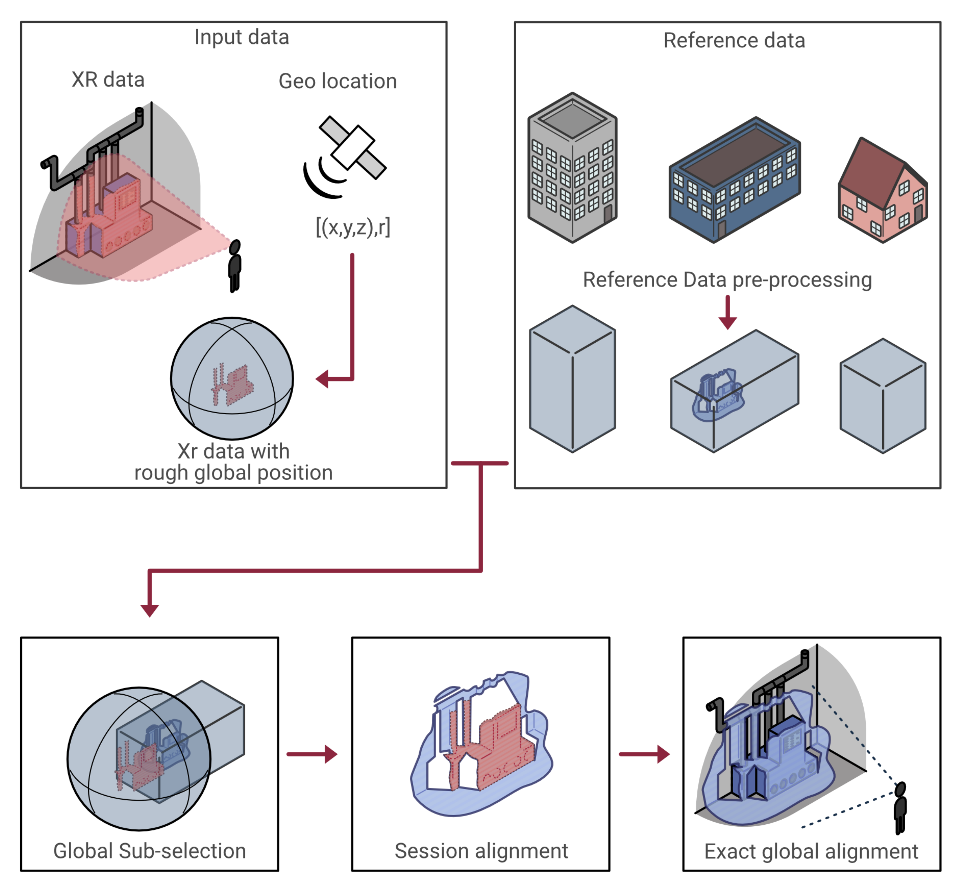
This section explains the overall structure of the method. Concretely, we discuss (1) the data preprocessing for the BIM, image, and geometry reference data and consecutive XR-data captures of a site; and (2) the global XR pose estimation per session based on visual and geometric features. It is important to notice that the continuous local pose estimation within a session by the Microsoft SLAM API (Scene understanding SDK), in combination with the Hololens 2, is left unaltered as it is proven to yield reliable and accurate results for small-scale scenes [20]. Instead, we pursue the localisation of the entire data acquisition session with respect to the facilities’ coordinate system in the cadre of interfacing with and updating the facilities’ digital twin (Figure 2).

3.1. Data Preprocessing

When handling a wide variety of datasets across different time periods, there must be a joint framework to link and jointly process the data. In this work, we will utilize the geospatial component of the remote sensing and BIM data to link the different datasets. When a surveillance is made, the captured data are generally stored with respect to a common reference point. This collection of data are referred to as a session. Sessions can contain images, meshes, point clouds, and even BIM models, all with their own relative transformation. All the data need to be geolocated, and since there are a number of different standards, it is important to always include which coordinate system is being used. The three most used in Belgium are: WSG, Lambert72, and Lambert2008. For this section, the reference and test data are handled separately. However, it is important to notice that each new session can be used as a reference for future test data and, thus, both data structures need to be standardized. To this end, semantic web technologies are leveraged to manage the spatial and temporal metadata of each reference dataset. Concretely, a set of light weight RDF graphs are constructed, which are updated with each new XR data capture. The geospatial data processing, metadata extraction, RDF graph conceptualization, and implementation of each dataset is discussed below.

3.1.1. Reference Data

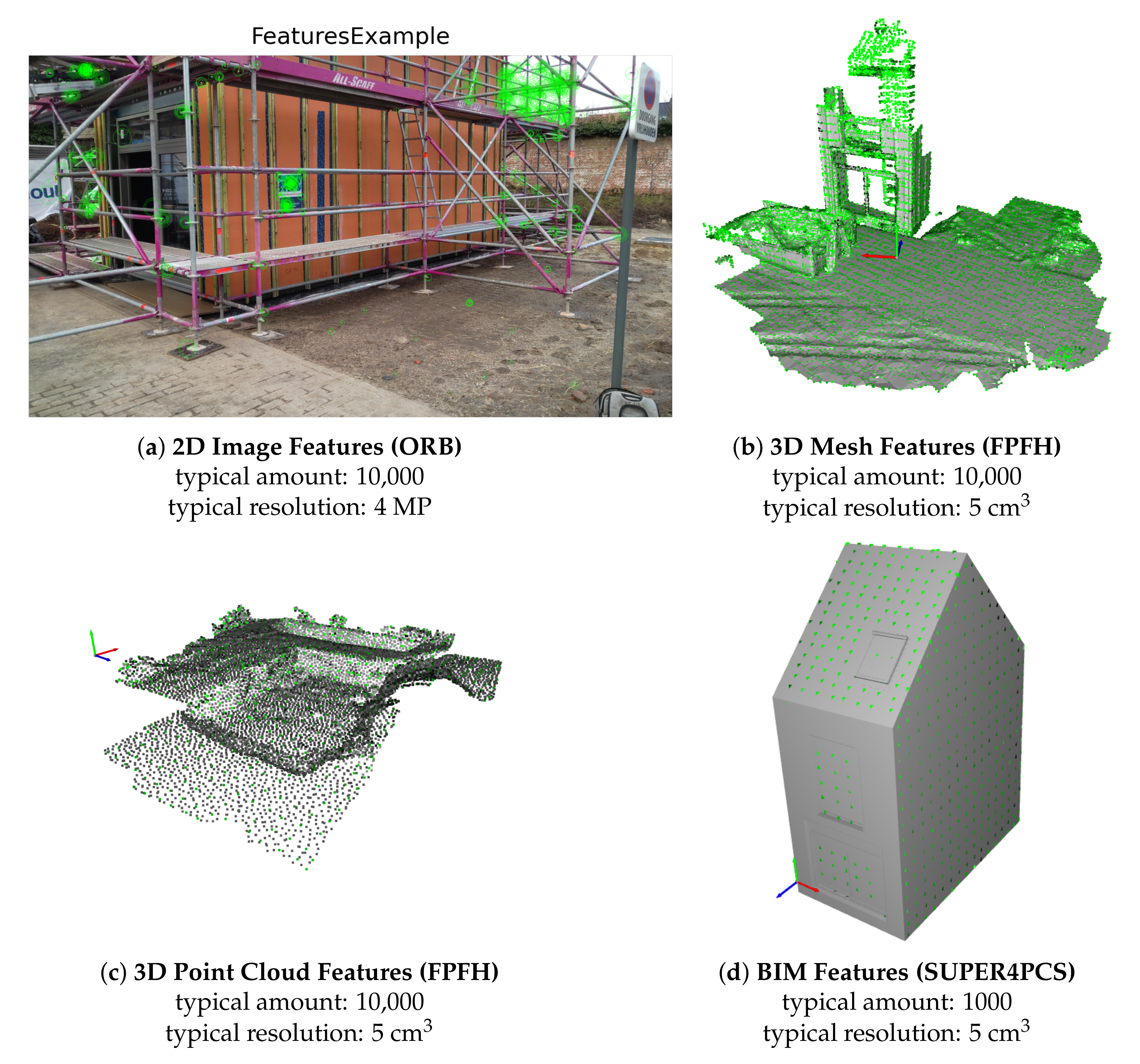
The following reference data are considered for the global pose estimation (Figure 3): the BIM digital twin in a preset coordinate system (preferably geolocated), Lidar data, localised image data, and XR data captured from previous sessions. These repositories are preprocessed and geolocated as follows.

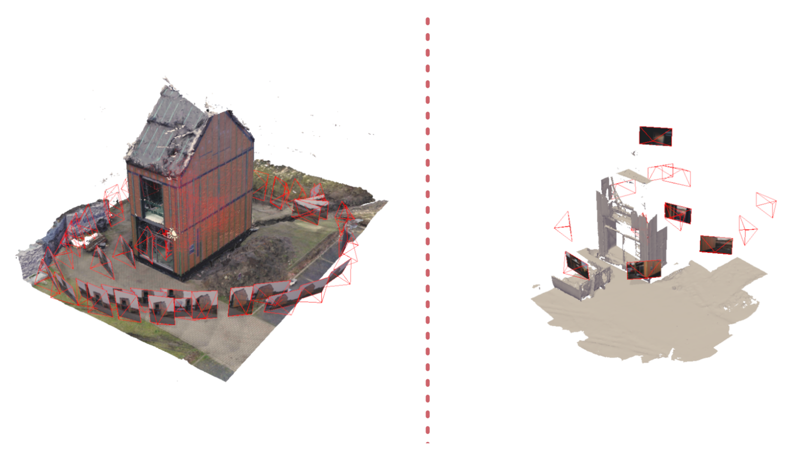
Imagery

The preexisting imagery of a facility is one of the most promising methods to align newly captured XR data (Figure 3a). There are iMMs and TLS images to consider, as well as panoramic imagery, images taken by smartphones, handheld cameras, and UAVs. The iMMs and TLS imagery are already localised during the Lidar registration processing. Other imagery is processed by structure-from-motion (SfM) software, such as MetaShape or RealityCapture, to estimate the camera’s interior and exterior orientation parameters, including the focal length, position, rotation, and so on. During this process, control points, either from Lidar, total station, or GNSS measurements, need to be manually added to the image collections to properly reference and scale the imagery. The result is a set of images accompanied with an RDF graph that contains the location and orientation of each image along with its camera parameters and timestamp. Additionally, the Oriented FAST and Rotated BRIEF (ORB) features extracted in the SfM pipeline are stored per image, so no additional preprocessing is needed in the pose estimation step.

Point Clouds

Facilities are increasingly scanned at key stages of their life-cycle, such as during construction, renovations, and so on. These captured data, either with static TLS or iMMs, generate a collection of Cartesian coordinates with optional colour and intensity values per setup or trajectory (Figure 3c). During the post-processing of these datasets, control points established with GNSS or total station are added to geolocate the resources. The geolocated points clouds in an E57 format are the starting point of our method. As our codebase operates in Open3D [27], each point cloud is converted to the PCD format. There are both ordered and unordered point cloud datasets to consider. For instance, .e57 point cloud files containing a collection of per setup captured structured point clouds are stored as separate PCD files. The e57xmldump tool [28] is used to first extract the E57 metadata information which is than parsed using the RDFlib API [29]. The resulting metadata is stored as triples in an RDF graph pcdGraph.tll which is serialized using the turtle syntax. During this operation, a heavily downsampled voxel octree and a set of Fast Point Feature Histograms (FPFH) geometric features is extracted from the Lidar data that will serve as reference for the pose estimation [30]. The octree and features are also stored in the RDF graph so they can be reused throughout consecutive pose estimations without the need to load the original point cloud data.

Polygonal Meshes

Polygonal meshes can both stem from remote sensing or from the Building Information Model (discussed below) (Figure 3b). The former is a direct product of XR device data captures, such as the Hololens 2 or the SfM pipelines as discussed above, that generate textured mesh geometry of the facility. Additionally, Lidar point clouds can be processed to polygonal mesh geometries using various meshing techniques, such as Poisson meshing variants [31]. The features that are extracted from the polygonal meshes are the same as those extracted from the point cloud data. To this end, point clouds are sampled on the mesh surfaces and subjected to the same feature extractors, as described above. Analogue to the point cloud processing, the features, bounding box, centroid, and so on are stored in an RDF graph.

Building Information Model

The geospatial representation of BIM elements can be either defined by BREP or polygonal mesh representations (Figure 3d). As such, they are compatible with the same code as for the polygonal mesh geometry processing. However, using the point cloud features on an abstract BIM model are likely to fail due to modeling abstractions and sparsity of the BIM. Therefore, plane-based descriptors are extracted from the BIM geometries and stored in an RDF graph bimGraph.ttl. Specifically, we extract Super4PCS features, as described in [32]. The descriptors are stored using their absolute coordinates, which also includes the translation and rotation of the BIM project with respect to the global coordinate system.

The main goal of the alignment is to position the XR device’s data in the world. For that, the reference data needs to be geolocated. There are a number of international standards for geolocating data, so each RDF resource is enriched with the coordinates system information that is being used. Each resource is also given an accuracy parameter which will play an important role in the pose estimation reliability. This accuracy metric is either directly obtained from the processing of the remote sensing data, i.e., the network error in Lidar networks or the mean error on the control points in a SfM pipeline. For the BIM geometries, a default 0.05 m accuracy is chosen as conform LOA20 [19], which is a safe option considering the common abstractions of BIM models.

3.1.2. XR Data Capture

This work focuses on cross platform compatibility, so we try to capture and link as much data as possible. Therefore, the codebase, which is developed in Unity3D, accepts common inputs from various XR devices. Specifically in this work, we build our framework against the Hololens 2 and Android smartphone inputs to showcase the multi-sensor inputs. Analogue to the reference data, the XR data are organised in periodic sessions. Each session contains a global reference point, a number of images and meshes. Since these data are captured (near) real time, the fidelity and file size is relatively small. This lowers the time to transfer files across devices and also the computation time. Note that it is not required to have both 2D and 3D data available in a session, as not all devices contain the necessary sensors to capture both. The pose estimation is specifically designed to deal with very limited data and provides different methods depending on the input.

Two-Dimensional Capture

Images are captured using the on-board device cameras. As previously mentioned, We rely on the XR SLAM capabilities to track the subsequent sensor poses within the session. As such, the relative location and orientation of the imagery is directly adopted into the RDF graph which is identical to the imageGraph proposed above. once a new image is captured by the device, it is send to a server that automatically extracts the relevant metadata and features and stores this information in the session’s RDF graph.

Three-Dimensional Capture

Some XR devices are equipped with special sensors that can capture depth, such as the ToF on the Hololens 2, or RGBD sensors of some Android devices. Using these data, the XR SLAM can create a real-time mesh of the environment. Specifically for the Mixed Reality API of the Hololens 2, the mesh is dynamically built from consecutive blocks of by default 8 m${}^3$. By default, the spatial resolution of the mesh is kept rather low to save computational resources, but this can be changed for a more detailed mapping. Because the generated mesh is spatially sub-sampled, the distance to the environment is largely irrelevant as long as the structure remains within range of the sensor. Once a number of cells is captured, the mesh is sent to the server where it can commence the 3D pose estimation process. To this end, an RDF Graph similar to the meshGraph defined above is generated from the raw mesh and serialized in a .ttl file.

3.1.3. RDF Schema

There is a clear need for standardisation, due to the fact that a lot of the reference data will come from diverse sources and different periods throughout the building’s life-cycle. Properties such as an id, position, and rotation already have strict schemes built out, so it is imperative that we use the same standards. Currently, we implement RDF, RDFS for the general concepts. GEO is used overall to represent the geospatial information of the resources, while EXIF is specifically used early on to extract the metadata from the images. We rely on OMG for the geometry definitions and the pathing of each session. For the sensory metadata, including the position, centroid, bounding box, number of points, vertices, faces, and so on, we use the OpenLabel which is extensively used for mobile mapping and navigation data. Finally, the Image, Mesh, and Point Cloud classes are designed on top of our V4Design ontology and have a series of relationships that govern exchange of information between the classes [33]. A feature relation is also defined to store the resources’ 2D and 3D features along with the description of the feature type (ORB, SIFT, etc.). The Arpenteur [34] ontology is also used that already defines a number of relationships for SfM processes and fits well with this framework.

3.2. Pose Estimation

In this section, the pose estimation of the session is presented. The alignment is divided into two consecutive steps. First, an approximate global pose request is processed by the XR operator’s android device to narrow the search area for the pose estimation. In a second step, an exact pose estimation is calculated using the XR captured data and the above described reference datasets. In the following sections, the global pose estimation and the subsequent 2D and 3D pose estimations are discussed in detail.

$s\in S$ is a session that contains some point clouds $P_s\in {\mathit{P}}_{\mathit{s}}$ (either from meshes, depth imagery or structured point clouds) and images $i_s\in I_s$. From the preprocessing, every $P_s$ has an RDF graph $G_{P_s}$ that contains its metadata, a set of distinct 3D points $X_s$ and 3D feature vectors $F_{3D}$. Analogue, every $i_s$ is stored in an RDF graph $G_I$ that contains the metadata, a set of distinct 2D pixels $x_s\in {\mathit{x}}_{\mathit{s}}$ and 2D feature vectors $F_{2D}$.

R are all the reference datasets that each contain some point clouds $P_r\in {\mathit{P}}_{\mathit{r}}$ (either from meshes, depth imagery, structured point clouds or the Building Information Model) and images $i_r\in I_r$. From the preprocessing, all $P_r$ are stored in an RDF pcdGraph $G_P$ that contains the metadata, a set of distinct 3D points $X_r$ and 3D feature vectors $F_{3D}$ of each resource. Analogue, the $i_r$ are stored in and RDF imageGraph $G_I$ that contains the metadata, a set of distinct 2D pixels $x_r\in {\mathit{x}}_{\mathit{r}}$ and 2D feature vectors $F_{2D}$ of the images.

3.2.1. Global Alignment and Reference Data Selection

As already mentioned, the bulk of the calculation will be performed on a server in order to ensure a smooth operation of the device and give access to all the reference data. The server is build in python, using the Flask framework. It is critical that the server has access to the reference data and has enough computing power too compute the tasks. The data captured on the XR device is organised in a session and send as a whole to the server, where it can be prepared for the pose estimation.

The first step of the alignment process is the sub-selection of reference data. Due to the large amount of reference data, it is not feasible to use every session in the pose estimation. This selection is performed by using the global pose retrieved from the XR device or another device in the general vicinity based on the HTML Geolocation API [35]. A positioning query is formulated on OpenStreetMap data using the Overpass API which generates a HTTP GET request, and receives a response in XML format. In the GNSS thread, a query is executed at the system start up, using the initial user position and a threshold radius. After this, a new query is executed when the user has moved significantly from the starting location given a distance threshold with respect to the last executed query. Since the device can be indoors or lack a GPS, the retrieved geolocation is not necessarily very accurate, with a error radius of circa 20 m. However, this is sufficient to narrow down the available reference data to reduce the computational effort of the precise localization algorithm.

The result of this query is the initial session pose $[p_s\pm {\sigma }_g]$ with the positioning accuracy as determined by the Wi-Fi, radio, and GNSS availability near the receiver. Given the pose, the relevant subsets of ${\mathit{P}}_{\mathit{r}}$ and $I_r$ are extracted. To this end, the Euclidean distance is evaluated between the focal point of each session image $i_s\left(c\right)$ and the focal point of each reference image $i_r\left(c\right)$. Analogue, when a session point cloud $P_s$ falls within the boundaries of a reference point cloud $P_r$ considering ${\sigma }_g$, the cloud is withheld as a valid reference (Equation (1)) (Figure 4).

$$\begin{array}{cc}\hfill & {\mathit{P}}_{\mathit{r}}^{\prime }=\left\{P_r\in {\mathit{P}}_{\mathit{r}}|P_r\cap \left[P_{s,min}-{\sigma }_g;P_{s,max}+{\sigma }_g\right]\right\}\hfill \\ \hfill & I_r^{\prime }=\left\{i_r\in I_r|i_s\in I_s:\parallel i_r\left(c\right)-i_s\left(c\right)\parallel \le t_d+{\sigma }_g\right\}\hfill \end{array}$$

(1)

where threshold $t_d$ serves as the distance threshold to limit the number of selected images. From the subsets ${\mathit{P}}_{\mathit{r}}^{\prime }$ and $I_r^{\prime }$, the relevant graphs $G_P$ and $G_I$ are retrieved along with the 2D and 3D features. Overall, this selection step significantly lowers the computational complexity of the matching if a descent pose estimation accuracy is achieved. Moreover, the selection itself is also extremely efficient as the input variables are directly taken from the metadata graphs instead of having to transfer and evaluate the actual imagery and point cloud data.

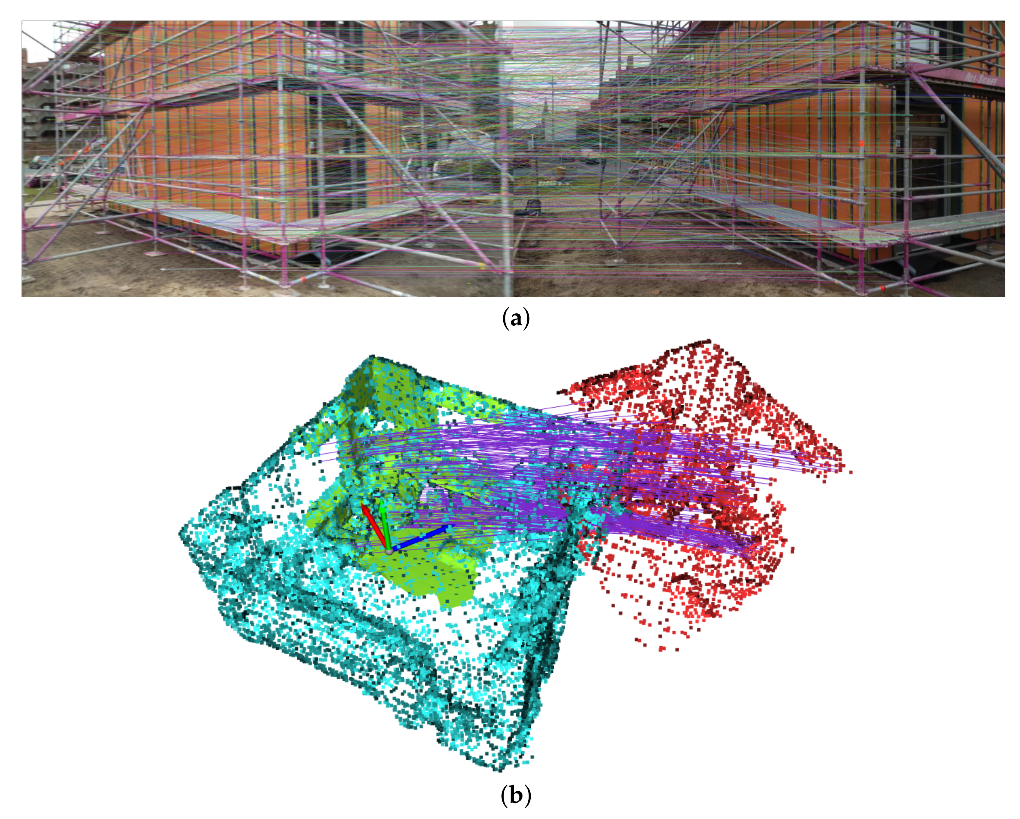
3.2.2. Three-Dimensional Pose Estimation

Point Clouds and Meshes

Given the 3D FPFH features of every reference point cloud and the session point cloud, a rigid body transformation is computed. To this end, a Fast global registration is applied as proposed by Zhou et al. [36]. We specifically do not use ICP variants as it would require the transfer of all reference clouds to the server. Additionally, the method of Zhou et al. foregoes computationally demanding RANSAC variants for the correspondence matching and instead propose a correspondence estimation function. Concretely, the distances between correspondences $X_s^{\prime }\in X_s$ and $X_r^{\prime }\in X_r$ are minimized while simultaneously the correspondence outliers are neglected by the correspondence estimation function $\rho$ (Equation (2)) (Figure 5).

$$\begin{array}{cc}\hfill & \underset{{\mathit{T}}_{P_s}}{argmin}\sum _{X_r^{\prime },X_s^{\prime }}\rho \left(\parallel X_r^{\prime }-{\mathit{T}}_{P_s}{X}_s^{\prime }\parallel \right)\hfill \end{array}$$

(2)

where the target rigid body transformation ${\mathit{T}}_{P_s}$ between a reference cloud and the session cloud is found by minimizing the distance between correspondences in $X_s$ and $X_r$. Both for the feature descriptors and the rigid body transformation estimation, the Open3D framework is implemented based on the work of Zhou et al. [36]. As previously mentioned, only the feature graphs are transferred to the server and, thus, only the transformation estimation is calculated in runtime which frees up computational resources. The resulting pose, as well as the RMSE, the number of inlier correspondences, and the bounding box of the inlier correspondences are stored with a relation to the reference point cloud. These metrics will be later used in the final pose estimation.

BIM Alignment

The same logic is applied to the BIM model. Given the sampled meshes, SUPER4PCS is used as described by Mellado et al. [32]. The approach relies on approximately congruent 4-point sets from a 3D point cloud that can be related by rigid body tranformations. A key innovation over the established 4-Points Congruent Sets (4PCS) algorithms is the computational dimensionality reduction from $O(n^2+k)$ to $O(n+k)$, where k is the number of reported sets, of the pairing problem and a smart indexing scheme to filter all the redundant pairs in the second stage. As the verification steps remains the same as the above procedure (using k sets instead of X), Equation (2) is also valid for the BIM transformation assessment. Additionally, the same metrics are stored in the RDF graph including the RMSE, the number of inlier correspondences and the bounding box of the inlier correspondences.

3.2.3. Two-Dimensional Pose Estimation

Given the 2D ORB features of every reference and session image, a transformation matrices can be computed for every image in the session using state-of-the-art SfM methods. The camera pose of a session image ${\mathit{T}}_{i_s}$ in relation to the global coordinate system is given by the rotation matrix ${\mathit{R}}_{i_s}$ and the camera position of image ${\mathit{t}}_{i_s}$. The relation between the matched 2D pixels $x\in \mathit{x}$ of an image $i_s$ and their 3D projections $X\in \mathit{X}$ can then be defined as follows (Equation (2)).

$$\begin{array}{cc}\hfill & x=\pi ({\mathit{T}}_{i_s},X)=\mathit{K}\left[\begin{array}{cc}{\mathit{R}}_{i_s}^T& -{\mathit{R}}_{i_s}^T{\mathit{t}}_{i_s}\\ 0& 1\end{array}\right]X\hfill \end{array}$$

(3)

where both X and x are represented by their homogeneous coordinates. $\mathit{K}$ is the camera intrinsic parameters matrix. To estimate the camera poses of all $i_s\in I_s$, the following energy function can be minimized through bundle adjustment [38] (Equation (4)).

$$\begin{array}{cc}\hfill & \underset{{\mathit{T}}_{i_1}...{\mathit{T}}_{i_s}}{argmin}\sum _{I_s,I_r}\sum _{\mathit{X}}\rho \left(\parallel \pi ({\mathit{T}}_{{\mathit{i}}_{\mathit{s}}},\mathit{X}){-\mathit{x}\parallel }^2\right)\hfill \end{array}$$

(4)

where $\mathit{X}$ and $\mathit{x}$ are the combined matches for the session s. A similar loss function $\rho$ as in Equation (2) is defined to down-weigh potential outliers. To minimize Equation (4), a number of methods can be employed. In this work, we use the OpenCV Levenberg–Marquardt implementation [39]. It is important to notice that the resulting ${\mathit{T}}_{i_s}$ is not yet scaled. To solve the scale, we identify three cases to estimate the scale that will occur in XR data capture.

Two Overlapping References

If a session image $i_s$ can be matched with at least two overlapping reference images $I_r^{\prime }=\{i_{r_1},i_{r_2}\}$, the global pose of the session image ${\mathit{T}}_{i_{s,g}}$ is retrieved by solving Equation (1) using at least 6 3D–2D point correspondences. These correspondences $\mathit{X}$ are already determined in the global coordinate system due to the global pose of $i_{r_1}$ and $i_{r_2}$ (Figure 6a).

Two Separate References

In the case that two non-overlapping reference images $I_s=\{i_{r_1},i_{r_2}\}$ can be matched to the session image $i_s$, the global pose of the session image ${\mathit{T}}_{i_{s,g}}$ is retrieved by evaluating the relative transformations between $i_s$ and $i_{r_1}$ and $i_{r_2}$, respectively (Figure 6b). To this end, the average pose is taken considering the accuracy of the absolute poses ${\mathit{T}}_{i_{r_1,g}}$ and ${\mathit{T}}_{i_{r_2,g}}$.

One Reference Image with Geometry

In the case that only a single reference image $i_r$ can be matched to the session image $i_s$, but their point cloud present in the session or the reference, the global pose of the session image ${\mathit{T}}_{i_{s,g}}$ is retrieved by ray tracing $\mathit{x}$ (Figure 6c). To this end, a set of rays $l(c,x)\in L$ is constructed from the focal point $i_s\left(c\right)$ or $i_r\left(c\right)$ through $\mathit{x}$ depending on whether the geometry is part of the session or the reference. The intersection between the geometry P and L than yields the 3D coordinates of the 3D correspondences $\mathit{X}$ (Equation (5)).

$$\begin{array}{cc}\hfill & \mathit{X}=\left\{p\in P\left|l\right(c,x)\in L:p=l(c,x)\cap P\right\}\hfill \end{array}$$

(5)

3.2.4. Final Pose Estimation

Given the above pose candidates per session and per resource, the final transform ${\mathit{T}}_s$ is computed based on a weighted pose vote over all point cloud and image transformations $\mathit{T}=\{{\mathit{T}}_{\mathit{P}},{\mathit{T}}_I\}$ in a session (Equation (6)).

$$\begin{array}{cc}\hfill & {\mathit{T}}_P=\frac{1}{n}\sum _{\mathit{T}}\omega \left({\mathit{T}}_{\mathit{P}},{\mathit{T}}_I\right)\hfill \end{array}$$

(6)

where the weight $\omega$ of each resource is computed for image transformations based on the reprojection error, the number of matches, inlier percentage, and bounding box of the inliers. For point cloud transformations, $\omega$ is established based on RMSE on the matches, the number of matches, the bounding box of the matches. For these transformations, the theoretical sensor accuracy is also taken into account. Every parameter is normalized to ensure larger numbers do not disproportionately affect the final weight. Every type of registration also contributes to the weight as follows based on empirical and theoretical evidence: Super4PCS alignment (1), SfM with two overlapping references (0.8), FPFH features with a measured point cloud(0.8), two separate reference images (0.5) and one reference image but with geometry (0.4).

4. Test Data

Three periodic test cases were captured and processed of both operational facilities and buildings under construction (

Table 1. Overview of the provided reference data of test cases 1 and 2.

		# Sessions	# Images	# 3D Objects	# Points	# Downsampled Points	Typical Image Resolution
1 Campus	BIM	3	/	186	3,980	82,050	/
	VLX	3	241	3	162,108,105	2,481,633	2048 × 1042
	Hololens	6	35	483	1,089,574	16,679	3904 × 2196
		# sessions	# images	# 3D objects	# points	# downsampled points	Typical image resolution
2 Living Lab	BIM	1	/	368	41,825	41,351	/
	P30	1	274	2	7,638,931	565,938	640 × 640
	Photogrammetry	3	642	3	1,013,736	75,103	4240 × 2832
	Hololens	5	30	15	439,816	32,584	3904 × 2196

). In total, 45 sessions were documented using static TLS with a Leica P30 and Leica BLK, the indoor mobile mapping system NavVis VLX, a CANON EOS 5D MARK II, the Microsoft Hololens 2, and conventional smartphones. The raw images and point cloud data were manually processed to serve as a baseline for the analysis of the two-step alignment. The camera poses of the images were retrieved by using the Reality Capture SfM pipeline and the optimized poses of the iMMs and TLS sensors. The Android smartphone and Hololens 2 datasets were then manually registered to these inputs and used as the baseline for the comparison. Specifically for the Hololens 2, the 3D meshes were captured with an average density of 0.08 m${}^3$. The data were captured with a custom-made application created with the Unity3D game engine and send to the local web server. Some sessions were taken with an android smartphone using the same application, but due to hardware limitations, these sessions only contain images. The rough global pose was captured using regular android phones and the data were sent to the same server to store for the fine pose estimation.

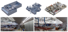
The first test case is the soil technology lab on our Campus in Ghent (Table 1 row 1). It is a laboratory space that resembles an industrial site and houses working desks, machinery, bulk materials, and so on. Between the periodic data captures taken in several months, the lab was operational and, thus, all movable objects were displaced in the documented period. As such, this test cases focuses on the ability of the fine-alignment to register multi-temporal inputs of an operational environment. With a size of 10 m × 30 m, it is also circa the size the Hololens 2 can capture conform LOA20 [2$\sigma \le$ 0.05 m] without the inclusion of the control points. For this test case, a basic BIM is available of the structure.

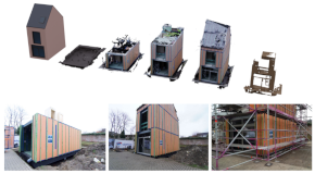
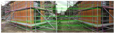
The second test case is the construction of a prefab living lab on the Technology Campus (Table 1 row 2). This project was periodically captured with the different sensors starting from the early stake-out all the way to the MEP installations. The structure itself is a three-storey building that resembles an office/housing space and was constructed from prefab structure elements. As such, this test case focuses on the robustness of the algorithm to match the data of different sensors in an outdoor construction site environment that is drastically changing in both texture and geometry. For this test case, a detailed as-designed BIM is available of the structure, architectural finishes, and MEP installations. The full construction was documented using both a Sony a6400 camera, used for photogrammetric reconstruction, and the Hololens 2, for subsections of the building.

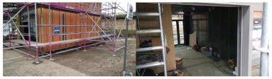
The last test case is a renovation of a house in Brugge (

Table 2. Overview of the provided reference data of test case 3.

		# Sessions	# Images	# 3D Objects	# Points	# Downsampled Points	Typical Image Resolution
3 House	BIM	1	/	594	24,783	84,031	/
	P30	1	/	20	264,525,819	19,597,665	/
	Photogrammetry	1	430	0	/	/	5616 × 3744
	Hololens	20	91	18	378,075	28,010	3904 × 2196

). The refurbishment was periodically captured both by smartphones and the Hololens 2 and has Leica BLK data as a baseline. The structure consists of a four-storey building including a full-storey basement and attic. This test case focuses on the robustness of the algorithm to match data of different sensors on an indoor construction site environment that is drastically changing in texture and where there is a lot of clutter and temporary storage of materials. For this test case, a detailed as-built BIM is available of the structure and architectural finishes.

5. Experiments

In the following section, the different pose estimation methods and the final parameters to determine the best overall pose are evaluated. The accuracy is based on the distance error (m) and angle error (deg), which indicates the distance and angle difference between the estimated transformation and the correct pose, respectively. Additionally, as stated before in Section 3.2, the pose is determined based on a weighted pose vote of five methods (two Lidar and three image-based). Each method has distinct advantages and disadvantages in specific use cases, and so there are a number of parameters to evaluate which method works best in which case. Each method is evaluated using the same parameters based on the best fit parameters that were empirically determined over all measurements. The global distance threshold $t_d=10$ m was set based on a relevant ground sampling distance for smartphones (avg. 12 MP), mirrorless cameras (avg. 24 MP), the Hololens 2 (12 MP) and the TLS and iMMs image (5 MP) and Lidar resolution (avg. 10 MP). The feature correspondence functions $\rho$ for the image and Lidar matches was set, respectively, to 50 pixels and 1.5 times the voxel size (0.05 m) to mitigate the noise on the changed environments. The weights for each method $\omega$ were distributed based on the number of successful test cases of each method: FPFH features with a measured point cloud (0.8), SfM with two overlapping references (0.8), one reference image but with geometry (0.4), two separate reference images (0.5), and SUPER4PCS alignment (1).

The order in which the experiments are presented is the following. First, the performance of each method is presented based on good and bad performances of the methods on test case 2 as it is the most varied dataset with significant matching challenges. The quality and parameters of each method are discussed in detail to conclude where each method will fail and succeed (Figure 7). Second, the general pose voting results are discussed over all three test cases given the confidence levels of each method. Based on the test results, it is determined in which type of scenarios XR-devices will be able to align with preexisting datasets and which sensor data are preferred to achieve the highest quality alignment in construction site environments.

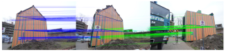
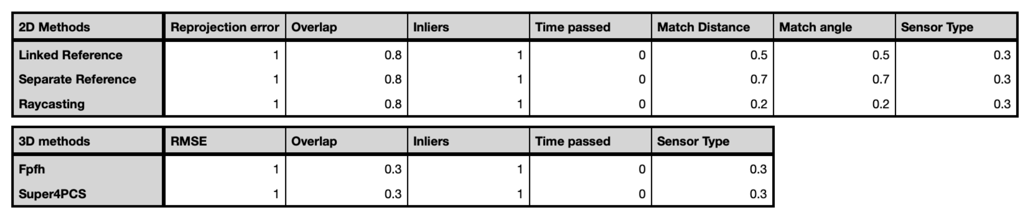
5.1. Two-Dimensional Alignment

The 2D alignment methods are based on the OpenCV ORB feature matching. The accuracy of the alignment is, therefore, reliant on the quality of each match. Since only one or two matches are required for the alignment, only the best matches are retained for the next step. The quality of each match is directly evaluated by comparing the reprojection error, inlier percentage and overlap of the proposed transformation between the two images.

Table 3. Examples of a correct and incorrect image match.

Sensor	reprojection	Overlap	Inliers	Time	Match	Match
	error (pix)	(%)	(%)	Passed (days)	Distance (m)	Angle (deg)
Hololens	30.4	60.0	53.7	3	3.41	11.28
Sensor	reprojection	Overlap	Inliers	Time	Match	Match
	error (pix)	(%)	(%)	Passed (days)	Distance (m)	Angle (deg)
Hololens	38.6	5.7	5.0	3	8.01	71.80

shows clear examples of a correct and incorrect match between two session images. The incorrect match easily stands out due to its 5% inliers and limited overlap. These parameters are, thus, excellently suited to determine the matching quality with varying combinations of reference and test data.

5.1.1. Two Overlapping References

The first method is used when there are sufficient overlapping images between the reference and test session. The results can be found in

Table 4. Two-dimensional matching estimations based on 2 linked reference images.

Sensor	Distance	rotation	Reprojection	Overlap	Inliers	Time	Match	Match
	Error (m)	Error(deg)	Error (pix)	(%)	(%)	Passed (days)	Distance (m)	Angle (deg)
Sony APSC	0.10	0.46	28.10	49.5	50.0	1	2.09	7.85
Sensor	Distance	rotation	Reprojection	Overlap	Inliers	Time	Match	Match
	Error (m)	Error(deg)	Error (pix)	(%)	(%)	Passed (days)	Distance (m)	Angle (deg)
Hololens	0.39	3.35	28.77	31.7	34.3	1	4.50	12.6

where it is clear that this method works best for reference sessions with a large amount of images with high overlap. This is found mostly with photogrammetry reconstructions, since this is essentially the same method being used.

Since the session scaling comes from the relative distance between the two reference images, larger distances generally yield more exact scale estimations. However, as the relative distance increases, the overlap of the image generally also decreases, resulting in a worse match. For instance, the matching of the top image in Table 4 yields a distance error of 0.1 m and is based on two highly reliable image matches on two images taken 2 m apart on consecutive days. The bottom image has matched to two images taken 4.5 m apart which would theoretically increase the accuracy. However, the poor image matching (only 34% inliers and 20% overlap) actually leads to an inferior pose estimation. As such, good image matches are prioritized over larger baselines for the final pose estimation.

As expected, this method under-performs in sparse image datasets, where reference session matches are both rare and of poor quality. This is the case when significant texture changes have taken place on the construction site or facility, e.g., plastering or painting of the interior. Additionally, in case a good match is found between a test image and a reference image, but the reference image does not have a good other match, the method will under-perform. It is, therefore, essential that the bad reference match has enough weight in the pose estimation to ensure it does not obtain a high confidence, e.g., by only retaining the parameters of the worst match of the pair.

5.1.2. Two Separate References

The second method is used when two separate matches are found between session and reference images. Both matches are then cross referenced to calculate the final pose of the image. The results can be found in

Table 5. Two-dimensional matching estimations based on 2 separate reference images.

Sensor	Distance	rotation	Reprojection	Overlap	Inliers	Time	Match	Match
	Error (m)	Error(deg)	Error (pix)	(%)	(%)	Passed (days)	Distance (m)	Angle (deg)
Sony APSC	0.15	0.92	27.66	57.6	21.4	1	12.81	64.38
Sensor	Distance	rotation	Reprojection	Overlap	Inliers	Time	Match	Match
	Error (m)	Error(deg)	Error (pix)	(%)	(%)	Passed (days)	Distance (m)	Angle (deg)
Sony APSC	2.20	0.69	33.06	17.2	28.9	1	2.09	7.85

where it is clear this method works best for reference sessions where sporadic images are taken in a large area of the site. This case happens mostly with mobile mapping systems, such as XR datasets or the VLX datasets, that only store imagery at key locations that do not necessarily have overlap between them.

For the cross referencing of the pose estimation, an important factor is the relative angle between the two estimated positions to ensure a high confidence. When the direction of the matches are more perpendicular than parallel, small deviations in the directions become less pronounced and, thus, increase the accuracy of the resulting intersection. Similarly, near parallel matches have a larger depth error. The relative distance also negatively impacts the result as larger distances increase the deviation of small directional errors. This effect is demonstrated in Table 5 where the top match yields a descent pose estimation despite the average matching statistics due to the high rotational angle between both reference images (64.38${}^{\circ }$). Instead, the better matching bottom image only has an angle of 7.85${}^{\circ }$ between both references, causing a significant distance error.

This method will also under-perform when the reference images are positioned too close to the session image as this drastically amplifies the rotational error. As such, the best match for this method is based on the matching angle of both references and the intermediate Euclidean distance between them.

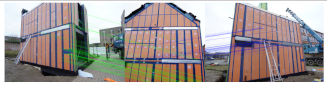
5.1.3. One Reference Image and 3D Data

The third method is used if only one good match can be found in the reference images and there are 3D data available, either in the test or reference session. In this case, the correspondences of the matching images are raytraced on the present geometries to determine the scale. The results can be found in

Table 6. Two-dimensional matching estimations based on 1 reference image and a Mesh.

Sensor	Distance	Rotation	Reprojection	Overlap	Inliers	Time	Match	Match
	Error (m)	Error(deg)	Error (pix)	(%)	(%)	Passed (days)	Distance (m)	Angle (deg)
Sony APSC	0.02	0.01	23.8	36.8	52.2	2	2.22	15.22
Sensor	Distance	rotation	Reprojection	Overlap	Inliers	Time	Match	Match
	Error (m)	Error(deg)	Error (pix)	(%)	(%)	Passed (days)	Distance (m)	Angle (deg)
Sony APSC	1.88	3.45	36.2	31.7	10.9	4	4.54	18.89

. Since this method requires 3D data to be available, it rules out some of the more basic datasets that lack 3D data. However, when such a dataset is available and if the 3D data have enough coverage of the area from the camera’s point of view, this method shows promising results. This methods preforms well on all test cases that contain 3D datasets and the minimal required images can be very low since only one images needs to be matched.

There are three important factors that influence the pose estimation: (1) A sufficient distribution of depth information of the raycast image matches is necessary to establish the correct scale of the pose. (2) Any artefacts in the 3D data such as ghosting or noise on windows can obstruct the raycasting, resulting in an erroneous scale. RANSAC filtering is therefore mandatory for retrieving the correct distances. (3) The accuracy of the 3D data itself directly effects the accuracy of the pose estimation. For instance, the Hololens 2 has a limited depth accuracy compared to high-end TLS or iMMs which translates to a reduced pose accuracy. It should also be noted that since point clouds lack a surface definition, the resulting voxel raytracing algorithm [40] will result in less precise results compared to meshes, which do have a surface definition. Overall, the top image shows a high distance (0.02 m) and rotation accuracy (0.01°) can be obtained when matching with combined high-end TLS and Hololens 2 data.

This method fails when the available 3D object either has to little coverage from the camera’s point of view, since there will be insufficient data points to compare, or the dataset contains to much noise, resulting in several scale factors that cannot be reliable filtered by RANSAC. This is the case with the bottom image in Table 6 where the image matches lead to an erroneous raycasting in occluded areas.

5.2. Three-Dimensional Alignment

The 3D matching methods are based on two different feature matching frameworks. Open3d uses FPFH features while Super4PCS is a more robust matching algorithm that requires less matches. In contract to the image matches, a single alignment between a reference and a test session dataset is sufficient to position a session. The quality of each match is directly evaluated by comparing the percentage of feature inliers, a measure for the distribution of the overlap and the RMSE of the matches.

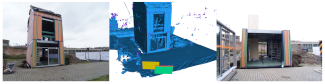
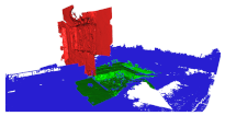
5.2.1. FPFH Feature Matching

FPFH feature matching is specifically designed to estimate the transformation between two observed point clouds as it determines features of all points in the cloud. This is why all 3D data are both converted to point clouds and subsampled to improve the speed of the algorithm. As seen in

Table 7. Three-dimensional matching estimations based on FPFH feature matching.

Sensor	Distance	Rotation	RMSE	Overlap	Inliers	Time
	Error (m)	Error(deg)	Error (m)	(%)	(%)	Passed (days)
P30	0.04	0.02	0.03	95.0	100.0	3
Sensor	Distance	Rotation	RMSE	Overlap	Inliers	Time
	Error (m)	Error(deg)	Error (m)	(%)	(%)	Passed (days)
BIM	3.56	90.45	0.70	20.0	15.0	31

, this method works best for point clouds with limited geometric changes over time, e.g., after the structure phase. As long as a large portion of the point clouds remains the same, the algorithm is able to correctly determine the correct pose. For instance, the top image in Table 7 shows a good match between the finished ground works and the placement of the foundations since the majority of the excavation pit was unaltered. However, after the structure was completed, the bottom image in Table 7 shows an incorrect match even though the surroundings of the structure are still the same.

An important factor for the success of FPFH or other point-based features is the presence of geometric detailing in the scene. The excavation of a construction site offers a large number of unique points of which the gradients results in a distinct and reliable feature. The method will, thus, underperform in scenes where only flat non-distinct geometries are found. Additionally, small amounts of overlap or ill-distributed feature matches will result in incorrect alignments as evidenced in the bottom figure of Table 7.

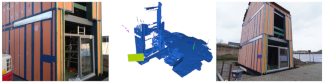
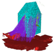
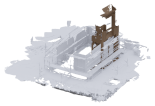
5.2.2. SUPER4PCS Feature Matching

When certain 3D datasets lack geometric detailing, such as a BIM model, a more robust method is required to match the different datasets. SUPER4PCS is specifically designed to overcome this lack of detailing by evaluating the geometric ratios between feature points. As seen in

Table 8. Three-dimensional matching estimations based on Super 4 PCS matching.

Sensor	Distance	Rotation	LCP score	Overlap	Inliers	Time
	Error (m)	Error(deg)	(%)	(%)	(%)	Passed (days)
BIM	0.09	3.35	70.4	15.0	60.0	31
Sensor	Distance	Rotation	LCP score	Overlap	Inliers	Time
	Error (m)	Error(deg)	(%)	(%)	(%)	Passed (days)
Hololens	4.56	90.50	3.2	30.0	3.0	5

, this method works best for database matching, such as with the as-designed BIM model and only requires a small subset of well documented planar objects to retrieve the correct alignment. For instance, the top figure in Table 8 shows only a 0.09 m error between a Hololens 2 dataset and the BIM model despite that only of small portion of the front of the structure (15% overlap) was captured in an area filled with noise and ghosting from the main window on the ground floor.

In contrast to the FPFH matching, the lack of geometric primitives in the scene can hinder the alignment. For instance, the bottom figure in Table 8 shows an incorrect match between two Hololens 2 data captures 5 days apart with mostly geometric details and not so much of the structure being documented. As such, FPFH and SUPER4PCS are complementary techniques that, if used in parallel, will lead to a more robust pose estimation framework.

5.3. Weighted Pose Estimation

Each method returns an estimated pose with various parameters.

Table 9. Positional and rotational results and the confidence of each method across the sessions of each test case.

Method		Linked Ref	Separate Ref	Raycasting	FPFH	SUPER4PCS	Combined
Estimated time		1–10 images/s	1–10 images/s	0.2–2 images/s	5 s–2 min/pcd	20 s–5 min/pcd	20 s–15 min/session
Method weight		0.8	0.5	0.4	0.8	1
Case 1	Positional RMSE (m)	0.145	0.189	0.021	0.159	0.061	0.065
	$\Delta$ Pos x (m)	−0.095	0.062	−0.018	−0.070	0.010	−0.017
	$\Delta$ Pos y (m)	−0.002	−0.165	0.008	0.030	−0.060	−0.038
	$\Delta$ Pos z (m)	0.110	0.068	0.008	0.140	0.008	0.050
	Rotational RMSE (deg)	0.960	0.636	0.189	1.507	0.463	0.538
	$\Delta$ Rot x (deg)	0.600	0.450	0.080	0.300	0.040	0.207
	$\Delta$ Rot y (deg)	0.600	0.450	0.170	0.470	0.300	0.369
	$\Delta$ Rot z (m)	−0.450	−0.003	0.020	1.400	0.350	0.332
	Confidence (%)	30.100	29.900	52.200	33.900	77.300	46.951
Case 2	Positional RMSE (m)	0.183	0.133	0.277	0.059	0.071	0.035
	$\Delta$ Pos x (m)	−0.143	0.043	0.037	0.050	0.003	0.007
	$\Delta$ Pos y (m)	−0.084	−0.095	0.266	0.004	0.070	0.032
	$\Delta$ Pos z (m)	0.078	−0.082	0.069	0.032	−0.010	0.013
	Rotational RMSE (deg)	0.993	1.207	0.018	0.156	0.028	0.074
	$\Delta$ Rot x (deg)	−0.887	0.706	0.006	0.020	0.001	−0.055
	$\Delta$ Rot y (deg)	0.229	−0.960	0.017	−0.120	0.020	−0.049
	$\Delta$ Rot z (deg)	−0.384	0.190	−0.003	0.097	0.020	0.010
	Confidence (%)	25.100	17.000	19.200	80.000	90.000	54.360
Case 3	Positional RMSE (m)	0.149	0.103	0.106	0.067	0.078	0.074
	$\Delta$ Pos x (m)	0.099	0.098	0.050	−0.005	0.030	0.031
	$\Delta$ Pos y (m)	0.099	0.026	0.078	0.030	0.004	0.028
	$\Delta$ Pos z (m)	0.053	0.013	0.052	0.060	0.072	0.061
	Rotational RMSE (deg)	0.852	1.073	0.713	0.966	0.171	0.399
	$\Delta$ Rot x (deg)	0.340	−0.890	0.670	0.890	0.030	0.322
	$\Delta$ Rot y (deg)	0.179	0.600	−0.050	0.430	0.100	0.234
	$\Delta$ Rot z (deg)	−0.760	−0.005	0.240	−0.120	0.135	−0.033
	Confidence (%)	20.200	21.900	31.400	67.000	75.000	48.077
Average	Positional RMSE (m)	0.159	0.141	0.135	0.095	0.070	0.058
	Rotational RMSE (deg)	0.935	0.972	0.307	0.886	0.221	0.337
	Confidence (%)	25.133	22.933	34.267	60.300	80.767	49.796

shows the accuracy of the pose estimation of each method in relation to its calculated confidence based on the chosen parameter modifiers. The exact values of these modifiers were determined based on empirical evidence from the test data and are outlined in Figure 7. The resulting confidence is the combination of the best estimations per evaluated sessions. These confidence parameters are each multiplied by its empirically determined method weight. The combined result determines the influence of each method on the final pose estimation. The accuracy is similarly computed by determining the weighted average for each axis based on the combined confidence and method weight parameters. As such, the outcome of the method is both a pose and a measure of agreement in confidence, position, and rotational accuracy.

The average positioning accuracy across the different test cases is 0.06 m, the rotational accuracy is 0.34${}^{\circ }$ and the confidence is circa 50%. These are quite promising results given the many different low- and high-end sensors that were used in the large number of sessions throughout the different test cases. This is especially true for the geometric alignment methods that achieved a similar metric accuracy as the Hololens 2 (LOA20 [2$\sigma \le$ 0.05 m]) which was used in the majority of test cases. On average, the point cloud alignment methods yielded the highest alignment confidences (avg. 75%) compared to the image-based methods (avg. 25%). However, the image-based methods rely on significantly more matches which increases the robustness of the matching. This is evidenced by the significant differences in alignment confidence of the point cloud methods, of which the single point clouds either converged very accurately or completely failed to align, e.g., method 4 in test case 1 yielded very poor results.

Overall, the average differences for the pose estimation between the three test cases is minimal. This is due to the fact that each test case contained a significant number of sessions (avg. 15) that were captured by different sensors, at different construction stages and at different time periods. However, it is also because of the weighting of the pose voting method that mitigates a lot of the outliers computed by the different methods. When looking closer to the individual performances of each method across the different test cases, there is significant variance in the performance, especially for the confidence. For instance, method 1 has an avg. $-10\%$ deficit between test case 1 (30%) and test case 3 (20%) due to high texture changes in the house renovation of test case 3. Method 2 shows a similar trend as it relies on the same features. Method 3 has the largest variation in confidence with test case 1 (52%) and test case 2 (19%) due to the geometric differences in both datasets. The structure in test case 1 remained static and was well-documented with both high-end and low-end sensors, which positively affected the accuracy and confidence of the raycasting. Test case 2 had the most geometric changes due to the prefab building method and its occlusions and noise negatively impacted the performance of method 3. As discussed above, method 4 and 5 align very well or completely fail. However, test 2 yielded noticeably better results across both methods, indicating that outdoor scenery with its larger baselines results in a better performance. Method 5 on average outperformed method 4 by 10% confidence not considering the outliers of test case 1 due the planar nature of the site’s scenery. However, this doesn’t necessarily translate to a more accurate pose estimation which is still driven by the initial metric data quality.

The computational time required for the alignment also differs significantly between the image and point cloud methods. Where the image-based methods achieved a speed of nearly 1 to 10 images per second, the methods that involved geometries on average took 1 to 5 min with the failed alignments taking the most computational effort. However, with each session containing on average 150 m${}^3$ point cloud and 20 images, all methods performed nearly equally with the complete alignment on average taking 5 min. Although the complete alignment is too long for a real-time pose estimation, XR-devices do not have to wait for the full alignment procedure to complete. Instead, based on Table 9 the pose can be initialized in under 1 min and then further optimized through background processes as more pose estimations become available.

6. Discussion

In this section, the pros and cons of the pipeline are discussed and compared to the alternative methods presented in the literature. A first aspect to evaluate is the method’s robustness to position itself in building scenes without the use of exact, approximate, or indirect correspondences. The results indicate this method can provide an accurate pose estimation of a given session up to or better than the resolution and accuracy of the sensor without the use of any manually placed landmarks or markers. This rivals the state-of the art methods but is significantly more robust and less costly that landmark-based methods as it relies on the combination of both 3D and 2D data that are prominently present on most sites. Specifically when compared to exact correspondences, it is stated that while exact correspondences offer an exact millimeter accurate alignment at the start of the session, the accuracy and drift of the sensor will ultimately dictate the accuracy of the dataset and, thus, these methods lose a lot of their initial accuracy unless landmarks are placed all throughout the scene which is immensely costly.

From the test results it becomes clear that the different methods all have circumstances where they perform better or worse. The calculated confidence factor ranks the best matches and allows for an accurate final pose estimation. Additionally, this gives vital feedback to the user and potential quality control algorithms that can take into consideration the confidence by which the pose was estimated. Apart from the specific method that is being used, the impact of some parameters seem to be consistent throughout the test cases. In contrast to what was expected, the recording date provides little value apart from checking if the data are taken at the same moment or not, since the texture and/or geometry of an environment can change significantly or very little over any period of time. The change in the environment remains very relevant, and, thus, methods relying on both 2D and 3D data are an absolute must-have to achieve the robustness needed for market adoption.

By comparing the different methods, it is revealed that 2D methods are more robust due to the many image sources, resulting in more viable estimations, but they lack the precision of the 3D methods. The 3D methods on the other hand return fewer viable estimations, but the estimations are much more accurate, especially if high-end TLS or iMMs are used as the reference data. Because the method only uses the best matches to make an estimation, it becomes apparent that more test data might not necessarily result in a more accurate estimation, but it does increase the chances of obtaining a correct estimation.

The biggest obstacle in the method is the change of the site over time. The results show that small incremental changes to the environment can be overcome and accurate pose estimations can still be calculated. This implies that this method has higher chances of success with more smaller incremental data recordings rather than fewer big recordings. The proposed method is, therefore, ideally suited to fill in the gaps between consecutive large data captures. Alternatively, at least a portion of the site should remain unaltered for extended periods of time until another large data capture is conducted on the site.

A key factor in the applicability of this method is the availability of useful reference data without the need to import all the data to the device. Through the use of RDF graphs which contain the metric and non-metric metadata of each session and resource, it becomes possible to geolocate the device during the data capture by sending the data directly to the server and quickly process the captured session. However, the FPFH alignment method currently still requires a downsampled point cloud which slows down the alignment process.

7. Conclusions

In this paper, a novel framework is presented to position XR devices within the built environment of either existing facilities or construction sites. Concretely, we combine state-of-the art image and Lidar-based registration techniques in an online pose voting algorithm that geolocates the captured session data using preexisting 2D and 3D data repositories of the built environment. The method consists of two consecutive steps. First, a global alignment is established using GNSS positioning to isolate the relevant reference data for the pose estimation. This coarse alignment exploits the preprocessing of the preexisting 2D and 3D data to metric and non-metric metadata in RDF graphs so no large data have to be transferred over the server for the pose estimation. Second, the selected image data are subjected to three image-based alignment methods including conventional SfM, cross-referencing isolated image matches, and raytracing images with the present geometries. Simultaneously, the selected point cloud data are subjected to two Lidar-based alignment methods including FPFH feature matching and SUPER4PCS.

The method is evaluated on three test cases with a total of 45 captured sessions by different RGB and Lidar sensors including handheld cameras, smartphones, the Hololens 2, a low-end and a high-end TLS, and a high-end iMMs. Each test case has distinct challenges and include an operational lab, a prefab construction site and a complete house renovation. The experiments indicate that relying on both 2D and 3D alignment methods is an absolute must-have for the pose estimation as individual methods are prone to misalignment. Furthermore, by using different data sources, the user is presented with a confidence and pose estimation accuracy measure which is vital to asses downstream processes, such as quality estimations, and so on.

Overall, this method provides an extension to the state of the art in regards to existing localisation methods. Landmark-based methods solely rely on the location of artificial markers or beacons which are highly labor-intensive to materialize. This method however, relies on any data that is captured of the site which offers great re-usability of existing data and comes at no extra effort. Landmarks can still speed up and improve the registration due to the fact that they provide great and unique tracking features. By adding a small amount of strategically placed markers, our method will benefit greatly while simultaneously lowering the effort of materializing markers in the entire facility.

Some key takeaways from the experiments are that the time period between data captures is not the key bottleneck but rather the degree of change. As such, any data remain relevant as long as a portion of the scene is unaltered. The experiments also show that sensor resolution is an important metric for the final accuracy of the estimation. By making this method sensor agnostic, not only will this method keep performing with different sensors, it will likely improve over time as sensor capabilities improve as well.

This method leaves room for improvement, in more granular voting with more specific parameters. This method also works best when there is a large amount of 2D and 3D data available. This is, however, not always the case. Future work can look into using virtual imagery created from digital BIM or point cloud models. This will ensure all the available estimation methods can be used. Currently, this method is heavily reliant on large existing datasets, with multiple gigabytes of data. Analysing all these resources requires a significant amount of computing power and time. This is mostly avoided by pre-processing the data and only storing relevant information in the RDF graph. This can sill be improved further as certain methods, namely the FPFH method still relies on the subsampled point cloud or mesh. The used matching algorithm tries to match every existing point. Future work could could include new 3D matching methods, where similar to existing 2D matching methods, only certain feature points are used to obtain an estimation which would significantly lower the computation time and storage cost.