Abstract
Preview measurements of the inflow by turbine-mounted lidar systems can be used to optimise wind turbine performance or alleviate structural loads. However, nacelle-mounted lidars suffer data losses due to unfavourable environmental conditions and laser beam obstruction by the rotating blades. Here, we apply proper orthogonal decomposition (POD) to the simulated line-of-sight wind speed measurements of a turbine-mounted scanning lidar obtained from two large eddy simulations. This work aimed at identifying the dominant POD modes that can be used to subsequently derive a reduced-order representation of the turbine inflow. Secondly, we reconstructed the data points lost due to blade passage by using Gappy-POD. We found that only a few modes are required to capture the dynamics of the wind field parameters commonly used for lidar-assisted wind turbine control, such as the effective wind speed, vertical shear and directional misalignment. By evaluating turbine-relevant metrics in the time and frequency domain, we found that a ten-mode reconstruction could accurately describe most spatio-temporal variations in the inflow. Furthermore, a modal interpretation is presented by direct comparison with these wind field parameters. We found that the Gappy-POD method performs substantially better than spatial interpolation techniques, accurately reconstructing up to even 50% of missing data. A POD-based wind field reconstruction offers a trade-off between wind field reconstruction techniques requiring flow assumptions and more complex physics-based representations, offers dimensional reduction and can overcome the blade passage limitation of nacelle-mounted lidar systems.
1. Introduction
With advances in lidar technology for wind energy applications, scanning the inflow of wind turbines has attracted greater attention. Turbine-integrated lidar systems can scan wind fields upstream of the turbine, allowing these measurements to be incorporated into turbine operation and control. Using preview lidar measurements as input, turbine performance can be improved in terms of alleviating structural loads, for example, by reducing blade and tower bending fatigue load damage or extreme loads by feed-forward lidar-assisted control [1,2]. Turbine-mounted lidar measurements can also be used for load validation [3,4] and characterisation of turbulence [5].
The quality of wind field data extracted by lidar depends on the quality and beam scanning strategy of the lidar device itself. To date, commercial turbine-mounted lidar systems are limited to performing wind field measurements along fixed-beams, owing to their relatively simplistic but robust design [6,7]. However, with the trend towards larger rotors, local wind field variations are affecting the turbine dynamics more strongly; hence, it is necessary to scan the entire rotor area rather than just a few fixed spatial locations. Next generation lidar systems with scanning capabilities could bridge this gap by performing very fast scanning measurements to capture the wind field in more detail. Such lidars are an improvement over fixed-beam systems commonly found in commercial applications, as they are instead outfitted with beam-steering mechanisms capable of moving and refocusing the laser beam to a predefined point or a scanning pattern in space. With such devices available, highly resolved measurements of the wind turbine inflow are possible [8,9].
Due to the lidar’s spatial sampling and line-of-sight limitations, wind field reconstruction (WFR) methods are required to extract even relatively simple parameters, such as rotor effective wind speed, direction and shear. Two types of WFR models can be found in the literature, i.e., static and dynamic WFR methods [7]. In the static approaches, wind fields are assumed to be stationary for a certain averaging period, and spatial flow assumptions such as Taylor’s frozen turbulence [10] are made to determine relevant wind field parameters [7,11]. These models are adequate for power performance measurements, as they well estimate the averaged wind characteristics but fall short while resolving inflow dynamics. Furthermore, the flow assumptions required for the reconstruction might not hold in the turbine induction zone and complex inflow situations.
In the dynamic reconstruction methodologies, both spatial and temporal variations of the wind fields are considered. A 3D-model based dynamic WFR technique was presented by Raach et al. [12], combining the static model presented by Schlipf et al. [13] with Taylor’s frozen turbulence hypothesis. Towers et al. [14] introduced a dynamic reconstruction methodology to reconstruct two-dimensional horizontal wind fields at hub height from a pulsed lidar system with two fixed beams using an unscented Kalman filter. Guillemin et al. [15] presented a method for extracting real-time wind field parameters, such as effective wind speeds, wind direction and shear, using a recursive weighted least-squares algorithm that was validated with simulated pulsed 4-beam lidar measurements. The performance of a fast Navier–Stokes physics-based solver to instantaneously reconstruct the local 3D velocity components from line-of-sight measurements of a scanning lidar upstream of the rotor was investigated in Kidambi Sekar et al. [16]. The performances of these models in reconstructing the dynamics of the wind inflow were found to be limited in situations where flow simplification assumptions are considered invalid [12], there is an assumption of simultaneous measurements at multiple beam locations [14] or there is insufficient spatial resolution for covering the total area swept by the rotor [15].
An alternative method is to accurately reconstruct the inflow without depending on strong assumptions concerning the wind field. As using high-resolution data directly as a control signal is not feasible, a crucial step towards a lidar-based wind field reconstruction is the reduction of the measurement data to a few key variables which still capture the most important spatio-temporal inflow variations. In fluid dynamics, proper orthogonal decomposition (POD) is a well used method for dimensional order reduction. POD describes a velocity field as a linear combination of modes containing spatial information about the flow and time-varying weighing functions defining the evolution of the flow field in time [17,18,19]. Mathematically, the POD method calculates deterministic orthogonal basis functions for representing a spatio-temporal field. The decomposition is unbiased because it does not look for prior information and the basis functions are obtained from the dataset itself, in contrast to other techniques. As the modes themselves are orthogonal, the method is suitable for reduced-order inflow reconstruction by truncating higher modes and rapidly reconstructing the wind field or using Galerkin projection to capture the dominant flow physics [20]. Therefore, a POD-based reconstruction would offer quick and reliable retrievals of the lidar-measured inflow simply by exploiting the redundancies in the data. Moreover, the dominant structures obtained via POD decomposition are representative of the coherent structures in the wind flow [18]. For wind energy applications, POD has been used to develop and understand dynamic wake models [21,22,23]. Saranyasoontorn et al. [24] used POD to investigate the wind turbine inflow based on stochastic wind field simulations.
Nacelle-mounted inflow sensing lidars experience data loss due to adverse atmospheric conditions, such as rain or fog, and more importantly, due to laser beam blockage by the rotating blades. The data loss is influenced by the blade root design, lidar mounting position and blade rotation [25]. The reduced data availability increases the uncertainty while performing modal decomposition, and time and frequency domain analysis, which is critical for lidar-based wind turbine applications. For example, uncertainties in the estimated wind parameters could cause unnecessary and even harmful actuation of a lidar-based feed-forward control system. While spatial interpolation techniques could reconstruct missing points based on the information from the neighbouring points, these methods fail to capture localised events, such as partial gusts. As wind field dynamics are of interest, ensemble averaging is disadvantageous, as small scale fluctuations are averaged out. One method for reconstructing spatio-temporal wind field gaps is using gappy proper orthogonal decomposition (Gappy-POD), first proposed by Everson and Sirovich [26] and which has been adapted to solving experimental fluid flow problems with missing or false points [27,28,29,30]. Gappy-POD uses a set of POD modes as a basis from which the missing data are estimated through an iterative process [31]. However, this method breaks down while reconstructing empty snapshots or if certain data points are missing at all times. Reconstructing certain blind regions due to stationary hard targets, such as nacelle interference, could be potentially overcome with Kriging-based interpolation methods [32], but this lies outside of the scope of our work.
Therefore, there is no wind field reconstruction methodology that fully utilises scanning lidar measurements while accounting for the spatio-temporal inflow dynamics and affording the data compression necessary for control algorithms. Secondly, a data reconstruction method is required for accurately reconstructing spatio-temporal inflow variations from sparse scanning lidar measurements. The objective of this paper is twofold. Firstly, we introduce a dynamic wind field reconstruction methodology based on POD that requires no strong assumptions about the reconstructed wind field. We identify the dominant inflow spatial modes that can be used to obtain a reduced-order reconstruction of the inflow wind field measured with a turbine-mounted scanning lidar. We then assess the reconstruction quality based on metrics concerning the turbine inflow. Secondly, we investigate the performance of the Gappy-POD in reconstructing artificially removed measurement points. A modified Gappy-POD method is introduced to reduce the long solution times required for the iterative method. The accuracy of the reconstructed wind fields is evaluated by investigating inflow metrics and compared against the accuracies of spatial interpolation techniques.
The article is structured as follows: The methods, including the description of the POD and Gappy- POD procedures, are described in Section 2, along with descriptions of the reference large eddy simulations and the scanning lidar. The application of the POD method to simulated lidar measurements, POD-based reconstruction of the original line-of-sight velocity fields and quantitative analysis of the reconstructions based on wind field metrics are presented in Section 3, along with the results of the Gappy-POD reconstruction. Section 4 discusses the results, and Section 5 presents the conclusions.
2. Methods
Tailoring the methods of POD and Gappy-POD towards wind turbine inflow is introduced in Section 2.1 and Section 2.2. The scanning lidar specifications and working principles are presented in Section 2.3. To obtain a realistic wind field dataset to investigate the inflow to a wind turbine, we employed virtual lidar data derived from high-fidelity large eddy simulations which are explained in Section 2.4, along with the virtual lidar simulator.
2.1. Proper Orthogonal Decomposition (POD)
POD is a powerful numerical technique applicable to identifying turbulent coherent structures from flow fields [17,18,19]. The decomposition provides a set of time-independent orthogonal spatial modes with respective time-dependent coefficients. The basic decomposition procedure is to sample the data, calculate the auto-covariance matrix and solve the corresponding eigenvalue problem, which can then be used to construct an orthogonal basis. Lidar systems can only sense the wind speed component along the line-of-sight direction. We perform POD analysis on the line-of-sight () measurements from a scanning lidar, as projection in the longitudinal flow direction would introduce geometrical errors in the reconstruction, especially at large scanning angles [33]. Furthermore, the longitudinal velocity component is the dominant component in the line-of-sight measurements of a turbine-mounted lidar and the main driver of the dynamics of the turbine response. Moreover, wind field reconstruction algorithms [7,12,34] also rely on the line-of-sight measurements to estimate wind field parameters. The practical application of this method to scanning lidar measurements is described in the following. The line-of-sight measurements of a turbine-mounted scanning lidar , where , , and and , are organised in a snapshot matrix V defined as
where is the number of snapshots and N is the total number of grid points in each snapshot. As our objective is to determine the dominant spatial modes, the application of the POD method to scanning lidar measurements is done a posteriori. Hence, all snapshots are available for the subsequent decomposition. It is common to subtract the mean value to obtain the fluctuating component . Here, denotes the spatial velocity field averaged over time. POD decomposes the wind field into a linear superposition.
where are called the spatial POD modes optimal with respect to the flow turbulent kinetic energy, and are the time-evolving POD weighing coefficients. This solution is obtained by solving the eigenvalue problem of the covariance matrix :
resulting in a set of eigenvectors denoted as POD modes and a set of corresponding eigenvalues which can be ordered as . The flow field can now be denoted as a linear combination of N uncorrelated spatial modes:
where the weighing coefficient is obtained as:
contains the temporal gains determining the development of the POD modes in time. A reduced-order representation of the flow field can be obtained by truncating the higher modes and retaining only modes where:
For such a reduced-order approximation, the POD modes of Equation (3) are optimal with respect to the turbulent kinetic energy in the flow. Hence, they are a set of optimal modes with the least mean square error given by:
The spatial modes contain information about coherent structures, as the POD method can be seen as an energy filter that unravels the large spatial turbulent structures. However, it must be noted that these structures might not be actual physical structures present in the flow field, but merely a result of the mathematical operation. An important property of this method is that the POD modes are orthonormal, so their temporal gains are uncorrelated [18]. With large flow matrices being common in fluid flow problems, the dimensions of the covariance matrix R become quite large, thereby making the application of classical POD very time-consuming. To avoid this, the method of snapshots [19] is used, whereby the temporal covariance matrix is solved to obtain the same dominant spatial POD modes. Due to the reduced computational and memory resources needed, the snapshot method is a commonly used method for obtaining POD modes from flow data.
We can now apply the snapshot POD methodology to the line-of-sight velocity field obtained via scanning lidar measurements, truncating the higher modes and creating a reduced-order reconstruction of the flow. The order M of the reduced model in Equation (6) is crucial. Improper selection of M might lead to a dimensional reduction that is either very large or very small, and important flow field data may be lost.
2.2. The Gappy-POD
The Gappy-POD developed by Eversen and Sirovich [26] is an extension of the POD method that is capable of providing high accuracy approximations of missing or invalid data points. The method is based on an iterative POD implementation on the incomplete dataset, where the missing data points are initially replaced by a first guess, usually the temporal mean of the available data at that point. The output of every POD calculation is used as the input for the next iteration, where the number of modes is increased until a predefined convergence level is achieved. In other words, the initial guess is updated based upon an iterative POD approximation based on an increasing number of POD modes P. However, the optimum number of modes required to reconstruct the inflow differs based on the flow condition, i.e., the optimum number of modes required to accurately reconstruct undistributed wind inflow, is lower compared to inflow reconstruction during partial or full wake conditions due to the higher wind field turbulence. This implies that if a large number of modes is chosen with a poor initial guess, then the data gaps will be filled with more details of the poor guess. Conversely, if only a small number of POD modes is chosen, then the finer details of the wind fields will not be captured.
Here, we follow the iterative Gappy-POD implementation proposed by Venturi and Karniadakis [31], which has been shown to significantly improve the Gappy-POD accuracy [29]. The iterative process is started based on an initial guess and a low number of modes from which a converged Gappy-POD approximation is obtained. This approximation is subsequently used as the next guess for the subsequent iterations , where the number of modes is increased and the process is continued until a certain convergence criterion is met. This results in a nested-loop implementation whereby POD convergence is evaluated for a given number of modes in the outer loop and the used number of modes P in the inner loop. The latter will be described as sub iterations (denoted by s), and the iterations based on the used number of modes P will be referred to as main iterations (denoted by n) from here on. The corresponding velocity field at every main and sub-iteration is denoted by . The Gappy-POD procedure to reconstruct the fluctuating component of velocity is as follows:
- For the first main iteration , the initial guess for the velocity at the missing points is the temporal mean of all valid data available at that particular point, i.e.,Here, and are the locations of valid and invalid points, respectively. The mean is subtracted before performing POD, so is 0. For the main iteration, the gappy field is filled with an initial guess to obtain an approximate filled field . Therefore, for the subsequent main iterations, this guess is the output from the previous main iteration .
- This is the first sub-iteration step. POD with modes is performed on the filled wind field to obtain an approximationThis uses a modification proposed by Gunes et al. [29] which is computationally efficient and provides similar accuracy as solving the minimisation problem required for the Eversen–Sirovich method [27,28].
- The data gaps are then filled using the POD reconstruction:
- The iterative process is repeated, whereby steps 2 and 3 are performed by increasing s until the calculated eigenvalue spectrum in step 2 reaches a predefined convergence level.
- This is the final sub-iteration step. The approximated wind field is stored as and then passed on to the next main iteration.
- For the subsequent main iterations, the number of POD modes used for the reconstruction is increased until the main iterations converge.
- The final velocity field is now assembled by summing up the mean wind field and the iteratively reconstructed fluctuating part.
2.3. Turbine-Mounted Lidars for Inflow Scanning
For efficient optimisation of turbine performance, an advanced turbine-mounted lidar should be capable of measuring the total area swept by the rotor very regularly to sufficiently resolve the spatio-temporal dynamics. While the spatial resolution of a lidar depends on the beam-scanning strategy employed, the temporal resolution of a lidar system is given by the underlying measurement technique, i.e., pulsed or continuous operation. Although large measurement distances are achievable through pulsed operation, the continuous type is advantageous for the presented applications due to their significantly higher sampling rates achieved through continuous scanning [2].
Any lidar system can only provide wind speed measurements along the beam direction (so-called line-of-sight () wind speed): usually referred to as the “cyclops dilemma” in the literature [1]. The line-of-sight wind speed is expressed as a projection of the three wind speed components along the line-of-sight, as described by Equation (11):
where and are the azimuth and elevation angles of the horizontal and vertical directions of the focused laser beam, respectively. The quantities u, v and w are the longitudinal, lateral and vertical wind components, respectively. Another important property of continuous-wave lidar measurements is the probe length averaging effect. The line-of-sight measurements of the lidar are not collected at a single point in space, but are a weighted averages over a thin cylindrical volume along the beam approximated as a Lorentzian function [35], as the laser beam cannot be perfectly focused at an infinitesimally small point in space. The line-of-sight speed measured by the lidar can be expressed following [36] as:
where is the centre of the measurement volume; is the velocity field; and the unit vector in the emission direction of the laser beam is denoted as:
The probe length is considered to be twice the half-width at half maximum, which is the distance from the focal point at which the backscatter spectrum is reduced to half its peak power and depends quadratically on the focal distance. The probe length depends on the laser wavelength and the effective radius of the lidar’s telescope a, which are fixed parameters [37]. Most of the laser signal is reflected near the focal distance, but contributions from the vicinity of the focal point also exist. This results in an attenuation of measured turbulence.
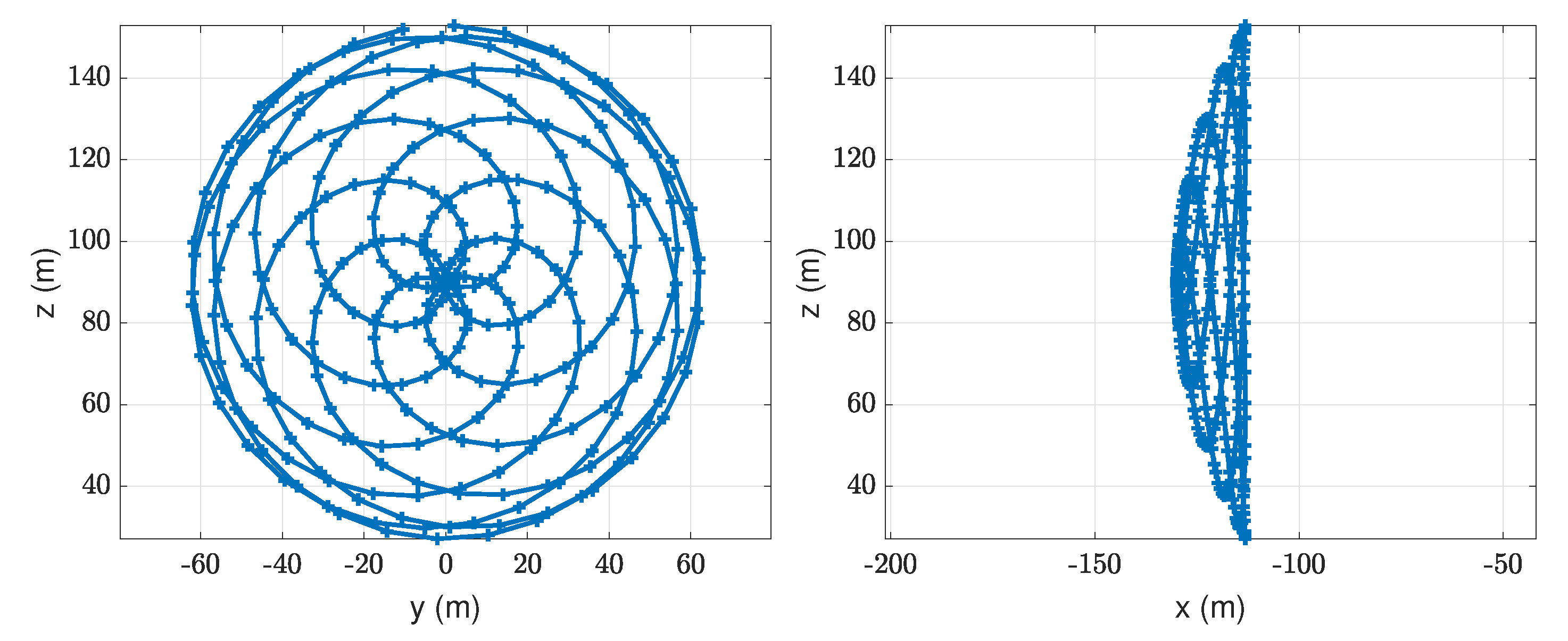
The SpinnerLidar [8,9] is one high-resolution lidar device that satisfies the requirement of fast scanning of the rotor area. This research-based prototype lidar can perform 2D measurements of the radial line-of-sight wind speed on a spherical surface with very high spatial and temporal resolution. The lidar consists of a modified ZephIR-300 continuous-wave Doppler lidar with a 2D scan head developed by the Technical University of Denmark (Figure 1). The scan head consists of two rotating prisms deviating the lidar’s focused beam by an angle of 15 while rotating at a fixed ratio of 7 to 13. The resulting scanning pattern movement creates a fast rosette trajectory covering a large area with a quasi-homogeneous spatial resolution. The lidar can sample up to a maximum of 500 radial line-of-sight measurement points distributed over each completed scan trajectory (Figure 2). The lidar is capable of providing 2D wind field scans at a temporal sampling rate of 1 Hz with a variable focal distance from 10 to 150 m (albeit with a constant opening angle of 30). The probe length is 0.13 or 28.3 m at f = 10 m and f = 150 m, respectively.
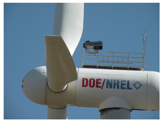
Figure 1.
The SpinnerLidar with its mounting platform mounted on the nacelle of the research turbine CART3 at the National Renewable Energy Laboratory (NREL), Colorado, USA. Photo courtesy of Marijn Floris van Dooren.
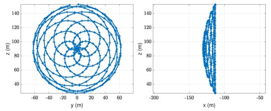
Figure 2.
The rosette scanning pattern of the SpinnerLidar shown from two perpendicular perspectives.
2.4. Large Eddy Simulations (LES) and the Lidar Simulator (LiXim)
Wind turbines operate in the atmospheric boundary layer, which exhibits continuously varying flow characteristics. LES models can accurately resolve the turbulent kinetic energy in the atmosphere, making them suitable candidates for simulating realistic inflow conditions. Therefore, performing virtual lidar simulations inside the LES wind field provides a complete 3D reference wind field for comparison and quality assessment.
The LES data were obtained from simulations with the Parallelised Large Eddy Simulation Model (PALM) revision 3151. The PALM code is widely used for atmospheric boundary layer studies and works by solving the filtered, in-compressible, non-hydrostatic Navier–Stokes equations [38]. PALM employs the Schumann volume averaging approach and uses central differences to discretize the non-hydrostatic and incompressible Boussinesq approximation of the 3D Navier–Stokes equations on a structured Cartesian grid. The simulations presented in this paper were performed using the PALM code in its default settings. The advection terms are solved by a fifth-order Wicker–Skamarock scheme. A third-order Runge–Kutta scheme is applied for the time integration. For cyclic horizontal boundary conditions, an FFT solver of the Poisson equation is used to ensure incompressibility. To model the effects of sub-grid scale turbulence on the resolved scale turbulence, a 1.5th order closure is employed [39]. Monin–Obhukov similarity theory is used to obtain the turbulent fluxes between the surface and the first computational point on the model domain.
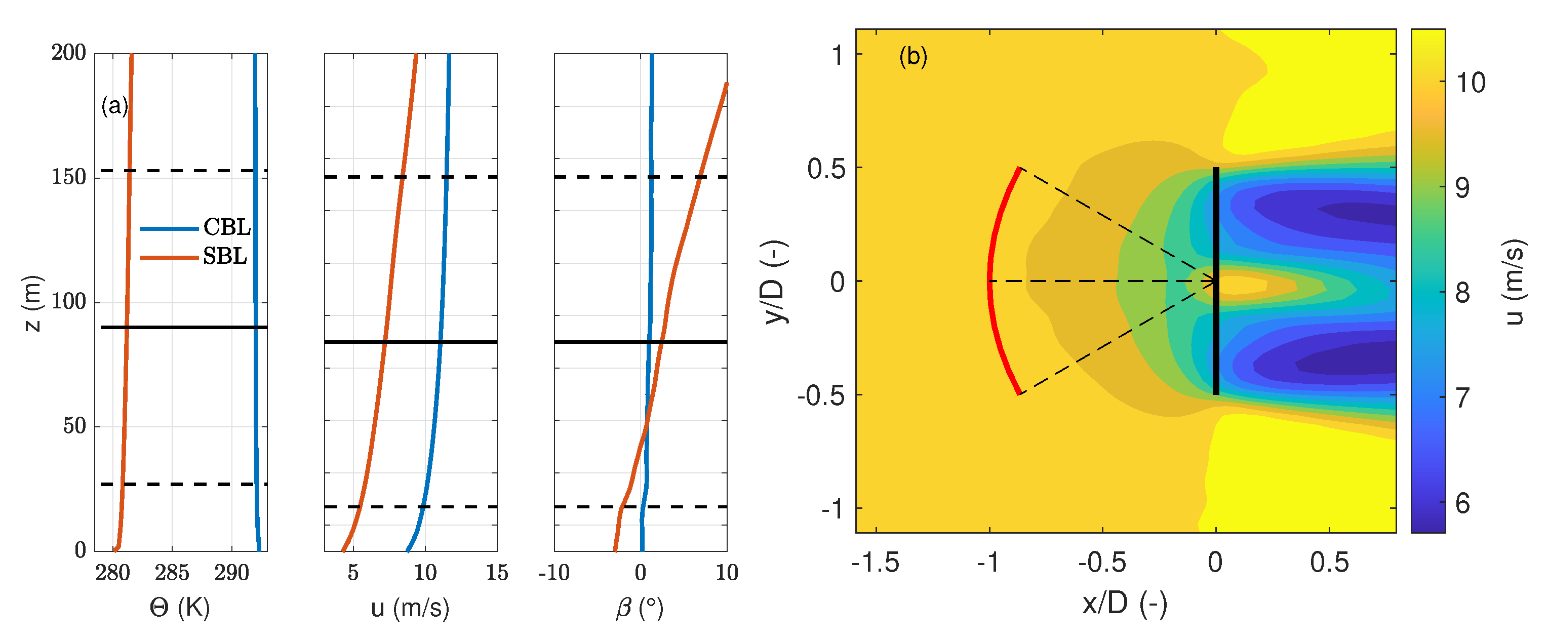
The turbine aeroelastic simulation was performed using the Fatigue, Aerodynamics, Structures and Turbulence code (FAST) v8, developed by the National Renewable Energy Laboratory (NREL) [40]. The code simulates the wind turbine as a combination of rigid and flexible bodies, and the aerodynamic forces are calculated via the AeroDyn module. Both PALM and FAST run simultaneously in an explicit loose two-way coupling [41]. The velocities from the LES field are transferred to FAST, which subsequently calculates the lift and drag on the blade segments based on look-up tables of the airfoil characteristics. Next, the relative velocities of the blades and their new positions are determined. This information is transferred back to PALM, where the forces are distributed back into the flow field, where the induction zone and the wake are generated, as visualised in Figure 3b.
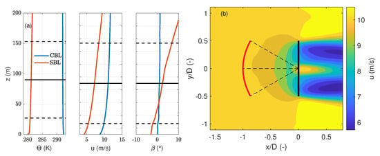
Figure 3.
(a) Vertical profiles of the potential temperature, wind speed and wind veer at the end of the precursor run and (b) the averaged u-component at hub height extracted from the unstable LES wind field for the main run. The black vertical line indicates the position and size of the turbine rotor, and the red curve is the SpinnerLidar’s measurement trajectory.
Two turbulent atmospheric boundary layers (ABL) of unstable and stable stratification, respectively, with a single turbine, were simulated using this framework. The wind turbine model was the actuator line implementation of the NREL 5 MW reference turbine [42] with a rotor diameter of 126 m, a hub height of 90 m and 63 blade sections.
To obtain a convective boundary layer (CBL), we performed a pre-run of 25 h to allow the boundary layer to develop and reach stationary flow. A roughness length m was specified with a friction velocity = 0.52 m/s, and the kinematic sensible heat flux at the surface was fixed at 0.023 K ms. The surface potential temperature was 290 K. The instantaneous fields of the precursor simulation were mapped onto the main simulation via turbulence recycling [43], where the turbine was introduced into the wind field. For simulating stable atmospheric conditions (SBL), a pre-run of 25 h was carried out, where the lowest grid cells were constantly cooled at a rate of 0.25 K/h. A roughness length of m was specified, and a temperature gradient of 1 K/100 m was specified. Similarly to the CBL case, the turbine was introduced in the main run, where the precursor simulation was mapped onto the main simulation. Important details of the precursor and the main run are summarised in Table 1. The dimensions of the simulation domain and were normalised with the rotor diameter of the NREL 5 MW turbine. The mean longitudinal wind speed and turbulence intensity were defined as and , respectively. The wind veer was calculated between the top and bottom rotor tips, and was the vertical shear exponent. was the roughness length, and the stability was characterised by the Obhukov length L.

Table 1.
Setup of the two LES simulations and the results at the end of the precursor run.
To extract the SpinnerLidar measurements from the two LES wind fields, we used the integrated lidar simulation toolbox LiXim (Lidar Scanner Simulator) [44]. The SpinnerLidar was simulated in the LES using the LiXim simulator measuring at a focal distance of 126 m (1D) with a temporal resolution of 1 Hz for a total duration of 3700 s. The lidar simulator emulates the lidar measurements inside the LES wind field while considering the volume averaging effect and producing 312 measurement points distributed along the rosette scan pattern. The lidar simulator freezes the wind field for every measurement point and performs linear interpolation to obtain the projection in the direction of the laser beam. From the lidar properties and the focus distance, the length of the measurement volume is defined. The wind field is then interpolated over this volume, and the wind velocities along the line-of-sight are weighted based on the Lorentzian function. The lidar spatial averaging is described as a Lorentzian function for continuous-wave lidars [35]. The effective probe length in terms of the FWHM of the SpinnerLidar when focused at a measurement range of 126 m (1D) is approximately 19 m. The simulated lidar device was assumed to have a horizontal orientation, and the rotor tilt was not considered. The measurements are then interpolated onto a uniform grid with a 3 m spacing resulting in 1261 grid points.
3. Results
The performances of the POD-based reduced-order reconstructions were tested for virtual scanning lidar in the LES data. The simulations were used as a benchmark for comparing and quantifying the accuracy of the inflow based on various reconstruction metrics, such as the energy distributions, velocity field reconstruction, wind field parameterisation and turbulent spectra in the fixed and rotational frames of reference. Finally, the ability of the Gappy-POD method to reconstruct artificially removed measurement points was investigated for a range of data availabilities.
3.1. Application of the POD Methodology to Scanning Lidar Measurements
The eigenvalues and eigenvectors associated with the covariance matrix for the line-of-sight velocity fields of the two simulations were calculated based on Equation (3).
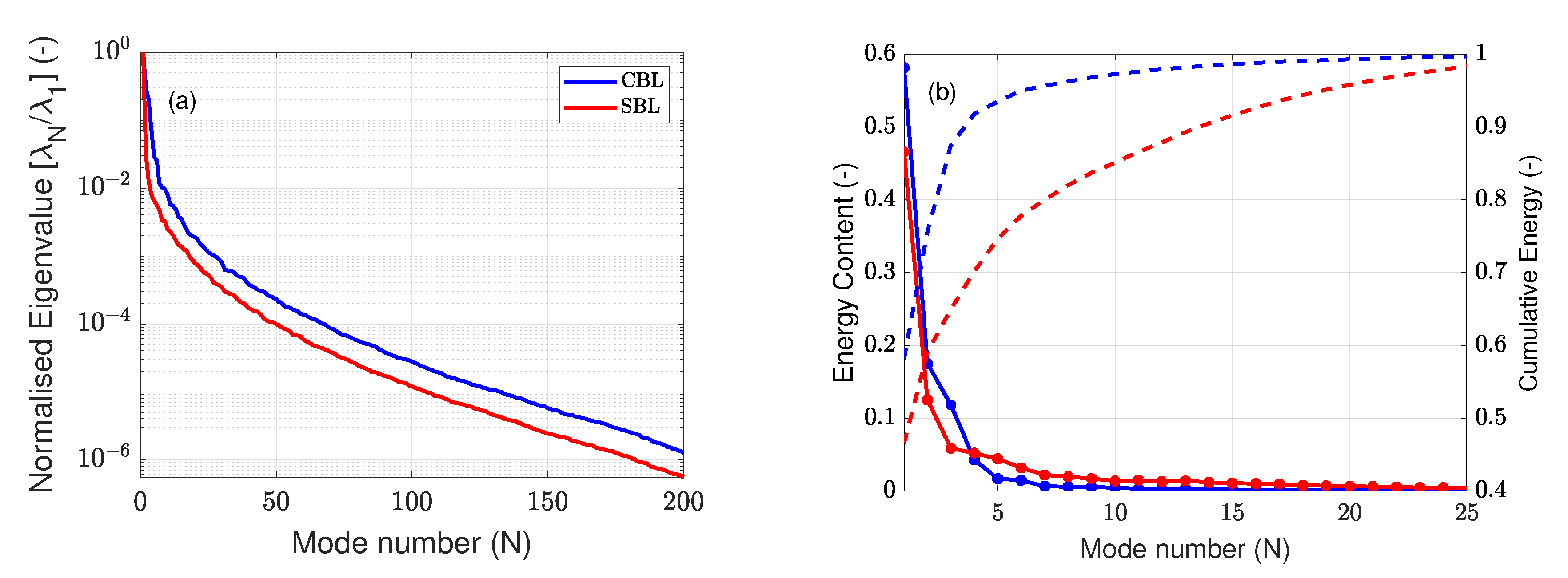
The normalised magnitudes of the eigenvalues and the fraction of energy associated with each mode of the measurements are shown in Figure 4. As expected, the eigenvalue magnitudes of the CBL modes contain more energy in general compared to the SBL modes due to the higher turbulence in the CBL. For the unstable case, the first POD mode contains 57.7% of the total measured energy; and the second, third, and fourth modes contribute 17.3%, 11.8% and 4.3%. For the stable case, the energy contributions of the first modes are 48.01%, 12.91%, 6.07% and 5.38%, respectively. It is clear from Figure 4b that the first ten modes contribute 96.6% and 87.7% of the measured turbulent kinetic energy (TKE); and the first 100 modes account for 99.95% and 99.99% for the CBL and SBL cases, respectively. Note that the total TKE measured by the lidar is not equivalent to that in the wind field due to volume averaging induced turbulence attenuation of the line-of-sight measurements. This may be surprising since, in a turbulent flow, energy is distributed over the different scales and its representation might usually require a large number of modes [45]. However, a lidar system acts as a low-pass filter for small scale turbulence due to its volume averaging property. Hence, the small scale turbulence is filtered out, and an accurate representation of the remaining lidar measured total TKE can be recovered with very few modes.
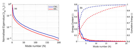
Figure 4.
Eigen value distributions (a) and the energy contribution of each mode (b) for the unstable and stable cases.
The first four POD modes for the CBL and SBL cases are illustrated in Figure 5 and Figure 6, where well defined modes for both cases were obtained. For both cases, the modes exhibit clear structures that trend towards smaller scales with increasing mode number as the modes are sorted based on the energy content, and the kinetic energy decreases with scale. For the CBL case, modes 1 and 2 have similar mode shapes with different gradients, resulting from the variation in the line-of-sight velocities decreasing toward the edges of the scan pattern. The first two modes do not exhibit clear symmetry around the rotor axis due to the slight wind shear present in the ABL. Modes 3 and 4 display variations in the horizontal and vertical directions, respectively. For the SBL case, the first mode shows a strong spatially localised shape related to the line-of-sight velocity distribution, and the second mode resembles a large gradient in the vertical direction, probably due to the strong vertical shear. The third mode displays variations in the horizontal direction, and the fourth mode shows a slightly more complex distribution. The asymmetry of the SBL modes could be explained by the larger surface roughness of the simulation ( m) leading to a large effect of the ground on the inflow. Comparatively, the CBL was generated with less surface roughness ( m), thereby preserving weak statistical isotropy commonly observed in turbulent flows. As expected, the higher mode patterns became increasingly complex compared with the first few modes.

Figure 5.
POD modes 1 to 4 of the line-of-sight () measurements for the CBL case.

Figure 6.
POD modes 1 to 4 of the line-of-sight () measurements for the SBL case.
3.2. Reconstruction of the Reduced Velocity Field
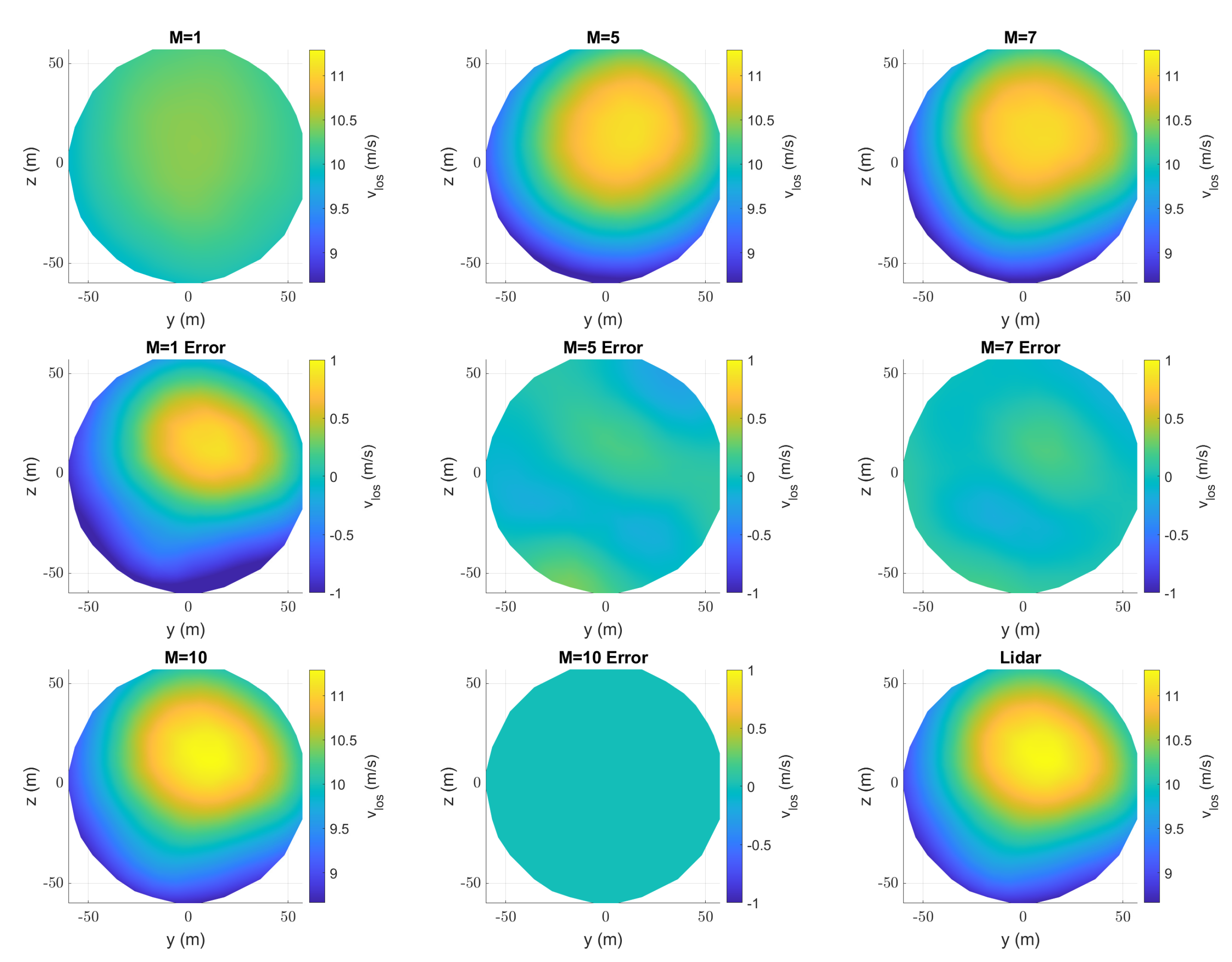
The extracted POD modes were used to reconstruct the velocity field based on Equation (6) by choosing increasing values of M (the number of modes used for reconstruction). A snapshot of the velocity field at an arbitrary time s of the CBL inflow case was reconstructed and illustrated in Figure 7 for a different number of modes, along with its corresponding planar velocity reconstruction error in comparison to full lidar measurements. A more detailed wind field reconstruction was achieved while considering more modes for the reconstruction. For the reconstruction with M = 1 (first mode alone), only the spatial variations in the line-of-sight measurements were obtained, as indicated by a constant velocity distribution over the whole measurement plane, which is also supported by the M = 1 error plot with respect to the full lidar measurements. The addition of more modes into Equation (6) adds more localised wind field information, as the smaller wind field fluctuations which are contributed by the higher modes are taken into account. The velocity field reconstruction with ten modes shows close agreement with the untruncated full lidar measurements; reconstruction error is effectively reduced to almost zero throughout the measurement plane. The high recovery of kinetic energy in the first few modes, as discussed in Section 3.1, indicates that only a few modes are required to create a meaningful reduced-order model capturing all spatial variations in the wind field. For brevity, we only show the results of the CBL case, as the SBL also exhibited the same behaviour: the addition of more modes improving the spatial velocity reconstruction.

Figure 7.
CBL case: Reconstruction of the line-of-sight () velocity snapshot at an arbitrary time instant t = 256 s with different numbers of modes ( and 10) and their corresponding errors with respect to full lidar measurements (bottom right-hand plot captioned as lidar).
3.3. Reconstruction Evaluation Using the Three-Parameter Wind Field Model
The main objective of any inflow sensing lidar is to capture the inflow, along with its variations that significantly impact the wind turbine. Thus, the quality of reconstruction should be evaluated with respect to wind field parameters that directly affect the turbine itself. For example, parameters such as the rotor effective longitudinal wind speed , horizontal misalignment and vertical shear are necessary to implement a standard individual pitch controller. The rotor effective wind speed quantity is related directly to the turbine’s dynamic response and power output. This is the primary variable for selecting the operational condition of the turbine and input for collective pitch control. The horizontal misalignment and vertical shear are essential for for determining the turbine’s yaw setting and individual pitch control algorithms, whereby the controller compensates for asymmetric loading by pitching the blades individually. To extract the wind field parameters from the scanning lidar line-of-sight measurements, we used the three-parameter methodology from Kapp [11]. While the three-parameter methodology can be directly applied to the lidar data to obtain the relevant wind parameters, we calculated them from the reconstructed velocity fields to assess the reconstructed wind field’s accuracy and provide a physical interpretation for the modes.
The three-parameter method proposes a parameterisation of the inflow wind field using three parameters to achieve the smallest possible deviation from the actual inflow field. At every measurement point, the lidar measures the line-of-sight speed as a projection of the 3D wind components, following Equation (11). The measured line-of-sight speeds in the spherical SpinnerLidar measurement plane could be fitted as a set of three parameters that is constant over the whole plane as:
whereas is the unit vector of the laser beam at point i, and and are the Cartesian coordinates of the point in the scanning plane. Grouping every point in the measurement plane results in a set of equations for every measurement point that could be solved in a least-square sense to determine the unknown parameters , :
3.3.1. Time Series Reconstruction of the Three-Parameter Model
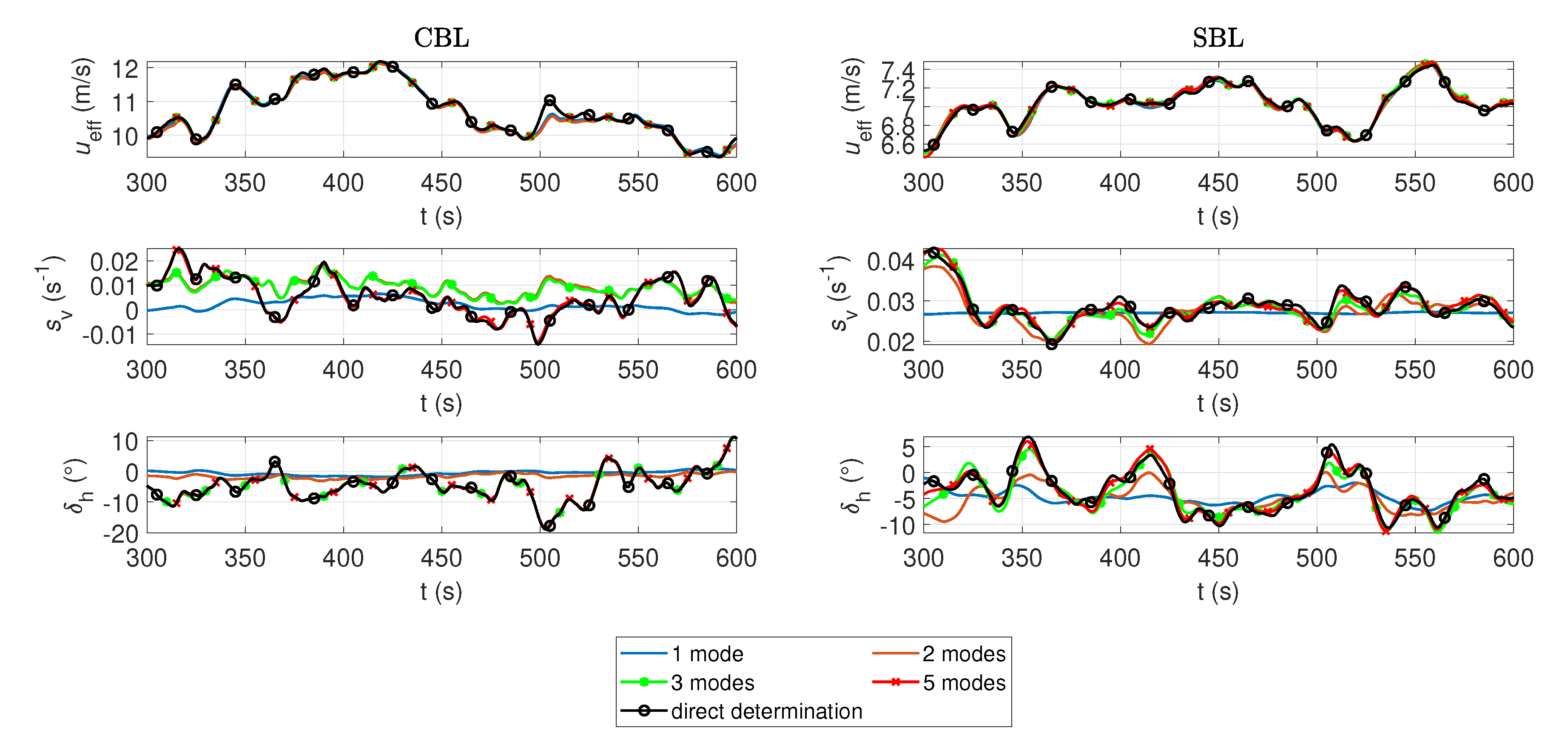
To quantify the reconstruction accuracy, inflow wind field parameters were extracted from the line-of-sight velocity distribution defined in Section 3.3. The results of the extracted wind field parameters from different reconstructions are compared with each other and with the full lidar measurements for the CBL and the SBL inflow cases. The three-parameter wind field model was applied to the SpinnerLidar simulations, which will henceforth be referred to as direct determination. Various reconstructions were created by truncation with M = 1, 2, 3, 5 and 10 modes, and the associated wind field parameters (, and ) were calculated and compared with direct determination. For all the cases and parameters, there were negligible differences between the reconstructions with and , and hence, only the reconstruction with is shown for brevity.
Figure 8 contains part of the time series of the three wind field parameters for different reconstructions with , 2, 3, 5 and 10 for the CBL and SBL cases, respectively. For the rotor effective wind speed , the time series of the different reconstructions overlap with each other well, even for reconstructions with few modes for the CBL and the SBL cases. The dynamic aspects of the rotor effective velocities calculated with different mode numbers are similar, there being only small variations between the reconstructions with and modes. The low-frequency characteristics of the time series were reproduced with reasonable accuracy with just one mode. The addition of more modes to the reconstruction introduced a few high-frequency variations to the time series. However, this was not the case for vertical shear or yaw misalignment. The reconstruction of with one mode for the CBL case showed an average value of zero, whereas for the SBL case a value of 0.025 s was obtained, indicating that the first mode contained some vertical shear information. With the addition of the second and third modes to the reconstruction, we observed that the dynamics of the vertical shear were captured, albeit a little over-predicted for the CBL case. The horizontal misalignment reconstruction for CBL and SBL showed very similar behaviour. With the first mode alone, the basic dynamics of the time series were not captured. The addition of more modes to the reconstruction improved the estimation of both and . For or higher, good agreement between the direct determination and the truncated reconstructions was obtained for all three parameters for both cases.

Figure 8.
The time series of the wind field parameters and extracted at a sampling rate of 1 Hz for a duration of 300 s for different POD reconstructions for the CBL and SBL cases.
3.3.2. Accuracy of the Three-Parameter Wind Field Reconstruction and an Interpretation of the POD Modes
To quantify the reconstruction error associated with these wind field parameters, we write
where is the set of rotor-averaged wind field parameters calculated by applying a three-parameter methodology to the line-of-sight velocities. Similarly, the wind field parameters determined from the reduced-order reconstruction with M modes can be represented as:
The quality of the reconstructed wind field and the corresponding wind field parameter with M modes can be assessed by comparison to the original wind field parameters . To evaluate the reconstruction efficiency, two different error parameters are introduced. The errors associated with the reconstruction of the wind field parameter are defined as:
where and represent the standard and dynamic error, respectively. These values quantify the respective mean error and the error associated with the fluctuations in the wind field. The definition of the dynamic error was motivated by the fluctuation of wind field parameters having the largest effect on the loading and the fatigue of the turbine in contrast to the mean wind field parameters. To investigate the relationship between the POD temporal gains and the wind field parameter time series, the Pearson correlation coefficient is used [46].
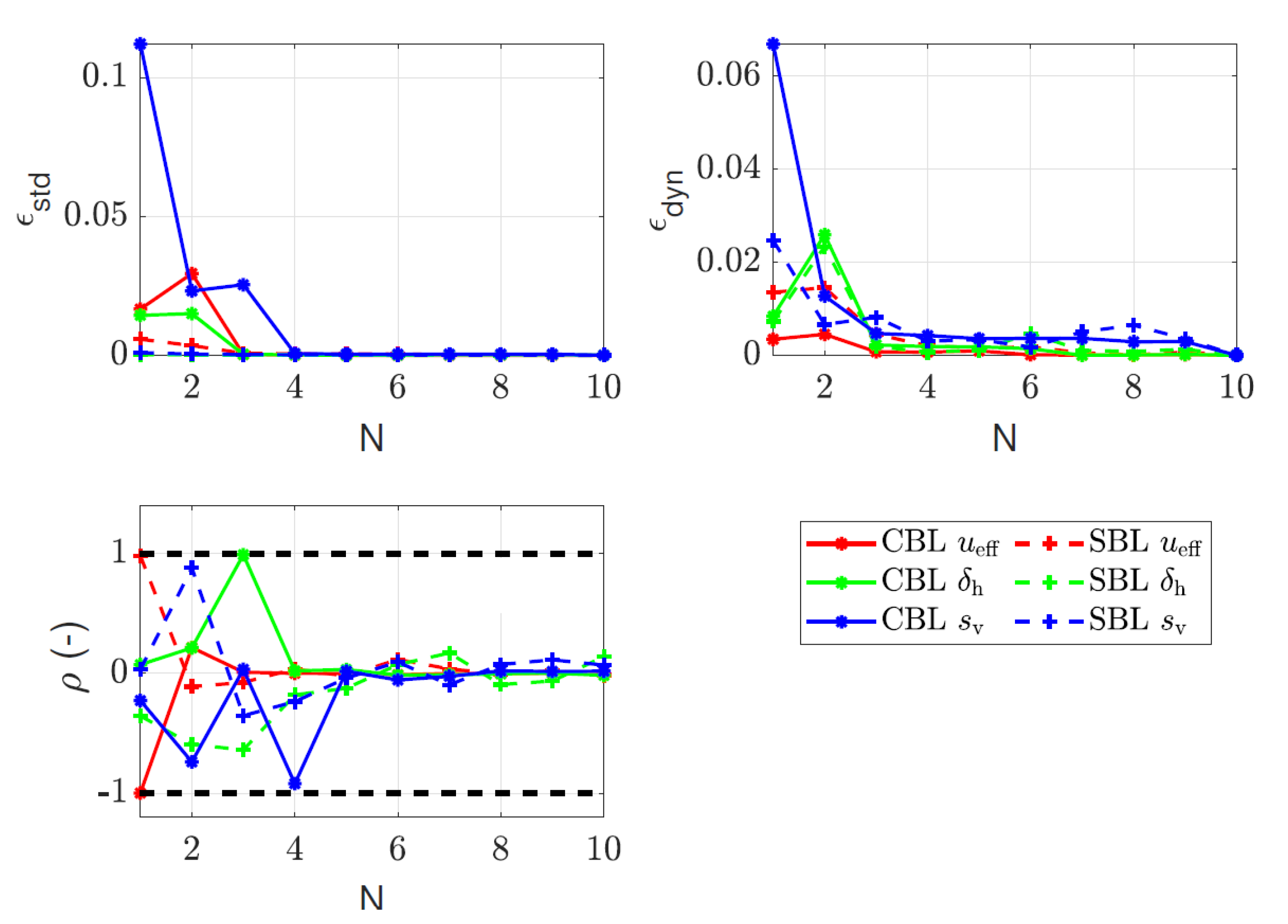
The standard and dynamic errors and were used to quantify the reconstruction quality for the CBL and SBL cases, as depicted in Figure 9. The standard and dynamic errors exhibited similar trends for the CBL and SBL inflow cases. The standard error of reconstructed rotor effective wind speed remained less than 0.016 and 0.005 for the CBL and SBL cases for the reconstruction based on the first mode, indicating the first mode is highly correlated with the rotor averaged wind speed. For both cases, the standard reconstruction errors with one mode for and were comparatively large but dropped when more modes were used. The standard errors for all the three wind field parameters decreased below 0.001 when considering the first five modes for the reconstruction. The standard error exhibited discontinuous behaviour for certain wind field parameters when certain modes were considered. The steep fall in the standard error magnitude with the addition of certain modes indicates that these modes are strongly correlated with these wind field parameters. The dynamic error for dropped below 0.002 for both cases when at least the first three modes were considered for the reconstruction. For both cases, the dynamic error of the three-parameter reconstruction also reduced below 0.001 while considering the first ten modes for reconstruction. Similar discontinuous behaviour was observed while considering specific modes. The discontinuous behaviour shown by the standard and dynamic errors occurring at identical mode numbers indicates a relationship between the particular mode and the corresponding wind field parameter.
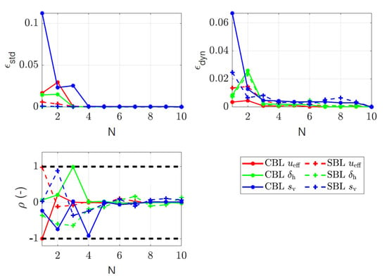
Figure 9.
The standard () and dynamic () errors of the three-parameters calculated for reconstructions with various numbers of modes; correlations () between the time series of the reconstructed three-parameter wind field parameters; and the time evolution of the different POD modes .
The huge reductions in the standard and dynamic errors can be explained by the plots of correlation between the time series of the POD time coefficients and the wind field parameters , as visualised in Figure 9. Confirming the hypothesis for the CBL case based on the time series reconstruction of the rotor effective velocity (Figure 8), the first mode is highly anti-correlated with spatial fluctuations in the wind field with . The yaw misalignment () is related to the third mode with . The vertical shear () is related to the second and the fourth modes and . The argument of the relationship between the wind field parameters and the modes is also strengthened by the shapes of the POD modes (Figure 5): the third and fourth modes exhibit horizontal and vertical structures, whereas the first mode resembles the variations. Similar arguments could be made for the SBL case, as the first mode is highly correlated with the spatial fluctuations in the effective wind speed: . The vertical shear is highly correlated with the second mode, , and weakly anti-correlated with the fourth mode, . The yaw misalignment has the highest correlation with the third mode, , and also exhibits correlations with the first () and second modes (). The second POD mode in Figure 6 exhibits a vertical distribution, and the third POD mode shows a horizontal distribution, further strengthening the argument that the POD modes are related to the properties of the inflow itself.
3.4. Reconstruction Evaluation in the Frequency Domain
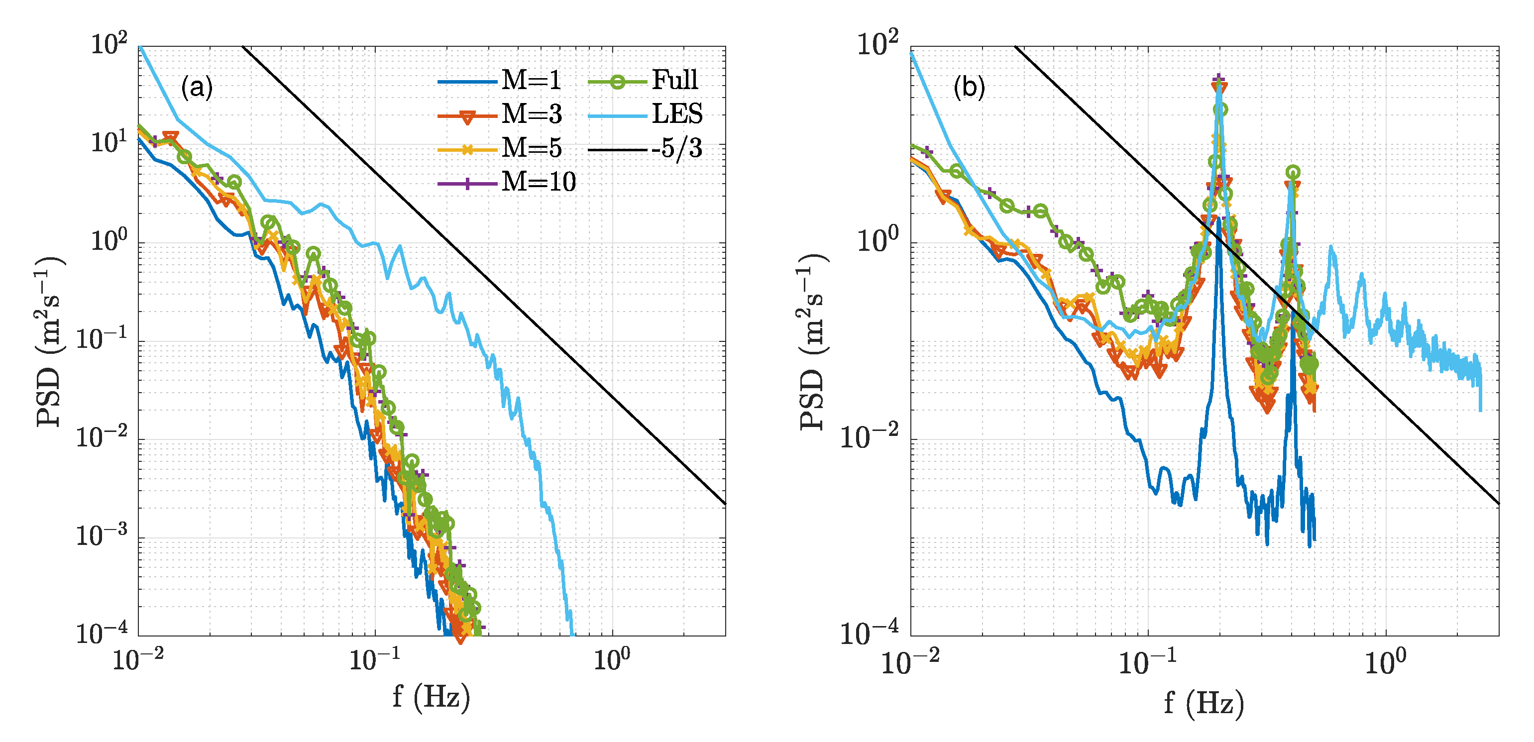
The dynamic loading induced on the turbine blades is determined by the wind fluctuations impinging on the blades and how quickly they rotate. As the blades move through the turbulent wind field, they perform a so-called “rotational sampling” of the turbulent structures, which differs from the velocities observed at a stationary point [47]. To investigate this effect, we calculated the auto-spectral density of the longitudinal wind speed of the reduced-order reconstruction for the stationary hub centre and rotating reference frames for a radial position of 90% on the first blade only for the CBL case. The reconstructed spectra are evaluated with respect to the turbulent spectra directly determined by the lidar measurements and the reference LES (Figure 10).
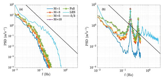
Figure 10.
(a) Fixed point spectra of the velocity on the rotor axis at an upstream measurement distance of 126 m with M = 1, 3, 5 and 10 modes. (b) Rotational spectra of the velocities of the reduced-order reconstruction with M = 1, 3, 5 and 10 modes. The results are shown only for the CBL case.
The spectra were calculated via Welch’s modified periodogram method with a Hanning window, 300 s data segments and a 50% overlap between segments. For the hub centre point visualised in Figure 10a, the spectra of the different reconstructions exhibit very similar behaviour. LES in the figure refers to the spectrum calculated from the reference wind field sampled at 5 Hz, and the Kolmogorov slope is illustrated as a black line. The spectrum directly determined from the full lidar measurements is illustrated by the green line. The lidar measurements for all cases show a drop-off from the Kolmogorov slope at 0.03 Hz, evident of the low-pass filtering effect of the lidar. The reconstructed spectrum with the first mode underpredicts the energy content by one order of magnitude, and the addition of more modes moves the spectrum upwards toward the full lidar measurements. The reconstructed spectra with ten modes and the full lidar measurements show no differences, indicating that with the first ten modes, almost all energy is recovered in comparison to the full lidar measurements.
However, completely different behaviour is observed when examining the rotationally sampled spectra of the projected longitudinal wind speed at an upstream measurement distance of 126 m sampled at 90% of the outer blade radius moving at 11.88 rpm, as shown in Figure 10b. The rotational spectra is calculated from the velocities (by setting in Equation (11), leading to . The light blue line shows the spectrum of the reference LES simulations sampled at 5 Hz. The 1P frequency (0.198 Hz) and the next five peaks of the higher harmonics are clearly visible. The reconstruction with underpredicts and cannot capture the magnitude of the 1P and 2P peak, as the first mode only reconstructs the relatively weak radial asymmetry of the wind speeds over the wind field. With the addition of the second and third modes, the magnitudes of the 1P and 2P peaks are accurately reconstructed; adding more modes leads to marginally better predictions of these rotational harmonics. The higher harmonics seen in the rotational spectrum of the LES curve are not captured by the lidar due to the limited 1 Hz sampling rate yielding a corresponding Nyquist frequency of 0.5 Hz. The superior reconstructions in the rotational spectra in comparison to the fixed point spectra, even for modes, can be attributed to the high spatial coverage of the lidar. Moreover, the fact that the dominating POD modes have clear relationships with the wind speed changes in the horizontal and vertical directions allows for better calculation of the rotational spectrum compared to the fixed frame. Note that the lidar measures more energy than the LES field at lower frequencies due to cross-contamination of the lateral and vertical components contributing to increased variance in the line-of-sight velocity.
3.5. Gappy-POD Reconstruction of Missing Data Points
Here, we present the results of using the Gappy-POD algorithm to reconstruct missing data points. We define total data availability over the entire dataset as the percentage of the average available wind field view allowed by the rotor. Gappiness is defined as:
where denotes cardinality. The removal of points was based on defining a set of uniformly distributed pseudo-random integers consistent with the total number of measurement points using the Mersenne–Twister algorithm [48]. Different gappiness scenarios were created by randomly removing 10%, 20%, 30%, 40% and 50% of the data points from the CBL and SBL cases. Gappy-POD was applied to the gappy datasets, and the ability of the method to reconstruct missing points was evaluated. While removing measurement points, it was made sure that there were no data points with no data and no snapshot that was missing all measurements. Determining the convergence, i.e., the termination point of the iterative process, is necessary to achieve high accuracy. For this purpose, a convergence criterion based on the root mean square error (RMSE) was utilised only at the locations of the missing points; i.e., valid data points were ignored.
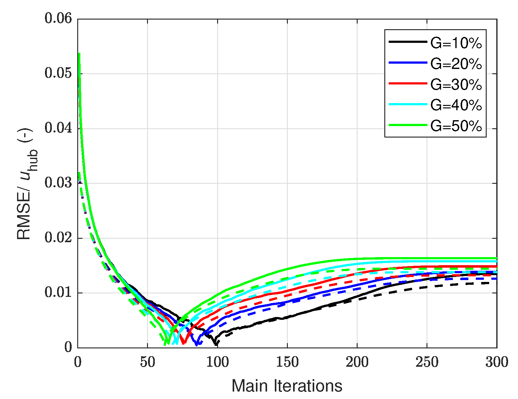
where represents the reconstructed data, represents the reference data with 100% availability and is the number of missing points. The sub-iteration convergence was investigated by inspecting the absolute normalised difference between the eigenvalue spectra between consecutive iterations. In this work, the value was chosen as 0.05. If the convergence criteria was not satisfied, the guess for the missing data was updated using Equation (10) and the next sub-iteration was started. The variations in RMSE with the number of main iterations and for different gappiness G are plotted in Figure 11 for the CBL and SBL cases. The RMSE was normalised by the hub height wind speed to facilitate comparison between the two cases.
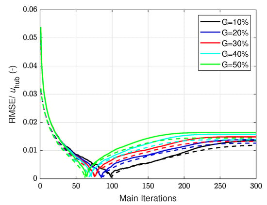
Figure 11.
RMSE normalised with the hub height wind speed as a function of main iterations for the CBL case (solid lines) and the SBL case (dotted lines) for different gappiness percentages.
For all the cases, the normalised RMSE initially decreases, reaches a minimum and starts increasing again, a result of over-fitting. For both cases and all gappiness, the number of main iterations required to reach the minimum RMSE varies, but the optimum is found below 100 iterations. In general, the RMSE drops below 0.01 after 50 iterations for both cases and all availabilities. The SBL case converges slightly earlier and shows slightly reduced RMSE compared to the CBL case, presumably due to the lower turbulence. The motivation for performing the iterative implementation was that the optimum number of iterations for minimum RMSE was unknown. However, if the optimum number is known, the nested-loop algorithm can be modified by just repeating the sub-iterations alone (steps 2 to 4) in Section 2.2, drastically decreasing the required solution time. In the following, we also present the results of the henceforth named "direct Gappy" method, wherein the gappy procedure is performed by using the optimum number of modes obtained from Figure 11.
Figure 12a shows the optimum normalised RMSE of the three methods as functions of G. Here, natural interpolation refers to the C1 continuous triangulation-based natural neighbour interpolation method. As expected, both the direct and iterative gappy methods performed better than natural interpolation; a slight increase in RMSE was noticed with increasing G. The normalised RMSE of the natural interpolation on the CBL case ranged from 0.019 to 0.023; and the normalised RMSE ranged from 0.0008 to 0.0009 and 0.005 to 0.011 for the iterative and direct gappy implementations, respectively. For , commonly observed in full-field measurements, the iterative and direct gappy procedures performed substantially better than spatial interpolation in reconstructing the missing points. In Figure 12b, the time required for the three methods is shown for reconstructing the whole dataset. The spatial interpolation method is the most robust, given solution times of less than 10 s; the solution time for the iterative solver increased with increasing G.The computations were performed based on an un-optimised MATLAB code on a laptop running an Intel i7-4610M processor @ 3 GHz and 16 GB RAM. The iterative gappy solution requires the most processing time due to the time consuming nested loop implementation, whereas the direct gappy procedure is faster by 6 to 14 times depending on the availability. The reduced solution time for the direct gappy procedure is because only sub-iterations need to be performed until eigenvalue convergence, as the optimum number of modes is known.
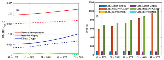
Figure 12.
(a) Error comparison for the three methods. Solid and dotted lines indicate the CBL and SBL cases, respectively. (b) Comparison of the computational time taken for the three methods to reconstruct missing points.
Reconstruction of Spatial Wind Field Parameters
To quantify the accuracy of the reconstructed points, we calculated the wind field parameters (Section 3.3) from the filled wind field for the three methods and compared them against the reference dataset with 100% availability. As the reconstruction of the rotor effective wind speed is trivial for scanning lidars with high spatial resolution, we introduce a spatial turbulence intensity parameter to evaluate the reconstruction. The spatial TI is defined as:
where and are the spatial standard deviation and the mean of the line-of-sight velocities calculated for each snapshot, respectively. The results of the reconstruction are plotted for the CBL case in Figure 13 and the SBL case in Figure 14.

Figure 13.
Comparison of , and calculated from the reconstructed data for the CBL case with .

Figure 14.
Comparison of , and calculated from the reconstructed data for the SBL case with .
For both cases, similar behaviour for the iterative and direct Gappy-POD methods can be observed: both methods perfectly reconstructed the wind parameters and . Spatial interpolation of missing points led to very similar but slightly lower performance for and in comparison to the two Gappy-POD methods. This was expected, as the vertical shear and directional misalignments were averaged over the entire measurement plane, and hence small spatial fluctuations are averaged out. The reconstruction was comparatively poorer for the SBL case: the regression line is characterised by a larger slope in comparison to the reference. However, the spatial TI estimated by interpolation has more scatter and offset in comparison to the reference: and , respectively, for the CBL and SBL cases. The estimated spatial TI of the two gappy methods agree better with the reference. There was almost no difference between the two methods ( 0.99 for both cases).
4. Discussion
We applied the POD methodology to reconstruct scanning lidar measured inflow data from two large eddy simulations of different inflow conditions. The first goal of this work was to apply POD to turbine-mounted scanning lidar measurements of the inflow and to identify the most energetic and dominating modes which can be used to create a reduced-order inflow reconstruction. Secondly, we tackled the problem of blade interference for nacelle-mounted lidars by using two Gappy-POD techniques to fill in missing data points and performed a comparison against spatial interpolation to quantify the reconstruction accuracy.
4.1. Towards POD-Based Reduced-Order Inflow Modelling
The first goal of our work was to identify dominant modes that could yield strong dimensional reduction of the inflow while preserving the spatio-temporal dynamics. After such a dimensional reduction, the application of reduced-order modelling methods to scanning lidar measurements can be performed. Previously, analysis of the reduced-order descriptions of wind turbine inflows and wakes [21,24] focused on the longitudinal velocity component due to its direct impact on the dynamical turbine response. While nacelle-lidar estimations of the longitudinal velocity rely on the dominance of the longitudinal component over the lateral and vertical wind components () in the line-of-sight direction, this is only an approximation with a certain error that depends on the orientation of the inflow in regard to the turbine and the beam direction itself, alongside effects of terrain, atmospheric stability, wind veer and turbine yaw setting. In accordance with our methodology, we did not impose strong wind field assumptions prior to the wind field reconstruction. Therefore, the methodology was applied directly to the line-of-sight measurements rather than projections in the longitudinal direction. Wind field reconstruction methods could be subsequently applied on the reduced line-of-sight wind field to extract wind parameters describing the turbine inflow. While estimating three-component velocity fields from line-of-sight measurements is a challenge in itself [16], a more detailed lower order inflow description could be potentially obtained by including all three velocity components. For quantifying the performance of a reduced-order reconstruction of the inflow, metrics related to the entire wind field were chosen. We see that with the first ten modes, most of the total lidar measured kinetic energy was recovered for both cases characterised by a sharp slope of the eigenvalue distributions (Figure 4). The majority of the lidar measured energy was concentrated in the first few modes, as the energy associated with the small scale turbulence was low-pass filtered due to the lidar volume averaging property. This lidar effect also nullifies the disadvantage of POD, whereby a large number of modes are generally required to capture small turbulent structures.
We observed that the dynamical behaviour of inflow characteristics relevant for turbine-based lidar applications was captured with high accuracy with just a few modes. The reconstruction accuracy further was quantified by calculating wind field parameters commonly used for turbine IPC control. The low-frequency characteristics of the rotor effective wind speed, vertical shear and horizontal misalignment can be captured by the first few modes alone (Figure 8); and the high-frequency fluctuations in the wind field parameters were reconstructed with high accuracy by taking the first ten POD modes. This indicates that simplified reduced-order dynamic models could be developed based on considering these dominant modes alone. Interestingly, the addition of certain modes to the reconstruction reduces the reconstruction errors substantially, suggesting that certain wind field parameters could be related to specific POD modes. From the high correlations between the modal time evolution and the wind parameters (Figure 9), it is clear that certain modes are related to certain wind field characteristics, providing a physical mode interpretation. We acknowledge that the modal interpretations with inflow parameters cannot be generalised and would vary depending on the inflow conditions, as seen from the varying correlation between the two considered LES fields. In addition, the reconstruction of turbulent spectra in fixed and rotating reference frames was investigated (Figure 10). For the stationary hub height spectra, 10-mode reconstruction offers good agreement with the lidar measured spectra. While reconstructing the rotational spectra necessary for modelling periodic blade loads, the eddy slicing effect (1P, 2P harmonics) is captured remarkably accurately with three or more modes.
Creating an inflow reconstruction with POD offers certain advantages over existing WFR methods. This method does not require strong assumptions about the wind field, unlike other WFR methods [11,12]. A POD-based inflow model also provides spatial wind information on a reduced basis, whereas parameterisation models only provide spatially constant wind parameters over the whole measurement plane. Hence, these models do not utilise the high spatial resolutions offered by scanning lidar systems such as SpinnerLidar, and events such as partial wakes and gusts are misinterpreted. Since the typical wind field characteristics for lidar-assisted 1P IPC are based on three parameters only, the effects of local flow details (partial wakes, gusts) are averaged out and are poorly represented in the wind field model. A POD reconstruction can represent significantly more wind field details, and hence can be used even for higher harmonics (e.g., 2P) in IPC or trailing edge flap control [49]. This would make a POD-based inflow model attractive for wind turbine control, as the dynamics of the non-homogeneous inflow can be described with a few modes and their weighing coefficients.
Creating a reduced-order dynamic inflow model can be achieved by Galerkin projection of the dominant POD modes onto the underlying Navier–Stokes equations governing the flow [20] or modelling the temporal dynamics of the weighing coefficients as a stochastic process [50], or by linearising the temporal dynamics of the weighing coefficients [51,52]. As wind turbines operate under conditions characterised by continuously changing states, special considerations must be given to dynamically adapt the ROM to changes in inflow states. This can be achieved either by determining the POD modes from a large dataset covering the majority of the inflow states, or by dynamically adapting the reduced-order model with state changes [53,54,55,56,57].
To date, we have only investigated the quality of the reduced-order descriptions of the inflow dynamics based on two LES simulations. A general statement on the factors influencing our results cannot be derived without analysing a large enough dataset that considers variations in wind, atmospheric conditions and rotor sizes covering a variety of inflow and stability conditions that a turbine might experience during its lifetime. However, our simulations of two cases of typical atmospheric stratifications indicate that the majority of the energy was concentrated in the first ten dominant POD modes, and similar results were seen in free-field data as well. As most of the spectral energy in the flow are concentrated in the larger scales [58], the spatio-temporal flow variations would be captured in the first dominant POD modes, and the smaller scale structures would be filtered out due to the low-pass filtering of the measurements themselves. The effects of the larger scanning areas required for larger turbines and the representation of large atmospheric structures should be further analysed. However, for such an analysis, the optical parameters of the scanning lidar need to be modified to increase the measurement range and decrease the probe volume at large focal distances. As previously mentioned, the quality of the wind field reconstruction depends directly upon the lidar data quality and is thus subject to inaccuracies caused by the device’s limitations. These shortcomings which are inherent device properties must be investigated in detail concerning their potential lidar-based relevance. In this study, the metrics for quantifying the accuracy of the model were chosen based on the inflow wind field itself. To further investigate the relationship between lidar measured wind fields and turbine dynamics, a detailed evaluation of the POD model could be performed by choosing quantities that describe the turbine’s response.
4.2. Reconstruction of Missing Data Points Using Gappy-POD
We used Gappy-POD to reconstruct missing data points removed artificially to simulate blade interference. Gappy-POD utilises POD modes as a basis for the reconstruction of missing data points. The convergence of Gappy-POD was quantified using the root mean square error at the reconstructed points at every main iteration. Even up to a randomised gappiness of 50%, the RMSE dropped below 0.1% between 50 and 100 iterations. The Gappy-POD reconstruction algorithm was capable of reconstructing up to 50% missing data considerably better than spatial interpolation. This is because the spatio-temporal variations in the wind field are considered by Gappy-POD, whereas interpolation only uses the spatial information at neighbouring valid points. The reconstructed parameters with Gappy-POD agree better with the reference compared to spatial interpolation (Figure 13 and Figure 14). To reduce solution times, a modified version of the Gappy-POD algorithm was presented where the iterative algorithm is replaced by direct solving using the optimum number of iterations (Figure 12). The direct Gappy implementation was able to achieve similar performance in reconstructing wind field parameters, with a 6 to 14 times reduction in solution times, depending on availability. However, the optimal number of modes required for reconstruction should be known in advance. Performing the direct calculations in a high-level programming language could reduce solution times to a few seconds, thereby making real-time reconstruction of missing points from wind fields possible. As the proposed method requires the time series of lidar measurements to estimate POD modes and iteratively reconstruct data points, a real-time implementation could be challenging. However, real-time reconstruction can be performed by estimating POD modes in an offline stage, which can be then subsequently used to reconstruct sparse data [59]. In [31], it is shown that Gappy-POD would succeed even with random initial guesses but would require more iterations before arriving at a converged solution.
Before performing Gappy-POD, it is necessary that a robust outlier filter is applied to the dataset to detect blade interference and bad quality data due to environmental factors. As Gappy-POD is a data-driven method, the presence of invalid data points would introduce reconstruction errors which would propagate with every main or sub-iteration. It is also important to consider that by performing reconstruction based on lidar measured data, the missing point estimate would be optimised using the measured values. Hence, the reconstructed points will acquire at least the experimental uncertainty of the measurement data themselves [60]. For evaluating convergence in real experimental data, artificial convergence checking gaps can be introduced to the gappy data, over which the reconstruction error can be evaluated [29].
5. Conclusions
Turbine-mounted lidar measurements can be used to derive information about the inflow to the wind turbine, which can subsequently be used for turbine control, load validation or turbulence characterisation. As lidar capabilities improve due to enhanced hardware and larger datasets, it is crucial to reduce the measurement data to a few variables that can still capture the spatio-temporal dynamics of the wind field. Here, we suggested a wind field reconstruction methodology for inflow measurements by a turbine-mounted scanning lidar, based on proper orthogonal decomposition (POD). It was tested in two LES wind fields with different stratifications. Well defined inflow modes were obtained, and the majority of the lidar measured turbulent kinetic energy was captured with just the first ten POD modes for both cases. The data reduction was possible due to the volume averaging effect of the lidar filtering out smaller turbulent structures, thereby taking advantage of one of the lidar’s limitations. The reconstructed velocity fields with the dominant modes agree well with the full lidar measurements and provide a method for extracting local spatial structures in the inflow. The strong dimensional reduction and relationships between wind inflow parameters indicate that the development of simplified inflow models is possible. POD-based wind field reconstruction provides more information than classical methods; for instance, it captures the rotationally sampled wind field and the associated first and second harmonics, which dominate the dynamic blade loading. Furthermore, we used two Gappy-POD methods to fill in measurements lost due to blade passage and other factors that influence data availability, a significant problem for all nacelle-mounted lidars. Gappy-POD provides very good approximations with which to reconstruct data points lost to blade interference and other factors. Both Gappy-POD methods were found to reconstruct the missing data (up to 50%) with high accuracy in comparison to spatial interpolation, as spatio-temporal flow variations are taken into account. The wind field reconstruction method introduced applies to other scanning lidar systems with sufficiently high spatio-temporal resolution.
Author Contributions
A.P.K.S. designed the research, developed the methodology, performed the LES simulations, performed the data analysis and wrote the paper. M.F.v.D. developed the analysis toolbox for the SpinnerLidar together with A.P.K.S., implemented the three-parameter WFR method and thoroughly reviewed the manuscript. A.R. and M.K. contributed with intensive discussions on the scientific content and thoroughly reviewed the manuscript. M.K. supervised the research. All authors have read and agreed to the published version of the manuscript.
Funding
The research was carried out in the framework of the “DFWind” (Deutsche Forschungplattform für Windenergie) project funded by the German Federal Ministry for Economic Affairs and Energy (BMWi) based on a decision of the German Bundestag (grant number 0325936C).
Data Availability Statement
The data of the LES simulations can be made available on request.
Acknowledgments
We acknowledge the help of Sonja Krüger and Gerald Steinfeld in setting up the LES simulations and David Bastine regarding the POD method.
Conflicts of Interest
The authors declare no conflict of interest.
Abbreviations
The following abbreviations are used in this manuscript:
| ABL | Atmospheric Boundary Layer |
| CBL | Convective Boundary Layer |
| FAST | Fatigue, Aerodynamics, Structures and Turbulence code |
| FFT | Fast Fourier Transform |
| IPC | Individual Pitch Control |
| LES | Large Eddy Simulations |
| LiXim | Lidar Scanner Simulator |
| PALM | Parallelised Large Eddy Simulation Model |
| POD | Proper Orthogonal Decomposition |
| RMSE | Root Mean Square Error |
| ROM | Reduced-Order Model |
| SBL | Stable Boundary Layer |
| WFR | Wind Field Reconstruction |
| Symbols | |
| Wind shear exponent | |
| Wind veer (°) | |
| Half Width Half Maximum (m) | |
| Lidar elevation angle (°) | |
| Lidar estimated yaw misalignment (°) | |
| Reconstruction errors | |
| POD eigenvalues | |
| POD spatial mode | |
| Lidar azimuth angle (°) | |
| Blade rotational speed (rpm) | |
| D | Rotor diameter |
| G | Gappiness |
| L | Obhukov length (m) |
| M | Dimensions of the reduced-order reconstructions |
| N | Dimensions of the full reconstructions |
| n | Gappy-POD main iteration indices |
| Unit vector in the beam direction | |
| R | Covariance matrix |
| Lidar estimated vertical shear () | |
| s | Gappy-POD sub-iteration indices |
| TI | Turbulence intensity |
| Projected longitudinal wind speed (m/s) | |
| Hub height wind speed (m/s) | |
| Lidar estimated rotor effective longitudinal wind speed (m/s) | |
| V | Velocity snapshot matrix (m/s) |
| Fluctuating velocity field (m/s) | |
| Filled wind field (m/s) | |
| POD approximation of filled wind field (m/s) | |
| Gappy-POD reconstructed wind field at the end of iteration (m/s) | |
| Time averaged spatial velocity field (m/s) | |
| Converged Gappy-POD reconstruction | |
| Reference Gappy-POD reconstruction | |
| Line-of-sight velocity (m/s) | |
| Fitted line-of-sight of the three-parameter model (m/s) | |
| Location of valid measurement points | |
| Location of invalid points | |
| Friction velocity (m/s) | |
| Modal temporal evolution |
References
- Rettenmeier, A.; Martin, K.; Schlipf, D.; Kapp, S.; Anger, J.; Bischoff, O.; Hofs, M.; Hofsäß, M.; Kühn, M.; Rettenmeier, A.; et al. Prospects of Optimization of Energy Production by LIDAR Assisted Control of Wind Turbines. In Proceedings of the EWEA 2011 Conference Proceedings, Brussels, Belgium, 14–17 March 2011; pp. 1–10. [Google Scholar]
- Simley, E.; Fürst, H.; Haizmann, F.; Schlipf, D. Optimizing lidars for wind turbine control applications-Results from the IEA Wind Task 32 workshop. Remote Sens. 2018, 10, 863. [Google Scholar] [CrossRef] [Green Version]
- Dimitrov, N.; Borraccino, A.; Peña, A.; Natarajan, A.; Mann, J. Wind turbine load validation using lidar-based wind retrievals. Wind Energy 2019, 22, 1512–1533. [Google Scholar] [CrossRef]
- Conti, D.; Dimitrov, N.; Pena, A.; Herges, T. Probabilistic estimation of the Dynamic Wake Meandering model parameters using SpinnerLidar-derived wake characteristics. Wind Energy Sci. 2021, 6, 1117–1142. [Google Scholar] [CrossRef]
- Penã, A.; Mann, J.; Dimitrov, N. Turbulence characterization from a forward-looking nacelle lidar. Wind Energy Sci. 2017, 2, 133–152. [Google Scholar] [CrossRef] [Green Version]
- Held, D.P.; Mann, J. Lidar estimation of rotor-effective wind speed—An experimental comparison. Wind Energy Sci. 2019, 4, 421–438. [Google Scholar] [CrossRef] [Green Version]
- Borraccino, A.; Schlipf, D.; Haizmann, F.; Wagner, R. Wind field reconstruction from nacelle-mounted lidar short-range measurements. Wind Energy Sci. 2017, 2, 269–283. [Google Scholar] [CrossRef] [Green Version]
- Herges, T.G.; Maniaci, D.C.; Naughton, B.T.; Mikkelsen, T.; Sjöholm, M. High resolution wind turbine wake measurements with a scanning lidar. J. Phys. Conf. Ser. 2017, 854, 012021. [Google Scholar] [CrossRef] [Green Version]
- Mikkelsen, T.; Angelou, N.; Hansen, K.; Sjöholm, M.; Harris, M.; Slinger, C.; Hadley, P.; Scullion, R.; Ellis, G.; Vives, G. A spinner-integrated wind lidar for enhanced wind turbine control. Wind Energy 2013, 16, 625–643. [Google Scholar] [CrossRef] [Green Version]
- Wentzel, D.G. On the spectrum of turbulence. In Physics of Fluids; The Royal Society: London, UK, 1958; Volume 1, pp. 213–214. [Google Scholar] [CrossRef]
- Kapp, S. Lidar Based Reconstruction of Wind Fields Additionally, Applications for Wind Turbine Control. Ph.D. Thesis, Carl von Ossietzky Universität Oldenburg, Oldenburg, Germany, 2017. [Google Scholar]
- Raach, S.; Schlipf, D.; Haizmann, F.; Cheng, P.W. Three dimensional dynamic model based wind field reconstruction from lidar data. J. Phys. Conf. Ser. 2014, 524, 12005. [Google Scholar] [CrossRef] [Green Version]
- Schlipf, D.; Rettenmeier, A.; Haizmann, F.; Hofsass, M.; Courtney, M.; Cheng, P.W. Model based wind vector field reconstruction from lidar data. In Proceedings of the 11th German Wind Energy Conference DEWEK 2012, Bremen, Germany, 7–8 November 2012. [Google Scholar] [CrossRef]
- Scholbrock, A.; Fleming, P.; Fingersh, L.; Wright, A.; Schlipf, D.; Haizmann, F.; Belen, F. Field Testing LIDAR-Based Feed-Forward Controls on the NREL Controls Advanced Research Turbine. In Proceedings of the 51st AIAA Aerospace Sciences Meeting including the New Horizons Forum and Aerospace Exposition, Grapevine, TX, USA, 7–10 January 2013; IEEE, American Institute of Aeronautics and Astronautics: Reston, VA, USA, 2013; Volume 2, pp. 5–28. [Google Scholar] [CrossRef] [Green Version]
- Guillemin, F.; Nguyen, H.N.; Sabiron, G.; Di Domenico, D.; Boquet, M. Real-time three dimensional wind field reconstruction from nacelle LiDAR measurements. J. Phys. Conf. Ser. 2018, 1037, 032037. [Google Scholar] [CrossRef]
- Sekar, A.P.K.; Van Dooren, M.F.; Mikkelsen, T.; Sjöholm, M.; Astrup, P.; Kühn, M. Evaluation of the LINCOM wind field reconstruction method with simulations and full-scale measurements. J. Phys. Conf. Ser. 2018, 1037, 52008. [Google Scholar] [CrossRef]
- Berkooz, G.; Holmes, P.; Lumley, J.L. The proper orthogonal, decomposition in the analysis of turbulent flows. Annu. Rev. Fluid Mech. 1993, 25, 539–575. [Google Scholar] [CrossRef]
- Holmes, P.; Lumley, J.L.; Berkooz, G.; Rowley, C.W. Turbulence, Coherent Structures, Dynamical Systems and Symmetry, 2nd ed.; Cambridge Monographs on Mechanics; Cambridge University Press: Cambridge, UK, 2012. [Google Scholar] [CrossRef]
- Sirovich, L. Turbulence and the dynamics of coherent structures. I. Coherent structures. Q. Appl. Math. 1987, 45, 561–571. [Google Scholar] [CrossRef] [Green Version]
- Taira, K.; Brunton, S.L.; Dawson, S.T.; Rowley, C.W.; Colonius, T.; McKeon, B.J.; Schmidt, O.T.; Gordeyev, S.; Theofilis, V.; Ukeiley, L.S. Modal analysis of fluid flows: An overview. AIAA J. 2017, 55, 4013–4041. [Google Scholar] [CrossRef] [Green Version]
- Bastine, D.; Witha, B.; Wächter, M.; Peinke, J. Towards a simplified dynamic wake model using POD analysis. Energies 2015, 8, 895–920. [Google Scholar] [CrossRef] [Green Version]
- Andersen, S.J.; Sørensen, J.N.; Mikkelsen, R.F. Turbulence and entrainment length scales in large wind farms. Philos. Trans. R. Soc. Math. Phys. Eng. Sci. 2017, 375, 20160107. [Google Scholar] [CrossRef] [Green Version]
- Bastankhah, M.; Porte-Agel, F. Wind tunnel study of the wind turbine interaction with a boundary-layer flow: Upwind region, turbine performance, and wake region. Phys. Fluids 2017, 29, 065105. [Google Scholar] [CrossRef]
- Saranyasoontorn, K.; Manuel, L. Low-dimensional representations of inflow turbulence and wind turbine response using Proper Orthogonal Decomposition. J. Sol. Energy Eng. Trans. ASME 2005, 127, 553–562. [Google Scholar] [CrossRef] [Green Version]
- Davoust, S.; Jehu, A.; Bouillet, M.; Bardon, M.; Vercherin, B.; Scholbrock, A.K.; Fleming, P.A.; Wright, A.D. Assessment and Optimization of Lidar Measurement Availability for Wind Turbine Control; Technical Report May; No. NREL/CP-5000-61332; National Renewable Energy Lab. (NREL): Golden, CO, USA, 2014. [Google Scholar]
- Everson, R.; Sirovich, L. Karhunen–Loève procedure for gappy data. J. Opt. Soc. Am. A 1995, 12, 1657. [Google Scholar] [CrossRef] [Green Version]
- Saini, P.; Arndt, C.M.; Steinberg, A.M. Development and evaluation of gappy-POD as a data reconstruction technique for noisy PIV measurements in gas turbine combustors. Exp. Fluids 2016, 57, 122. [Google Scholar] [CrossRef] [Green Version]
- Raben, S.G.; Charonko, J.J.; Vlachos, P.P. Adaptive gappy proper orthogonal decomposition for particle image velocimetry data reconstruction. Meas. Sci. Technol. 2012, 23, 025303. [Google Scholar] [CrossRef]
- Gunes, H.; Sirisup, S.; Karniadakis, G.E. Gappy data: To Krig or not to Krig? J. Comput. Phys. 2006, 212, 358–382. [Google Scholar] [CrossRef] [Green Version]
- Willcox, K. Unsteady flow sensing and estimation via the gappy proper orthogonal decomposition. Comput. Fluids 2006, 35, 208–226. [Google Scholar] [CrossRef] [Green Version]
- Venturi, D.; Karniadakis, G.E. Gappy data and reconstruction procedures for flow past a cylinder. J. Fluid Mech. 2004, 519, 315–336. [Google Scholar] [CrossRef] [Green Version]
- Oliver, M.A.; Webster, R. Kriging: A method of interpolation for geographical information systems. Int. J. Geogr. Inf. Syst. 1990, 4, 313–332. [Google Scholar] [CrossRef]
- Simley, E.; Pao, L.Y.; Frehlich, R.; Jonkman, B.; Kelley, N. Analysis of light detection and ranging wind speed measurements for wind turbine control. Wind Energy 2014, 17, 413–433. [Google Scholar] [CrossRef]
- Kapp, S.; Kühn, M. A five-parameter wind field estimation method based on spherical upwind lidar measurements. J. Phys. Conf. Ser. 2014, 555, 12112. [Google Scholar] [CrossRef] [Green Version]
- Sjöholm, M.; Mikkelsen, T.; Mann, J.; Enevoldsen, K.; Courtney, M. Spatial averaging-effects on turbulence measured by a continuous-wave coherent lidar. Meteorol. Z. 2009, 18, 281–287. [Google Scholar] [CrossRef]
- Mann, J.; Cariou, J.P.C.; Parmentier, R.M.; Wagner, R.; Lindelöw, P.; Sjöholm, M.; Enevoldsen, K. Comparison of 3D turbulence measurements using three staring wind lidars and a sonic anemometer. Meteorol. Z. 2009, 18, 135–140. [Google Scholar] [CrossRef]
- van Dooren, M.F. Doppler Lidar Inflow Measurements. In Handbook of Wind Energy Aerodynamics; Springer: Berlin/Heidelberg, Germany, 2021; pp. 1–34. [Google Scholar] [CrossRef]
- Maronga, B.; Gryschka, M.; Heinze, R.; Hoffmann, F.; Kanani-Sühring, F.; Keck, M.; Ketelsen, K.; Letzel, M.O.; Sühring, M.; Raasch, S. The Parallelized Large-Eddy Simulation Model (PALM) version 4.0 for atmospheric and oceanic flows: Model formulation, recent developments, and future perspectives. Geosci. Model Dev. 2015, 8, 2515–2551. [Google Scholar] [CrossRef] [Green Version]
- Deardorff, J.W. Stratocumulus-capped mixed layers derived from a three-dimensional model. Bound.-Layer Meteorol. 1980, 18, 495–527. [Google Scholar] [CrossRef]
- Jonkman, J.M.; Buhl, M.L., Jr. FAST User’s Guide; Technical Report No. NREL/EL-500-38230; National Renewable Energy Laboratory: Golden, CO, USA, 2005. [Google Scholar]
- Krüger, S.; Steinfeld, G.; Kraft, M.; Lukassen, L.J. Validation of a coupled atmospheric–aeroelastic model system for wind turbine power and load calculations. Wind Energy Sci. 2022, 7, 323–344. [Google Scholar] [CrossRef]
- Jonkman, J.; Butterfield, S.; Musial, W.; Scott, G. Definition of a 5-MW Reference Wind Turbine for Offshore System Development; Technical Report February; National Renewable Energy Lab. (NREL): Golden, CO, USA, 2009. [Google Scholar]
- Lund, T.S.; Wu, X.; Squires, K.D. Generation of Turbulent Inflow Data for Spatially-Developing Boundary Layer Simulations. J. Comput. Phys. 1998, 140, 233–258. [Google Scholar] [CrossRef] [Green Version]
- Trabucchi, D. Lidar Measurements and Engineering Modelling of Wind Turbine Wakes. Ph.D. Thesis, Carl von Ossietzky Universitat Oldenburg, Oldenburg, Germany, 2020. [Google Scholar]
- Bauweraerts, P.; Meyers, J. Study of the energy convergence of the Karhunen-Loeve decomposition applied to the large-eddy simulation of a high-Reynolds-number pressure-driven boundary layer. Phys. Rev. Fluids 2020, 5, 114603. [Google Scholar] [CrossRef]
- Benesty, J.; Chen, J.; Huang, Y.; Cohen, I. Pearson Correlation Coefficient; Springer: Berlin/Heidelberg, Germany, 2009; pp. 1–4. [Google Scholar] [CrossRef]
- Kristensen, L.; Frandsen, S. Model for power spectra of the blade of a wind turbine measured from the moving frame of reference. J. Wind. Eng. Ind. Aerodyn. 1982, 10, 249–262. [Google Scholar] [CrossRef]
- Matsumoto, M.; Nishimura, T. Mersenne twister. ACM Trans. Model. Comput. Simul. 1998, 8, 3–30. [Google Scholar] [CrossRef] [Green Version]
- Ungurán, R.; Petrović, V.; Pao, L.Y.; Kühn, M. Uncertainty identification of blade-mounted lidar-based inflow wind speed measurements for robust feedback-feedforward control synthesis. Wind Energy Sci. 2019, 4, 677–692. [Google Scholar] [CrossRef] [Green Version]
- Bastine, D.; Vollmer, L.; Wächter, M.; Peinke, J. Stochastic wake modelling based on POD analysis. Energies 2018, 11, 612. [Google Scholar] [CrossRef] [Green Version]
- Iungo, G.V.; Santoni-Ortiz, C.; Abkar, M.; Porté-Agel, F.; Rotea, M.A.; Leonardi, S. Data-driven Reduced Order Model for prediction of wind turbine wakes. J. Phys. Conf. Ser. 2015, 625, 012009. [Google Scholar] [CrossRef]
- Debnath, M.; Santoni, C.; Leonardi, S.; Iungo, G.V. Towards reduced order modelling for predicting the dynamics of coherent vorticity structures within wind turbine wakes. Philos. Trans. R. Soc. A Math. Phys. Eng. Sci. 2017, 375, 20160108. [Google Scholar] [CrossRef]
- Bergmann, M.; Cordier, L.; Brancher, J.P. Optimal rotary control of the cylinder wake using proper orthogonal decomposition reduced-order model. Phys. Fluids 2005, 17, 097101. [Google Scholar] [CrossRef]
- Tadmor, G.; Oliver, L.; Noack, B.R.; Cordier, L.; Delville, J.; Bonnet, J.P.; Morzyński, M. Reduced-order models for closed-loop wake control. Philos. Trans. R. Soc. A Math. Phys. Eng. Sci. 2011, 369, 1513–1524. [Google Scholar] [CrossRef]
- Tallet, A.; Allery, C.; Leblond, C. Optimal flow control using a POD-based reduced-order model. Numer. Heat Transf. Part B Fundam. 2016, 70, 1–24. [Google Scholar] [CrossRef]
- Guo, M.; Hesthaven, J.S. Data-driven reduced order modeling for time-dependent problems. Comput. Methods Appl. Mech. Eng. 2019, 345, 75–99. [Google Scholar] [CrossRef]
- Peherstorfer, B.; Willcox, K. Dynamic data-driven reduced-order models. Comput. Methods Appl. Mech. Eng. 2015, 291, 21–41. [Google Scholar] [CrossRef]
- Vollmer, L.; Steinfeld, G.; Heinemann, D.; Kühn, M. Estimating the ake deflection donstream of a ind turbine in different atmospheric stabilities: An les study. Wind Energy Sci. 2016, 1, 129–141. [Google Scholar] [CrossRef] [Green Version]
- Tong, Z.; Li, Y. Real-Time Reconstruction of Contaminant Dispersion from Sparse Sensor Observations with Gappy POD Method. Energies 2020, 13, 1956. [Google Scholar] [CrossRef] [Green Version]
- Murray, N.E.; Seiner, J.M. The effects of Gappy POD on higher-order turbulence quantities. In Proceedings of the 46th AIAA Aerospace Sciences Meeting and Exhibit, Reno, NV, USA, 7–10 January 2008. [Google Scholar] [CrossRef]
Publisher’s Note: MDPI stays neutral with regard to jurisdictional claims in published maps and institutional affiliations. |
© 2022 by the authors. Licensee MDPI, Basel, Switzerland. This article is an open access article distributed under the terms and conditions of the Creative Commons Attribution (CC BY) license (https://creativecommons.org/licenses/by/4.0/).


