Article

Reconstruction of Indoor Navigation Elements for Point Cloud of Buildings with Occlusions and Openings by Wall Segment Restoration from Indoor Context Labeling

1
School of Geomatics and Urban Spatial Informatics, Beijing University of Civil Engineering and Architecture, Beijing 102616, China
2
Engineering Research Center of Representative Building and Architectural Heritage Database, Ministry of Education, Beijing 102616, China
3
Beijing Key Laboratory of Urban Spatial Information Engineering, Beijing 102616, China
4
Beijing Key Laboratory for Architectural Heritage Fine Reconstruction and Health Monitoring, Beijing 102616, China
5
Institute of Urban Systems Engineering, Beijing Academy of Science and Technology, Beijing 100035, China
6
Beijing Digital Green Earth Technology Co., Ltd., Beijing 100085, China
7
Key Laboratory of 3D Information Acquisition and Application, MOE, Capital Normal University, Beijing 100048, China
*
Author to whom correspondence should be addressed.
Remote Sens. 2022, 14(17), 4275; https://doi.org/10.3390/rs14174275
Submission received: 26 July 2022 / Revised: 22 August 2022 / Accepted: 23 August 2022 / Published: 30 August 2022
(This article belongs to the Special Issue 3D Indoor Mapping and BIM Reconstruction)

Abstract

:
Indoor 3D reconstruction and navigation element extraction with point cloud data has become a research focus in recent years, which has important application in community refinement management, emergency rescue and evacuation, etc. Aiming at the problem that the complete wall surfaces cannot be obtained in the indoor space affected by the occluded objects and the existing methods of navigation element extraction are over-segmented or under-segmented, we propose a method to automatically reconstruct indoor navigation elements from unstructured 3D point cloud of buildings with occlusions and openings. First, the outline and occupancy information provided by the horizontal projection of the point cloud was used to guide the wall segment restoration. Second, we simulate the scanning process of a laser scanner for segmentation. Third, we use projection statistical graphs and given rules to identify missing wall surfaces and “hidden doors”. The method is tested on several building datasets with complex structures. The results show that the method can detect and reconstruct indoor navigation elements without viewpoint information. The means of deviation in the reconstructed models is between 0–5 cm, and the completeness and correction are greater than 80%. However, the proposed method also has some limitations for the extraction of “thick doors” with a large number of occluded, non-planar components.

1. Introduction

With advances in modern surveying and mapping, many research groups have developed various sensor-based measurement techniques [1]. Laser scanning techniques have been very popular [2,3], which can quickly obtain high-precision point cloud information of buildings and extract the indoor building structure [4,5,6]. Although indoor 3D models are of great help, the production process is very complicated. Manual modeling using point cloud is still time consuming [7], and even experienced modelers can obtain significantly different results or make mistakes [8]. Second, since point cloud contain only 3D spatial locations and do not carry semantic information such as spatial usage functions and structural properties [5], they need to be segmented and endowed with semantic information in order to reconstruct indoor navigation elements [5,9,10]. Indoor navigation elements include door, room, corridor etc.
Despite many proposed methods, studies for reconstructing indoor navigation elements are still ongoing [9,10]. With the development of the construction industry, room walls are not sometimes perpendicular to each other. In addition, complex scenes, such as emergency rescue, usually have many occluded objects, which causes missing walls, misclassification of indoor context labels, and incorrect extraction of openings [11,12]. In order to solve these problems, this paper presents a new processing method. In the absence of viewpoint and color information, this method can automatically reconstruct indoor navigation elements from unstructured 3D point cloud of buildings with occlusions and openings. The main contributions of this paper are as follows:
  • A method of wall segment restoration using the outline and occupancy information from the horizontal projection of point cloud.
  • A method of room segmentation that simulates the work of a laser scanner that not only divides separate rooms, but also distinguishes the connecting transition space between rooms.
  • Identify the doors in the room and optimize the connections between the rooms by means of the planimetric projection statistical graph and the given rules.
The remainder of this paper is organized as follows: Section 2 discusses the related research on indoor navigation element extraction. Section 3 presents the proposed method for indoor navigation element extraction and construction. Section 4 validates the proposed method using publicly available datasets. Section 5 evaluates the results. Finally, Section 6 summarizes this study.

2. Related Work

In recent years, the automatic reconstruction of structured 3D models from point cloud is one of the core topics in surveying and mapping. The tasks of building indoor 3D maps through point cloud generally involve indoor boundary extraction, room segmentation and opening detection. Since indoor spaces contain not only the main structure of the building, a large number of factors that affect data collection, such as: furniture, pedestrians, windows, and other data, missing data and a large amount of clutter during data collection can be caused. For this reason, a large number of a priori constraints are usually used to extract information about the building components. For example, the Manhattan world hypothesis, which assumes an environment with horizontal floors and ceilings, and vertical walls that intersect at right angles [13]. However, many architectural elements of the real-world deviate from the Manhattan world assumptions. Much of the work began to introduce the augmented Manhattan hypothesis, the Atlanta world [14], into the work, where there is no restriction of walls intersecting angles compared to the Manhattan world.
In the work of indoor boundary extraction, almost all methods processed the point cloud by projecting them onto the XOY plane and then extending it to three dimensions using several techniques [15,16]. The techniques of extracting indoor boundary information by projection can be roughly divided into two categories: one is to obtain room boundaries by projecting point cloud onto a horizontal plane, which can effectively avoid the influence of indoor occluding objects [17,18]. However, there are usually openings such as doors and windows in the house boundary area, and the data dispersed from the openings during the scanning process will lead to local boundaries being different from the real situation to a large extent.
The other is to form the indoor boundary by directly projecting the point cloud of wall surfaces [19,20,21], which effectively avoid the influence of the dispersed point cloud in the boundary area. However, influenced by the occluded objects, all wall surfaces will not be completely obtained. Ochmann et al. [7] generated planar partition maps by extending the centerline of all candidate walls, and then assigned all partitioned planes to rooms or external areas. After determining a suitable label, connected components of identically labeled cells are rooms, and edges separating differently labeled regions are wall elements. However, this method is subject to local density of point cloud, resulting in room boundary information being incorrectly labeled. Nikoohemat et al. [21] complemented the wall surface by extending the local plane to the intersection line, but their method is only applicable to the locally missing wall surfaces. Bassier et al. presented four types of wall segment connections, which were obtained by user specification or data training to obtain the best wall segment connection [22]. Lim et al. [23] addressed the problem of obscured wall information by projecting non-building points onto a suitable building plane through scanner scan trajectories and poses.
Some studies segmented rooms by scanner trajectory information and viewpoint information, and their methods are effective not only for room segmentation, but also for architectural elements such as stairs, floors, and doors [24]. However, in practice, not all point clouds have scanner position and pose information. Therefore, some scholars study the problem of indoor room segmentation without scanner position and pose. Most of these studies project the point cloud to the XOY plane to form a floor plan, and then floor plans can be segmented by some methods, such as morphological methods [25]. Unlike methods based on floor plan segmentation, some methods divide the interior environment through space division and unit labeling methods. The space is first decomposed into cells by means of extracted wall lines [26], and then the label of each cell is confirmed by an energy minimization method. However, such an operation can lead to over-segmentation of rooms, especially for long corridors.
Door extraction has also received a lot of attention in recent years. Since the indoor environment contains many obscured objects, resulting in a large number of missing walls, it is of great nuisance to perform opening detection. Xiong et al. [2] introduced an approach to identify wall occlusions and opening detection. The approach marks the occluded part by ray tracing and then identifies the openings by support vector machine. Michailidis et al. [27] formulated the wall features extraction as a graph-cut optimization problem on a 2D cell complex defined by the line features of the reconstructed wall surface. Similar to the approach of Xiong et al., this study also required the location of the laser scanner as a prerequisite for complementation. Other than that, Kang et al. [10] used the point cloud with color information to identify closed and half-open doors. To collect point cloud with color information, an extra camera is needed and calibration between the camera and lidar is required.
In addition to this, some related studies working on indoor map construction and context labeling for indoor localization and navigation are ongoing. In terms of constructing indoor maps, Li et al. [28] presented a method to generate indoor floor plans based on WI-FI fingerprints. Similarly, Zhou et al. [29] proposed the new ray-aided generative adversarial model to automatically construct the radio map, which is used for the indoor WLAN intelligent target intrusion sensing and localization. Han et al. [30] constructed the indoor navigation network based on floor plans and walking habits. In terms of context labeling, some work on semantic segmentation of indoor environments is developing [31,32,33,34]. Yang et al. [10] construct indoor navigation networks based on indoor semantic information.
From the above analysis, there have been many research results on information extraction about navigation elements, but most of the methods have limitations in obtaining indoor navigation element information.
  • For boundary extraction, the outlines of point cloud horizontal projection can be affected by the divergence data at the openings. The wall segments obtained from the wall projection are usually not able to provide the complete boundary outline information due to occlusions. Therefore, a single method usually does not provide good boundary due to the occlusions and local divergence data.
  • For room segmentation, multiple building elements on multiple floors can be effectively segmented based on trajectory lines and viewpoints, but this method usually fails when faced with data without trajectory lines and viewpoints. The existing segmentation methods that do not rely on trajectory or viewpoint information suffer from under-segmentation or over-segmentation. The connecting transition space between rooms, as an important element of the indoor space, is rarely discussed in the literature.
  • For door extraction, in cluttered indoor environments, the current method usually uses viewpoint information to project the occlusions in the room onto the wall to restore walls. In the absence of viewpoint information, walls that are heavily influenced by occlusions are usually unable to accurately extract door information. Secondly, there are some rooms with closed doors during data collection. Furthermore, it is still a challenge to detect closed doors in the point cloud without color information.

3. Methodology

3.1. Overview

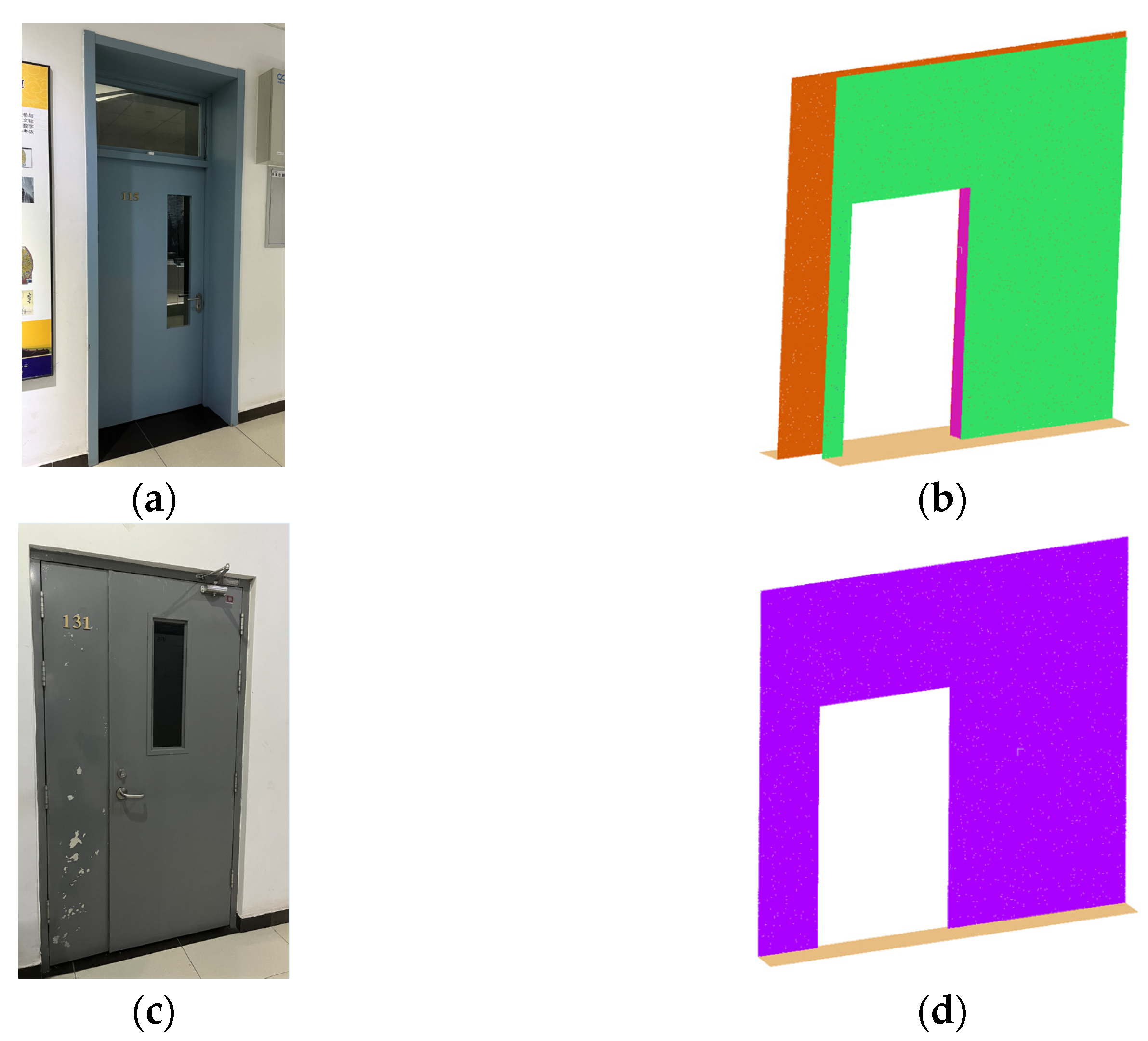
In general, indoor space can be classified in two different applications: management of building components and indoor facilities; and use of indoor spaces [35]. Therefore, indoor space can be defined as a set of structural units with different functions composed of building components. As shown in Figure 1, according to the usage function and indoor navigation requirements, we divide the indoor space into navigable elements such as rooms, corridors and doors. Rooms and corridors are units separated by walls or partitions and enclosed by walls, ceilings and floors. Doors are the units responsible for connecting the various navigation elements in indoor navigation, and can be divided into “thin doors” and “thick doors” according to their characteristics [10,35]. The “thin door” is a two-dimensional plane embedded in an opening in the indoor wall surface. The “thick door” is a three-dimensional space enclosed by a connecting transition space and two “thin doors”, as shown in Figure 2. The connecting transition spaces are located inside the walls between rooms or corridors that have a connecting relationship.
According to the hierarchical relationship between building components and navigation elements, this paper gives the flowchart of information extraction and reconstruction of indoor navigation elements, as shown in Figure 3. Firstly, we extract the building components from the point cloud. Then, the information of indoor navigation elements is produced based on the building components. Finally, the indoor navigation elements and navigation network are reconstructed and represented using the building components. There are four main steps:
  • Building components extraction. Extracting the possible planar data from the point cloud as alternative building components P using the random sample consensus (RANSAC) algorithm [36]. Then the alternative building components are classified and integrated according to their space characteristics to obtain the walls, floors and ceilings;
  • Wall segment restoration. Project the point cloud of the wall surface onto the XOY plane to form the wall segment raster. Then the connectivity of disjoint wall segments is judged according to the relationship between building components. Finally, the energy minimization function is constructed to determine the best connectivity;
  • Navigation element information extraction. Diving building components into navigation elements such as rooms, corridors and connecting transition space based on their geometric features and topological relationships. Then the openings on the wall surface that satisfy the threshold value are extracted as doors. Finally, the navigation elements are optimized according to the relationship between doors and connecting transition space;
  • Navigation element reconstruction and navigation network generation. First, reconstruct the navigation element 3D model using the building components and the extracted navigation element information. Then, the indoor navigation network is generated and represented based on the connectivity and local geometric features between the navigation elements.
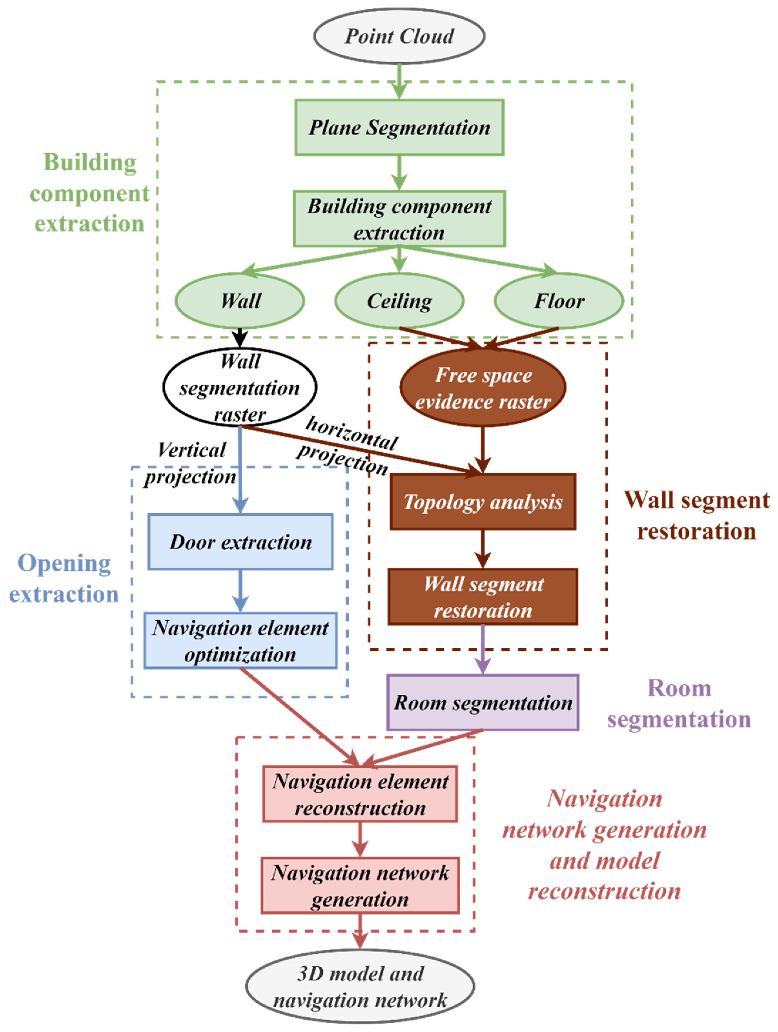
Figure 3. Flowchart for reconstruction of navigation elements and network.
Remotesensing 14 04275 g003

3.2. Building Components Extraction and Wall Segment Restoration

We assume that the wall is perpendicular to the XOY plane. The plane, which is almost perpendicular to the XOY plane and with error less than θ v , is extracted from the alternative building components P as the alternative wall surfaces P wall . Affected by indoor occlusions and pedestrians, alternative wall surfaces include not only occluded wall surfaces, but also occlusions that may be considered as wall surfaces. We deal with occlusions as follows:
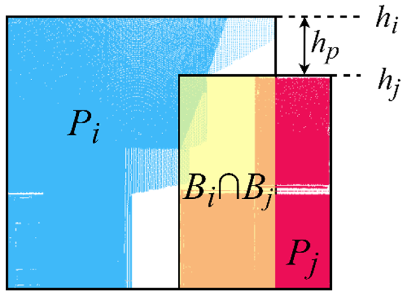
1. Occlusions treatment. First, the wall surfaces satisfying Equation (1) are combined, and then the wall surfaces smaller than the height of the door frame or with an area of less than 1 m2 are excluded [10,37]. However, there may still be some higher occlusions that have not been removed. An optional step can be used to remove higher occlusions. If the height difference between the top of alternative wall surface and the ceiling satisfies Equation (2), the wall surface will be excluded. The point cloud of ceiling and floor can be obtained by the histogram method [38].
P j = { p j | p i , p j P wall : ( a n g ( p i , p j ) < θ b ) ( d i s ( p i , p j ) < d ) ( h i h j > h p ) ( B i B j ) }
where   a n g and d i s represent the angle and the Euclidean distance between the planes. As shown in Figure 4, h i and h j are the height of the top of planes p i and p j , B i and B j are the oriented bounding box of planes p i and p j after projection to the same plane. θ b is the angle threshold, d is the distance threshold, and h p is the height difference threshold between the top of the planes.
P i = { p i | p i P wall : | h c e i l i n g h i | > h p }
where h c e i l i n g represents the height of the ceiling, respectively, and h i represents the height of the alternative wall surface p i ;
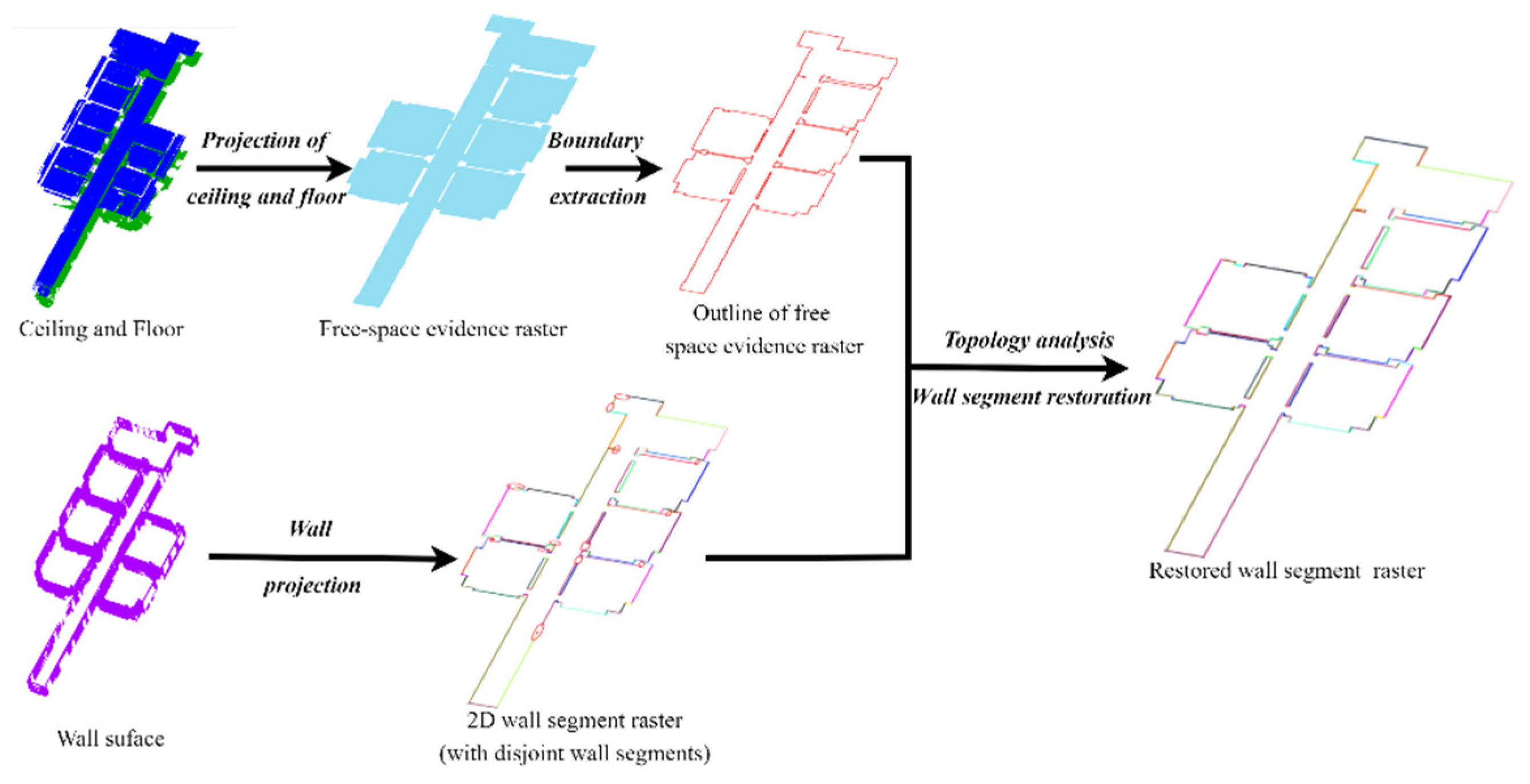
2. Wall segment restoration. The detected wall surface is projected onto the XOY plane using a bottom-up method to generate a 2D wall segment evidence raster. If there are no points in the z-direction within the threshold, then no pixels will be projected on the 2D plane (the threshold is chosen to be the lowest door frame height) [39]. However, not all of the projected wall segments intersect with each other, and these disjoint wall segments should be restored to reconstruct a topologically correct 3D model [40]. The extraction and restoration process of the wall segments is shown in Figure 5.
For the processing flow described in Figure 5, we focus on topology analysis and wall segment restoration. The wall segments can be divided into boundary wall segments and indoor wall segments according to their locations. The boundary wall segments are located at the boundary between the indoor space and the external space. The indoor wall segments are located in the indoor space and are used to cut different structural units. According to the geometric and topological relationships between building elements, it is known that the projection of the outline of free-space evidence raster on the XOY plane coincides with the projection of the boundary wall surfaces, and the adjacent wall surfaces should have the same or adjacent ceilings. Thus, the outlines of the free-space evidence raster are obtained to guide the boundary wall segments for topological analysis. Then, the topological relationships of indoor wall segments are analyzed according to the spatial location of wall segments and ceilings. Algorithm 1 introduces the specific process.
Algorithm 1. Wall segment topology analysis
Input: Wall segment raster: Wall
   Guide line (The outline of a free-space evidence raster): G
   Wall segment search radius: rw
   Connection search radius: rc
   Ceiling: C
Output: Topological relations of wall segment: Tboundary
(1)
W = getDisjointLines (Wall); // Get disjoint wall segments in all wall segments
(2)
for each w W
(3)
  [Pcenter, Pend] = getMidPixelandEndPixel (w);
(4)
e = getForwardDirection (Pcenter, Pend); // Construct the forward direction from Pcenter to Pend
(5)
P = searchClosestPixel (Pend, G, rw); // Search for the nearest pixel in G to Pend within the radius rw
(6)
if (P == )
(7)
Windoor.push_back(w);
(8)
continue;
(9)
end if
(10)
wtarget  
(11)
while ((wtarget == ) && (wtarget != w))
(12)
// Obtain pixels located around P with an angle of less than 90 degrees with e from G
(13)
Ptemp = getForwardPixel(G, e ,   P );
(14)
e = getForwardDirection (P, Ptemp); // Get the forward direction from P to Ptemp
(15)
P Ptemp;
(16)
wtarget = searchWallSegment (P, rw); // Search for wall segments around P within a radius of rw
(17)
end while
(18)
Tboundary.push_back ([w, wtarget]);
(19)
end for
(20)
for each w Windoor
(21)
c = getCeiling (w, C); // Get the ceiling associated with the wall segment
(22)
Pindoor = getEndPixel (w); // Get the endpoint of the wall
(23)
// Get the wall segment that is closest to the Pindoor and has the same or adjacent ceiling as w.
(24)
wtarget = getWallSegments (rc, Pindoor, c, w, Wall);
(25)
Tboundary.push_back ([w, wtarget]);
(26)
end for
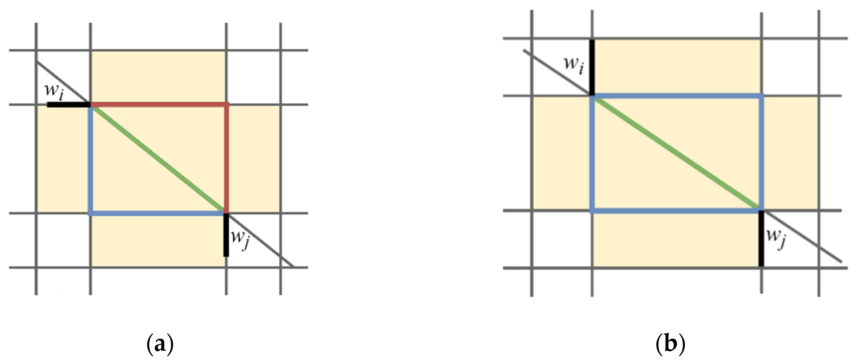
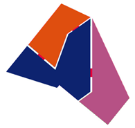
After obtaining the topological relationships between the disjoint wall segments,, we determine whether the wall segments in the Tboundary are parallel to each other based on the angle threshold θ b . For non-parallel wall segments, three potential connection schemes are given, i.e., intersecting, orthogonal and directly connected, as shown in Figure 6a. For parallel wall segments, if the distance between the wall segments is less than the distance threshold d , the wall segments are combined; if the distance between the wall segments is greater than the distance threshold d , two potential connection schemes are given, i.e., orthogonal and directly connected., as shown in Figure 6b.
Figure 6 divides the local XOY plane into different cells by real and potential wall segments. These cells can be given different labels according to their location: indoor “ l i n t ” and outdoor “ l e x t ”. The connection scheme is finally determined by the common edge between the indoor and outdoor cells. The labeling process of the cells can be solved similar to an energy minimization problem [41]. Our minimized energy function consists of data and smoothing terms:
E = λ c V D c ( l c ) + ( 1 λ ) c , c N V c c ( l c , l c )
where c V D c ( l c ) and c , c N V c c ( l c , l c ) represent the data term and the smoothing term. λ represents the balance parameter between the data term and the smoothing term.
The data items are determined by the proportion of each cell that contains free-space evidence raster.
D c ( l c ) = { S V c o c c u p i e d S V c l c l i n t S V c e m p t y S V c l c l e x t
where S V c represents the number of pixels in the cell.   S V c o c c u p i e d represents the number of pixels occupied by the free-space evidence raster in the cell.   S V c e m p t y represents the number of pixels occupied by the empty raster in the cell.
Meanwhile, the smoothing term is determined by the pixel occupancy difference P d i f of the free space-evidence raster between adjacent cells and the weight L(φ) of the common edges of adjacent cells.
V c c ( l c , l c ) = P d i f · L ( φ ) + P d i f P d i f = 1 | S V c o c c u p i e d S V c S V c o c c u p i e d S V c | L ( φ ) = { 0 ,     w c c i n t e r s e c t i n g   c o n n e c t i o n 1 2 ,     w c c d i r e c t   c o n n e c t i o n 1 2 ,     w c c o r t h o g o n a l   c o n n e c t i o n     A N D   ( W i   W j ) 1 ,     w c c o r t h o g o n a l   c o n n e c t i o n     A N D     ( W i   W j )
where S V c and S V c represent the number of pixels in two adjacent cells.   w c c represents the connection relation of common edges of adjacent cells. Generally speaking, the fewer newly added edges in a potential scheme, the more likely it is to become a connected scheme. As shown in Figure 6, the intersection scheme has no new wall segment added. The direct connection scheme adds a new wall segment. The orthogonal scheme adds 1–2 new wall segments. The optimization problem defined in Equation (3) is solved by the method of graph cuts [42]. Then, the wall segments are restored according to the labels of the cells.

3.3. Indoor Room Segmentation

We propose a method that simulates the work of laser scanner to segment indoor space. The specific segmentation process is as follows:
Step 1: The restored wall segment projection raster and the free-space evidence raster are fused;
Step 2: Select a random point within the free-space evidence raster as the laser scanner site location L;
Step 3: Simulate the laser scanner at point L to emit n rays uniformly clockwise and record the wall segments hit by the rays;
Step 4: Extend the wall segment that was hit by the ray to form a plurality of virtual enclosed areas. Then, the enclosed area where L is located is used as the area to be processed in the subsequent steps;
Step 5: The proportion ∂ of real wall segments in the boundary of the virtual enclosed area is calculated according to Equation (6). If the proportion ∂ exceeds the threshold ε , the virtual enclosed area is labeled as the area where the room or corridor is located. Instead, the area is discarded and step 2 is executed;
Step 6: Check whether the virtual enclosed area in step 4 has an adjacency or containing relationship with the already labeled area. If so, the area will be fused with the existing area and labeled as the same area;
Step 7: If the proportion of the labeled area to the free-space evidence raster exceeds α, the segmentation process is complete. The unmarked area is the connecting transition space.
= W r W v W v
where W r represents the real wall and W v represents the boundary of the virtual enclosed area.
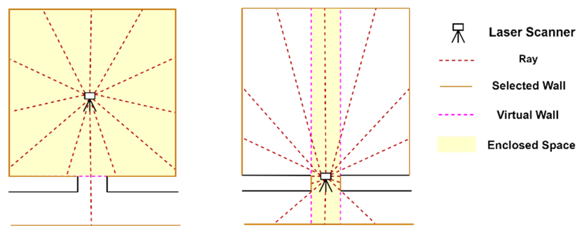
As shown in Figure 7, when scanning within a room, the scanner can usually obtain a larger amount of wall surface data. In this case, it is sufficient to form a virtually enclosed area by adding a small number of wall segment extensions. Whereas, if the scanner is located in a connecting transition space between rooms, it will only obtain less wall surface data to segment room.

3.4. Door Extraction

Most existing methods for extracting indoor doors based on point clouds are projecting the point cloud onto a 2D raster and identifying the openings [2,27,43]. Since the walls are affected by occlusion and the density of the point cloud, different openings projected onto the 2D raster may be identified as the same opening by the connection between pixels. In the projected two-dimensional raster, the openings as doors are usually significantly different in length and width from the other openings caused by occlusion. Thus, we used a method based on statistical graphs of wall projections to fill the missing wall surfaces and extract doors using given thresholds. The method can be divided into four steps:
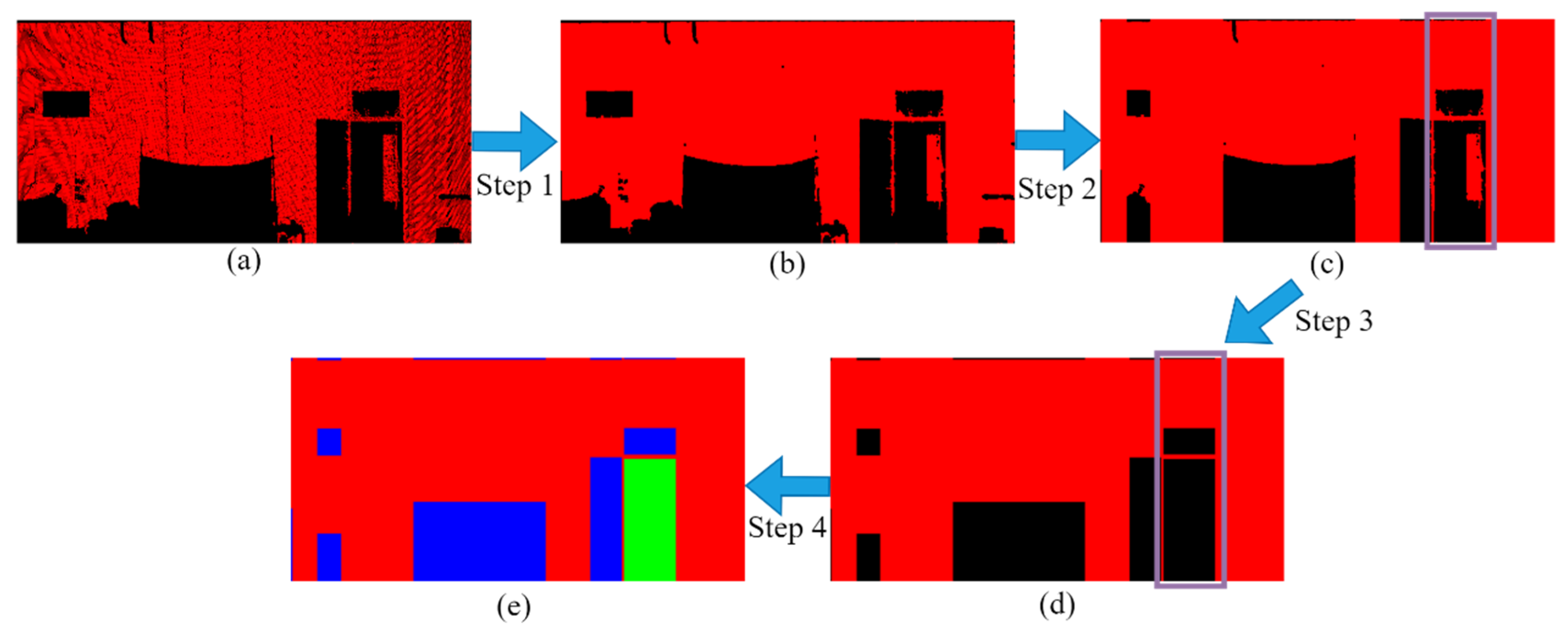
Step 1: The point cloud on the wall surface is projected onto a two-dimensional raster parallel to the wall surface and perpendicular to the XOY plane, as shown in Figure 8a. Then, noise is removed using a morphological open operation, as shown in Figure 8b;
Step 2: The black pixels in each column in Figure 8b are counted and the proportion of black pixels in the columns of the raster is calculated to generate a statistical graph, as shown in Figure 9a. The pixels at the peak of each column are smaller than the threshold P c o l that are filled as wall surface, as shown in Figure 8c;
Step 3: In Figure 8c, columns that have black pixels are continuously above the threshold P c o l and are recognized as local regions in turn. Then, the black pixels in each local region are separately counted by rows and the proportion of black pixels in the rows of the local region is calculated to generate statistical graphs, as shown in Figure 9b. For each local region, the rows above the threshold P r o w are filled as the wall surface and the rows less than the threshold P r o w are filled as black pixels, as shown in Figure 8d;
Step 4: The openings from the processed wall surface that meet the length and width thresholds are selected as doors, as shown in Figure 8e.
Figure 8. Door extraction process. Red represents the wall surfaces. Black represents the openings. Blue represents the alternative results. Green represents the extraction results. (a) is the 2D raster after point cloud projection on the wall surface. (b) is the result of (a) after morphological open operation. (c) is the result after some of the column pixels in (b) are filled. (d) is the result after some of the row pixels in (c) are filled. (e) is the result of the door extraction.
Remotesensing 14 04275 g008
Figure 9. Statistics graph of wall projection raster. (a) represents the column statistics graph in step 2 of Figure 8b represents the row statistics graph of the purple boxed area in Figure 8b. The red line indicates the threshold values. (b) represents the column statistics graph in step 3 of Figure 8c.
Remotesensing 14 04275 g009
After the doors and connection transition spaces are extracted, there are still some “hidden doors” and connection transition spaces that need to be identified. Since some doors are closed during the data collection process, the location of the door may be considered as wall surface in door extraction. Secondly, since point cloud acquired by some laser scanning devices may have local drift. These drifted point clouds will be considered as connecting transition spaces when they appear inside the walls. To solve this problem, the following reasonable rules were made to automatically correct partially undetected doors and incorrectly detected connecting transition spaces. Rule 1 is used to detect “hidden doors”. Rule 2 is used as an optional rule to remove connection transition areas that are incorrectly constructed due to drifting point cloud.
Rule 1: If a “thin door” exists at the location where the connecting transition space connects to a structural unit, another “thin door” also exists at the location where the connecting transition space connects to another structural unit.
Rule 2 (Optional): If there are no “thin doors” on both side of the connecting transition space to the structural unit, the connecting transition space should not exist.

3.5. Navigation Network Generation and Model Reconstruction

After obtaining the information of building components and navigation elements in the indoor space, building components can be integrated based on the hierarchical relationship in Section 3.1 to reconstruct the navigation element models. The reconstructed results can generate not only models with geometric information, but also vector 3D models with semantic information to satisfy the applications of GIS and BIM.
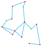
For indoor navigation and route planning, we set the geometric center of the navigation element as a node and the connection relationship obtained from the label information in the connecting transition space or on both sides of the door as an edge to construct the navigation network, as shown in Figure 10a. However, navigation elements connected by only one edge may have a navigation path through the wall [30]. Therefore, some geometric features of indoor spaces need to be incorporated into the construction of navigation networks.
The concavity of the corner point of the navigation element is judged. If the angle of the corner point on the indoor side is ∂ (180° ≤ ∂ < 360°), the corner point is a concave point. When two wall segments on either side of the concave point intersect with the navigation network, these two wall segments are extended to intersect with other wall segments. Then, the local navigation network is reconstructed based on the result of segmentation, as shown in Figure 11. Besides, the structural units connected with more than three other units are set as corridors. As shown in Figure 10b, the navigation network of the corridor is also reconstructed according to the literature [10].

4. Experiments and Results

4.1. Experimental Data and Evaluation Criteria

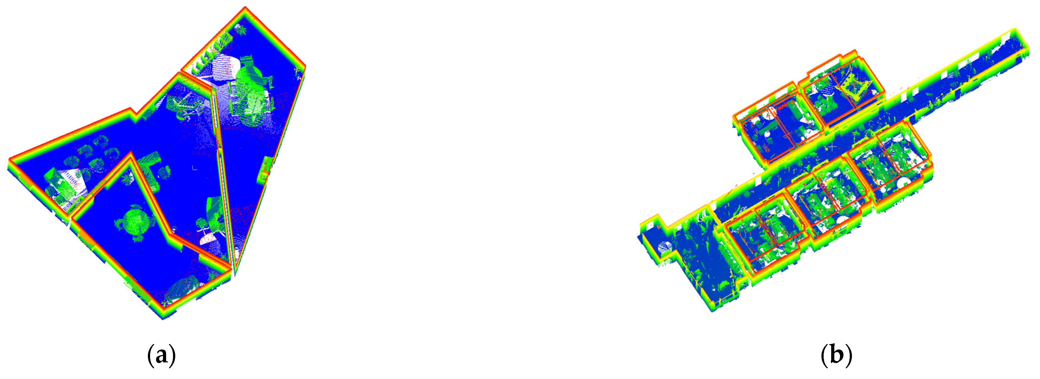
The feasibility of the proposed method was verified by testing seven datasets using C++ and MATLAB on a computer (i7-11700 CPU, 2.5 GHZ and 16 GB RAM), as shown in Figure 12. The Synthetic Point Cloud (Synth) is an indoor environmental simulation data from the datasets of the University of Zurich. Synth includes three irregular rooms and three doors. The real data includes two offices and one room. The first office (Office1) was scanned using a Trimble TX5 terrestrial laser scanner at the Beijing University of Civil Engineering and Architecture. Office1 consists of a long corridor, six rooms and 18 doors. The second office (Office2) is also from the University of Zurich datasets. Office2 consists of a corridor, five rooms and six doors. Another room (Room) is a private residence scanned using a mobile measurement system with a laser scanner (Hokuyo UTM-30LX) [44]. Room consists of six rooms and four doors. In addition, we also selected TUB1, TUB2 second floor and UOM data from the ISPRS Benchmark Dataset. TUB1 data was captured using the Viametris iMS3D system with some missing wall boundaries. TUB1 includes 10 rooms and 23 doors. TUB2 data was captured using a Zeb-Revo sensor with low clutter. The second level of TUB2 includes 10 rooms and 28 doors. UOM data was captured using a Zeb-1 sensor acquired with a moderate level of clutter. UOM includes seven rooms and 14 doors. Three data sets in the Benchmark Dataset contain closed doors.
In order to verify the experimental results, the reconstructed model is evaluated by the following three criteria: completeness; correctness; and accuracy. Completeness is defined as the proportion of reference data in the source data, calculated by Equation (7). Correctness is defined as the proportion of the source data in the reference data, calculated by Equation (8). Accuracy is defined as the geometric proximity of the source data to the reference data and is calculated by Equation (9).
C o m p l e t e n e s s = R e f e r e n c e S o u r c e R e f e r e n c e
C o r r e c t n e s s = R e f e r e n c e S o u r c e S o u r c e
A c c u r a c y = | D i s t a n c e ( V i , S i ) |
where S o u r c e represents the source data, i.e., the door or 2D floor plane of the reconstructed model; R e f e r e n c e represents the reference data, i.e., the door or 2D floor plane of the original point cloud or ground truth model. D i s t a n c e represents the Euclidean distance between data.   V i represents the point on the surface of the reconstructed model. S i represents the closest point to V i on the source data (point cloud/ground truth model).

4.2. Parameter Settings

Table 1 shows the parameters used in this paper for building component extraction and model reconstruction. Four parameters are involved in the building component extraction. θ v is recommended to be 0–5°. θ b , d and h p are used to merge the alternative planes. θ b setting range is recommended to be less than 20°. d setting distance should be less than the minimum thickness of walls. h p is recommended to be greater than the height difference between the top of the highest occlusion and ceiling.
Three parameters are involved in the process of wall segment restoration. r w should be less than the minimum thickness of walls. r c should be greater than one and less than two times of the door width. λ is taken as 0.4–0.6 in our experiments. As shown in the local details in Figure 13, with increasing smoothing terms (i.e., decreasing λ), the local details will be ignored. Similarly, as the data items increase (i.e., λ increases), more details that match the existing data will be revealed. Thus, if the floor and ceiling point cloud is complete, λ should be increased when restoring the wall segment. Similarly, if the ceiling and floor point cloud is missing in localized areas, λ should be decreased. The room segmentation process involves three parameters. n should increase with the complexity of the room layout construction. ε is taken as 0.4–0.8. α should be slightly less than (1-area of connecting transition space /area of indoor space).
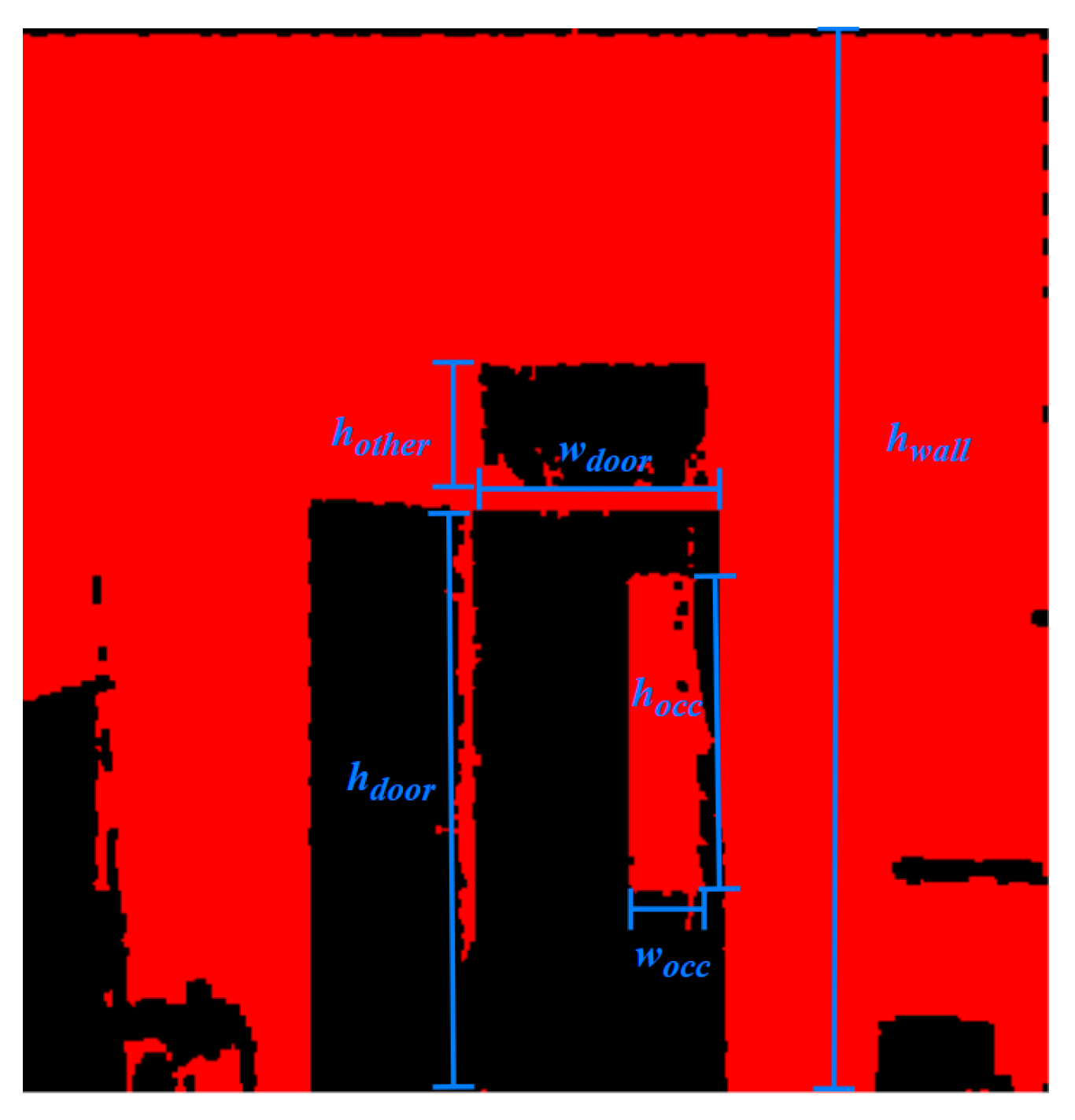
Door extraction process involves six parameters. The door height limit and width limit should be obtained according to the actual situation. P c o l and P r o w can be a unitized scale (e.g., 0.5). The method of determining P c o l is based on the height of the wall where the door is located, the height of the door, the height of the occlusion inside the door and the height of other openings at the location of the door. P c o l can be calculated by Equation (10). Similar to P c o l , the method of determining P r o w is based on the width of the door and the width of the occlusion inside the door. P r o w can be calculated by Equation (11).
P c o l = h d o o r h o c c + h o t h e r h w a l l
P r o w = w d o o r w o c c w d o o r
where h d o o r represents the height of the door, h o c c represents the height of the occlusion, h o t h e r represents the height of other openings at the location of the door, h w a l l represents the height of the wall surface, w d o o r represents the width of the door and w o c c represents the width of the occlusion. As shown in Figure 14.

4.3. Experimental Results

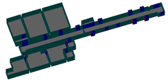
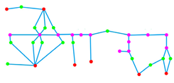
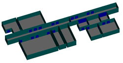
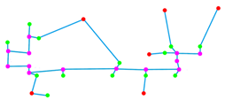
Table 2 shows the reconstructed model and the navigation network, where the model has semantic information not only for the ceiling, floor and walls, but also for the doors and connecting transition space.

5. Discussion

5.1. Model Accuracy Evaluation

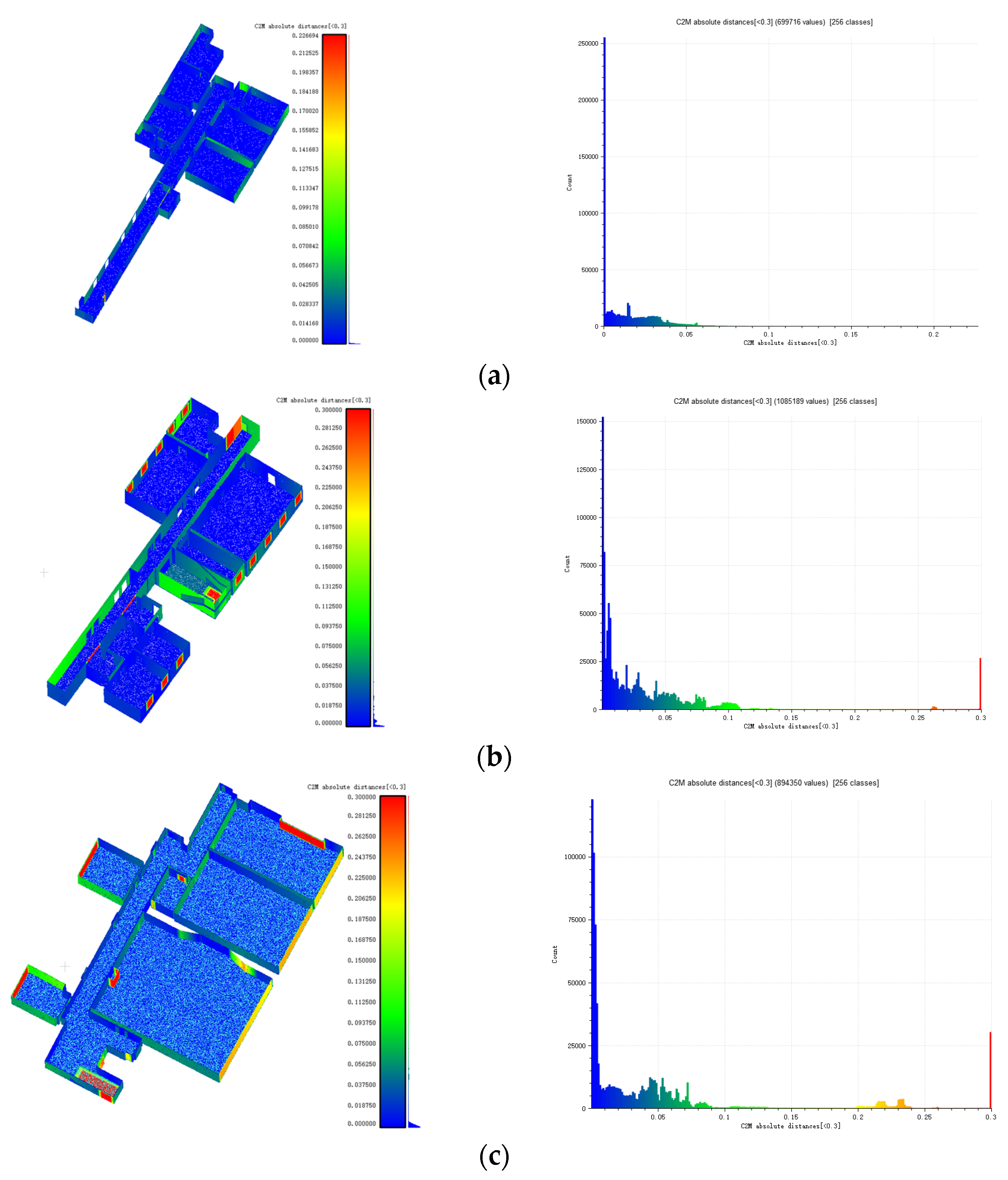
To evaluate the accuracy of the model, the reconstructed results of three data from the ISPRS benchmark dataset were compared with ground truth models. The evaluation used Equation (9) to calculate the unsigned deviation between planes. Figure 15 shows the unsigned distance deviations using colors and plots the statistical histogram. Among them, the deviation in TUB1 data is mainly distributed in the range of 0–5 cm, the mean of distance deviation is about 1.3 cm, the root mean square (RMS) of distance deviation is about 2.2 cm. The deviations in TUB2 data were concentrated in the range of 0–10 cm, the mean of distance deviation was about 3.1 cm, the RMS of distance deviation was about 6.3 cm. The deviation in UOM data is concentrated in the range of 0–9 cm, the mean of distance deviation is about 4.3 cm, the RMS of distance deviation was about 7.3 cm. Compared with other methods submitted to the ISPRS indoor modeling benchmark such as [45], our methods have a higher reconstruction accuracy for TUB1 and TUB2. Meanwhile, the accuracy of the reconstructed models for the UOM dataset is slightly lower.
Since the other four datasets do not have real ground truth models, the unsigned distance deviation between the reconstructed models and the original point cloud is calculated for quantitative evaluation. Figure 16 shows the unsigned distance deviations using colors and plots the statistical histogram. Among them, the deviations in Synth are concentrated between 0–3 cm, the mean of distance deviation is about 2.1 cm, the RMS of distance deviation was about 4.8 cm. The deviations in the data Room are concentrated in the range of 0–10 cm, the mean of distance deviation is about 3.4 cm, the RMS of distance deviation was about 7.2 cm. The deviations in the data Office1 are concentrated in the distribution of 0–10 cm, the mean of distance deviation is about 5.2 cm, the RMS of distance deviation was about 9.7 cm. The deviations in the data Office2 are concentrated in the range of 0–5 cm, the mean of distance deviation is about 3.9 cm, the RMS of distance deviation was about 7.5 cm.

5.2. Room Sgementation Evaluation

We compare the experimental results with the relevant segmentation methods using the same dataset, and the results are shown in Table 3. The method of Ambru [18] et al. assigns different labeling information to each individual segmented region after segmenting the ceiling projection by an extended wall line, however, some regions may be assigned wrong labels due to the local ceiling missing. The morphology-based segmentation method is the more classic segmentation scheme among room segmentation methods, although it cannot clearly delineate the boundaries of rooms. The method proposed by Yang [38] et al. can better divide the indoor space, but for the connecting transition space between rooms, which are directly classified as indoor space or eliminated. Compared with the above three segmentation schemes, the segmentation method in this paper can effectively segment the indoor space and has the following advantages: (i) our room segmentation method can effectively avoid the segmentation error caused by the missing local ceiling; (ii) The segmentation accuracy of each room boundary is ensured; (iii) The connecting transition space between rooms can be well extracted.

5.3. Component Evaluation

As shown in Table 4, by comparing the experimental results of the three datasets provided by the ISPRS benchmark with the terrestrial truth model. The data TUB1 detected 10 rooms with 98.7% correctness and 99.2% completeness of the 2D floor planes. The data TUB2 detected seven rooms with 98.1% correctness and 95.2% completeness of the 2D floor plan. The data UOM detected seven rooms with 98.3% correctness and 93.6% completeness of the 2D floor plan. Table 5 gives the results of the door detection and room connectivity assessment, and the correctness and completeness of the room door detection was greater than 86% in all rooms.
For the remaining four groups of indoor environments without real surface data, the generated models are compared with the point cloud to analyze and evaluate the navigation element extraction results. As shown in Table 6, all four groups of experimental room segmentation results are the same as the correct results, and the correctness and completeness of the results of door detection is greater than 80%.

5.4. Limitations

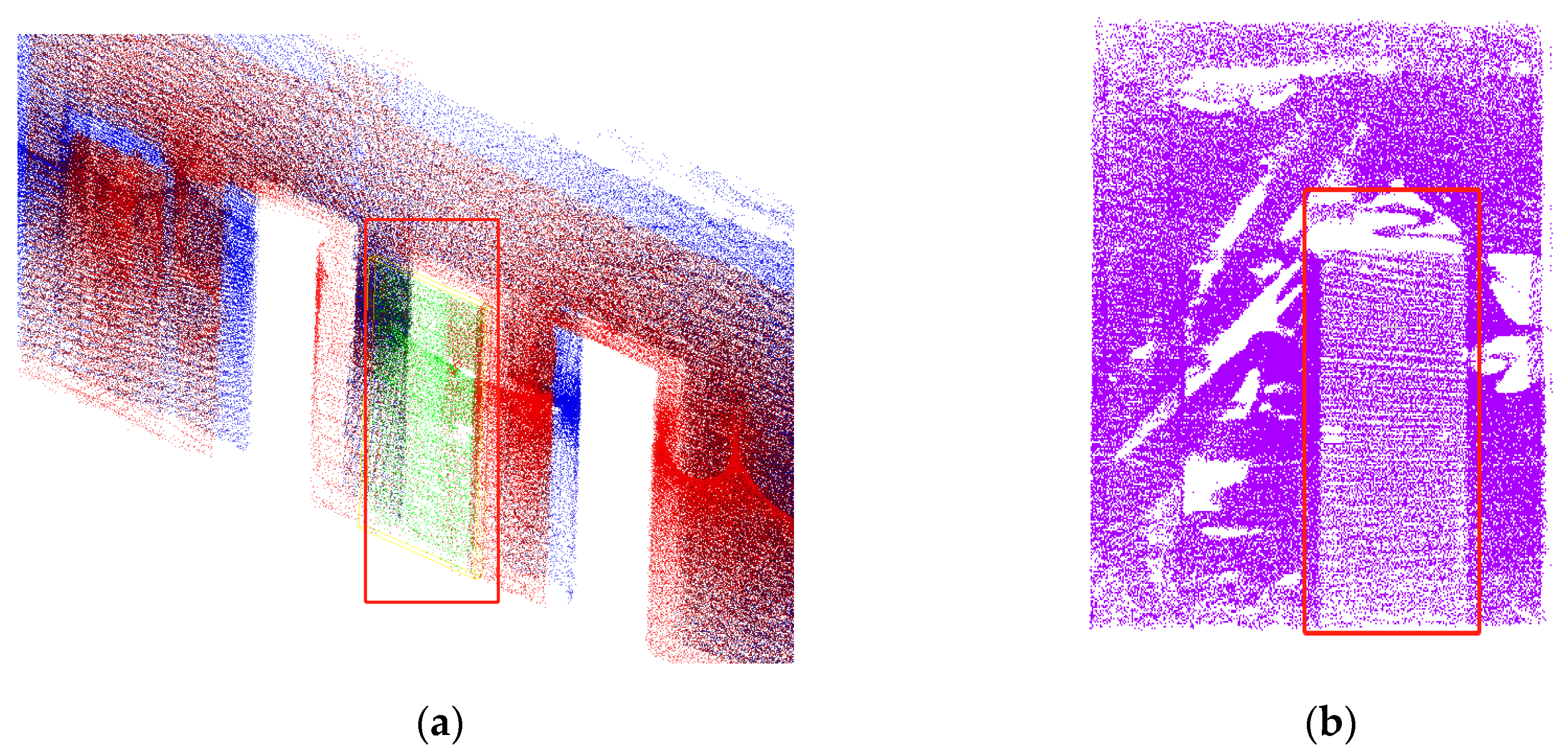
In the above data, most of the information of walls, rooms and doors are detected, but there are some errors in the detection process. In the process of wall restoration, although several given connection schemes are able to restore the missing walls, these schemes are too limited to represent all connection situations due to the complicated building structure. In the door extraction, the “thick doors” with occlusion can be extracted well, but the “thin doors” with a lot of occlusion cannot be extracted in this paper, as shown in Figure 17. Other point cloud information (e.g., density, intensity, color, etc.) can be tried for extraction. Secondly, this paper uses the plane as the building element for navigation element extraction. The reconstruction results will be different from the actual situation when facing building components with larger curvature or rooms with fewer planes. In addition, the laser scanner cannot accurately acquire data on the surface of the object in some scenes due to the influence of the object surface material. Therefore, the method in this paper is also not applicable to indoor scenes where a large number of objects are used that affect the data acquisition by the laser scanner.

6. Conclusions and Future Work

This paper presents methods to automatically reconstruct indoor navigation elements from unstructured 3D point cloud of buildings with occlusions and openings. To reiterate the value of the proposed methods, we summarized the process taking a practical work example as shown in Figure 18. This is a real indoor scene consisting of a long corridor and six rooms. The indoor scene contains a lot of occlusion. We accurately reconstructed the navigation network and the 3D model. This is difficult for other methods to successfully extract some elements such as connecting transition spaces and “hidden doors”. The methods extract possible planes from the point cloud as building components. The walls are restored using the point cloud horizontal projection information. Next, the indoor space is segmented by simulating the work of the laser scanner. Then, we used the statistical graph to fill the missing walls and set thresholds to obtain information about the doors. The reconstructed building models were also optimized using the relationship between doors and connecting transition space. Finally, the indoor navigation element model and the navigation network are generated. The proposed methods were tested on different building datasets with complex structures and occlusions. The experiments show that the method can detect and reconstruct indoor navigation elements and navigation networks without viewpoint information. The mean deviation in the reconstructed model is in the range of 0–5 cm, and the completeness and correctness are greater than 80%. These results demonstrate the robustness and effectiveness of the method. However, the proposed method also has some limitations, for example, for “thin doors” with a large amount of occlusion, the method in this paper is not successful in extracting them and needs to be combined with other point cloud information (e.g., density, intensity, color, etc.). Secondly, the reconstruction results will be different from the actual situation when facing building components with larger curvature or rooms with fewer planes.
In the future, we intend to extend the existing approach to indoor environments containing building structures with large curvature. Facing the missing wall segments caused in cluttered environments, we will try to build a semantic model library to provide better restoration solutions for the missing wall segments. Finally, indoor path planning in cluttered environments is also the next direction we will investigate.

Author Contributions

Conceptualization, G.L., S.W. and S.Z.; methodology, G.L., S.W. and S.Z.; software, G.L. and S.H.; validation, G.L. and S.W.; writing—original draft preparation, G.L.; writing—review and editing, S.W., S.Z. and R.Z.; visualization, G.L. and S.H. All authors have read and agreed to the published version of the manuscript.

Funding

This research is partially supported by National Natural Science Foundation of China (Grant no. 72174031) and the Beijing Key Laboratory of Operation Safety of Gas, Heating and Underground Pipelines.

Institutional Review Board Statement

Not applicable.

Data Availability Statement

The data presented in this study are openly available in [46,47,48].

Acknowledgments

We acknowledge the Visualization and MultiMedia Lab at University of Zurich (UZH) and Claudio Mura for the acquisition of the 3D point clouds, and UZH as well as ETH Zürich for their support to scan the rooms represented in these datasets. The authors acknowledge the ISPRS WG IV/5 for the acquisition of the 3D point clouds.

Conflicts of Interest

There are no conflicts of interest to report.

References

  1. Otero, R.; Lagüela, S.; Garrido, I.; Arias, P. Mobile indoor mapping technologies: A review. Autom. Constr. 2020, 120, 103399. [Google Scholar] [CrossRef]
  2. Xiong, X.; Adan, A.; Akinci, B.; Huber, D. Automatic creation of semantically rich 3D building models from laser scanner data. Autom. Constr. 2013, 31, 325–337. [Google Scholar]
  3. Bi, S.; Yuan, C.; Liu, C.; Cheng, J.; Wang, W.; Cai, Y. A Survey of Low-Cost 3D Laser Scanning Technology. Appl. Sci. 2021, 11, 3938. [Google Scholar] [CrossRef]
  4. Liu, J.; Xu, D.; Hyyppa, J.; Liang, Y. A Survey of Applications With Combined BIM and 3D Laser Scanning in the Life Cycle of Buildings. IEEE J. Sel. Top. Appl. Earth Obs. Remote Sens. 2021, 14, 5627–5637. [Google Scholar] [CrossRef]
  5. Wei, S.; Liu, M.; Zhao, J.; Huang, S. A Survey of Methods for Detecting Indoor Navigation Elements from Point Clouds. Geomat. Inf. Sci. Wuhan Univ. 2018, 43, 2003–2011. [Google Scholar]
  6. Giorgini, M.; Aleotti, J.; Monica, R. Floorplan generation of indoor environments from large-scale terrestrial laser scanner data. IEEE Geosci. Remote Sens. Lett. 2018, 16, 796–800. [Google Scholar]
  7. Ochmann, S.; Vock, R.; Wessel, R.; Klein, R. Automatic reconstruction of parametric building models from indoor point clouds. Comput. Graph. 2016, 54, 94–103. [Google Scholar]
  8. Mura, C.; Mattausch, O.; Villanueva, A.J.; Gobbetti, E.; Pajarola, R. Automatic room detection and reconstruction in cluttered indoor environments with complex room layouts. Comput. Graph. 2014, 44, 20–32. [Google Scholar]
  9. Liu, M.; Wei, S.; Huang, S.; Tang, N. Indoor Navigation Elements Extraction of Room Fineness Using Refining Space Separator Method. Geomat. Inf. Sci. Wuhan Univ. 2021, 46, 221–229. [Google Scholar]
  10. Yang, J.; Kang, Z.; Zeng, L.; Akwensi, P.H.; Sester, M. Semantics-guided reconstruction of indoor navigation elements from 3D colorized points. ISPRS J. Photogramm. Remote Sens. 2021, 173, 238–261. [Google Scholar]
  11. Lehtola, V.V.; Nikoohemat, S.; Nüchter, A. Indoor 3D: Overview on scanning and reconstruction methods. In Handbook of Big Geospatial Data; Springer: Berlin/Heidelberg, Germany, 2021; pp. 55–97. [Google Scholar]
  12. Shaobo, Z.; Zhichen, Y.; Yongsheng, Y.; Chao, S.; Quanyi, H. Study on Evacuation Modeling of Airport Based on Social Force Model. J. Syst. Simul. 2018, 30, 3648. [Google Scholar]
  13. Coughlan, J.M.; Yuille, A.L. Manhattan world: Compass direction from a single image by bayesian inference. In Proceedings of the Seventh IEEE International Conference on Computer Vision, Kerkyra, Greece, 20–27 September 1999; pp. 941–947. [Google Scholar]
  14. Schindler, G.; Dellaert, F. Atlanta world: An expectation maximization framework for simultaneous low-level edge grouping and camera calibration in complex man-made environments. In Proceedings of the 2004 IEEE Computer Society Conference on Computer Vision and Pattern Recognition, CVPR 2004, Washington, DC, USA, 27 June–2 July 2004; p. I-I. [Google Scholar]
  15. CityGML. Available online: https://www.ogc.org/standards/citygml (accessed on 8 July 2022).
  16. Industry Foundation Classes (IFC). Available online: http://technical.buildingsmart.org/standards/ifc/ (accessed on 8 July 2022).
  17. Pintore, G.; Mura, C.; Ganovelli, F.; Fuentes-Perez, L.; Pajarola, R.; Gobbetti, E. State-of-the-art in Automatic 3D Reconstruction of Structured Indoor Environments. In Computer Graphics Forum; John Wiley & Sons, Inc.: Hoboken, NJ, USA, 2020; pp. 667–699. [Google Scholar]
  18. Ambruş, R.; Claici, S.; Wendt, A. Automatic room segmentation from unstructured 3-D data of indoor environments. IEEE Robot. Autom. Lett. 2017, 2, 749–756. [Google Scholar]
  19. Dehbi, Y.; Leonhardt, J.; Oehrlein, J.; Haunert, J.-H. Optimal scan planning with enforced network connectivity for the acquisition of three-dimensional indoor models. ISPRS J. Photogramm. Remote Sens. 2021, 180, 103–116. [Google Scholar]
  20. Yang, F.; Zhou, G.; Su, F.; Zuo, X.; Tang, L.; Liang, Y.; Zhu, H.; Li, L. Automatic indoor reconstruction from point clouds in multi-room environments with curved walls. Sensors 2019, 19, 3798. [Google Scholar]
  21. Nikoohemat, S.; Diakité, A.; Zlatanova, S.; Vosselman, G. Indoor 3D modeling and flexible space subdivision from point clouds. ISPRS Ann. Photogramm. Remote Sens. Spat. Inf. Sci. 2019, 4, 285–292. [Google Scholar]
  22. Bassier, M.; Vergauwen, M. Unsupervised reconstruction of Building Information Modeling wall objects from point cloud data. Autom. Constr. 2020, 120, 103338. [Google Scholar] [CrossRef]
  23. Lim, G.; Oh, Y.; Kim, D.; Jun, C.; Kang, J.; Doh, N. Modeling of architectural components for large-scale indoor spaces from point cloud measurements. IEEE Robot. Autom. Lett. 2020, 5, 3830–3837. [Google Scholar]
  24. Elseicy, A.; Nikoohemat, S.; Peter, M.; Elberink, S.O. Space subdivision of indoor mobile laser scanning data based on the scanner trajectory. Remote Sens. 2018, 10, 1815. [Google Scholar]
  25. Bormann, R.; Jordan, F.; Li, W.; Hampp, J.; Hägele, M. Room segmentation: Survey, implementation, and analysis. In Proceedings of the 2016 IEEE International Conference on Robotics and Automation (ICRA), Stockholm, Sweden, 16–21 May 2016; pp. 1019–1026. [Google Scholar]
  26. Li, L.; Su, F.; Yang, F.; Zhu, H.; Li, D.; Zuo, X.; Li, F.; Liu, Y.; Ying, S. Reconstruction of three-dimensional (3D) indoor interiors with multiple stories via comprehensive segmentation. Remote Sens. 2018, 10, 1281. [Google Scholar]
  27. Michailidis, G.-T.; Pajarola, R. Bayesian graph-cut optimization for wall surfaces reconstruction in indoor environments. Vis. Comput. 2017, 33, 1347–1355. [Google Scholar]
  28. Li, T.; Han, D.; Chen, Y.; Zhang, R.; Zhang, Y.; Hedgpeth, T. IndoorWaze: A Crowdsourcing-Based Context-Aware Indoor Navigation System. IEEE Trans. Wirel. Commun. 2020, 19, 5461–5472. [Google Scholar] [CrossRef]
  29. Zhou, M.; Lin, Y.; Zhao, N.; Jiang, Q.; Yang, X.; Tian, Z. Indoor WLAN Intelligent Target Intrusion Sensing Using Ray-Aided Generative Adversarial Network. IEEE Trans. Emerg. Top. Comput. Intell. 2020, 4, 61–73. [Google Scholar] [CrossRef]
  30. Litao, H.; Lijuan, Z.; Cheng, G.; Aiguo, Z. An indoor navigation network considering walking habits and its generation algorithm. Acta Geod. Cartogr. Sin. 2022, 51, 729. [Google Scholar]
  31. Vasquez-Espinoza, L.; Castillo-Cara, M.; Orozco-Barbosa, L. On the relevance of the metadata used in the semantic segmentation of indoor image spaces. Expert Syst. Appl. 2021, 184, 115486. [Google Scholar]
  32. Pham, T.T.; Reid, I.; Latif, Y.; Gould, S. Hierarchical Higher-Order Regression Forest Fields: An Application to 3D Indoor Scene Labelling. In Proceedings of the 2015 IEEE International Conference on Computer Vision (ICCV), Washington DC, USA, 11–18 December 2015; pp. 2246–2254. [Google Scholar]
  33. Cao, J.; Leng, H.; Lischinski, D.; Cohen-Or, D.; Tu, C.; Li, Y. Shapeconv: Shape-aware convolutional layer for indoor RGB-D semantic segmentation. In Proceedings of the IEEE/CVF International Conference on Computer Vision, Montreal, QC, Canada, 10–17 October 2021; pp. 7088–7097. [Google Scholar]
  34. Menini, D.; Kumar, S.; Oswald, M.R.; Sandström, E.; Sminchisescu, C.; Van Gool, L. A real-time online learning framework for joint 3d reconstruction and semantic segmentation of indoor scenes. IEEE Robot. Autom. Lett. 2021, 7, 1332–1339. [Google Scholar]
  35. Diakité, A.A.; Zlatanova, S.; Alattas, A.F.M.; Li, K.J. Towards Indoorgml 2.0: Updates and Case Study Illustrations. Int. Arch. Photogramm. Remote Sens. Spat. Inf. Sci. 2020, 43, 334–337. [Google Scholar] [CrossRef]
  36. Schnabel, R.; Wahl, R.; Klein, R. Efficient RANSAC for point-cloud shape detection. In Computer Graphics Forum; Blackwell Publishing Ltd.: Oxford, UK, 2007; pp. 214–226. [Google Scholar]
  37. Cui, Y.; Li, Q.; Dong, Z. Structural 3D reconstruction of indoor space for 5G signal simulation with mobile laser scanning point clouds. Remote Sens. 2019, 11, 2262. [Google Scholar] [CrossRef]
  38. Yang, F.; Li, L.; Su, F.; Li, D.; Zhu, H.; Ying, S.; Zuo, X.; Tang, L. Semantic decomposition and recognition of indoor spaces with structural constraints for 3D indoor modelling. Autom. Constr. 2019, 106, 102913. [Google Scholar] [CrossRef]
  39. Wang, R.; Xie, L.; Chen, D. Modeling indoor spaces using decomposition and reconstruction of structural elements. Photogramm. Eng. Remote Sens. 2017, 83, 827–841. [Google Scholar] [CrossRef]
  40. Nikoohemat, S.; Diakité, A.A.; Zlatanova, S.; Vosselman, G. Indoor 3D reconstruction from point clouds for optimal routing in complex buildings to support disaster management. Autom. Constr. 2020, 113, 103109. [Google Scholar]
  41. Previtali, M.; Díaz-Vilariño, L.; Scaioni, M. Indoor Building Reconstruction from Occluded Point Clouds Using Graph-Cut and Ray-Tracing. Appl. Sci. 2018, 8, 1529. [Google Scholar] [CrossRef]
  42. Boykov, Y.; Veksler, O.; Zabih, R. Fast approximate energy minimization via graph cuts. IEEE Trans. Pattern Anal. Mach. Intell. 2001, 23, 1222–1239. [Google Scholar] [CrossRef]
  43. Shi, W.; Ahmed, W.; Li, N.; Fan, W.; Xiang, H.; Wang, M. Semantic Geometric Modelling of Unstructured Indoor Point Cloud. ISPRS Int. J. Geo-Inf. 2018, 8, 9. [Google Scholar] [CrossRef]
  44. Pomerleau, F.; Liu, M.; Colas, F.; Siegwart, R. Challenging data sets for point cloud registration algorithms. Int. J. Robot. Res. 2012, 31, 1705–1711. [Google Scholar] [CrossRef]
  45. Khoshelham, K.; Tran, H.; Acharya, D.; Díaz Vilariño, L.; Kang, Z.; Dalyot, S. The Isprs Benchmark on Indoor Modelling–Preliminary Results. Int. Arch. Photogramm. Remote Sens. Spat. Inf. Sci. 2020, 42, 207–211. [Google Scholar] [CrossRef]
  46. ASL Datasets Repository. Available online: https://projects.asl.ethz.ch/datasets/ (accessed on 8 July 2022).
  47. ISPRS Benchmark on Indoor Modelling. Available online: https://www2.isprs.org/commissions/comm4/wg5/dataset/ (accessed on 8 July 2022).
  48. University of Zurich Dataset. Available online: https://www.ifi.uzh.ch/en/vmml/research/datasets.html (accessed on 8 July 2022).
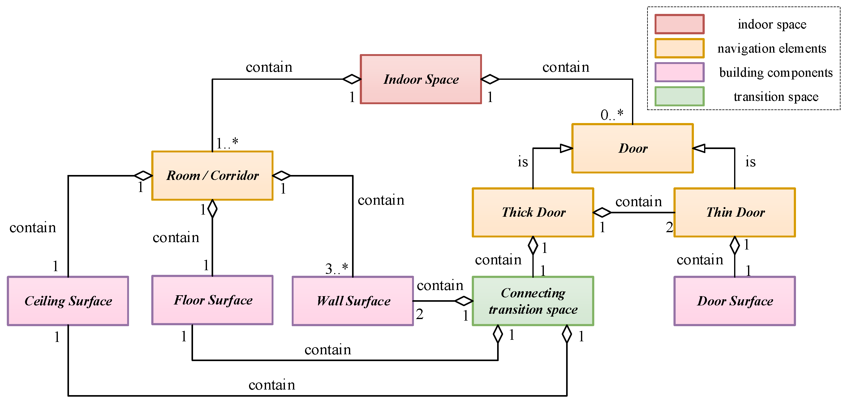
Figure 1. Hierarchy of indoor space navigation elements and building components.
Remotesensing 14 04275 g001
Figure 2. “thick door” and “thin door”: (a) is a photo of “thick door”; (b) is the point cloud of “thick door”; (c) is a photo of “thin door”; and (d) is the point cloud of “thin door”.
Remotesensing 14 04275 g002
Figure 4. Merging alternative wall surfaces. The blue area and the red area are different alternative wall surfaces. The black frame is the oriented bounding box. The translucent yellow area is the intersection area of the oriented bounding boxes.
Remotesensing 14 04275 g004
Figure 5. Wall surface extraction and restoration process.
Remotesensing 14 04275 g005
Figure 6. Potential wall segment connection schemes: (a) non-parallel wall segment connection scheme; (b) parallel wall segment connection scheme. Where W i and W j represent disjoint wall segments with topological relationships. The red lines represent intersecting schemas; the blue lines represent orthogonal schemas; and the green lines represent directly connected schemas. The gray lines represent the division of the free-space evidence raster. Yellow cells will be labeled in next step to finalize connection scheme between W i and W j .
Remotesensing 14 04275 g006
Figure 7. Construct virtual enclosures in different areas.
Remotesensing 14 04275 g007
Figure 10. Corridor navigation network generation and adjustment. The purple dots are corridor nodes. The red dots and green dots are abstract nodes. The thick blue lines indicate the connection relationship between nodes. (a) represents the initial navigation network. (b) represents the corridor node optimized navigation network.
Remotesensing 14 04275 g010
Figure 11. Local navigation network generation and adjustment. The yellow areas indicate the connecting transition space. The burgundy dots are the convex points. The pink dots are the concave points. The red dots and green dots are abstract nodes. The thick blue lines indicate the connection relationship between nodes. The pink lines are the wall segments intersecting with the navigation network.
Remotesensing 14 04275 g011
Figure 12. Datasets: (a) Synth; (b) Office1; (c) Office2; (d) Room; (e) TUB1; (f) TUB2; (g) UOM.
Remotesensing 14 04275 g012aRemotesensing 14 04275 g012b
Figure 13. The effect of the change in λ on wall restoration.
Remotesensing 14 04275 g013
Figure 14. Schematic diagram of the parameters of Equations (10) and (11).
Remotesensing 14 04275 g014
Figure 15. Visualization of unsigned distance deviations on the left and histogram of deviation statistics for the data on the right. (a) represents the accuracy evaluation results of TUB1. (b) represents the accuracy evaluation results of TUB2. (c) represents the accuracy evaluation results of UOM.
Remotesensing 14 04275 g015
Figure 16. Visualization of unsigned distance deviations on the left and histogram of deviation statistics for the data on the right. (a) represents the accuracy evaluation results of Synth. (b) represents the accuracy evaluation results of Room. (c) represents the accuracy evaluation results of Office1. (d) represents the accuracy evaluation results of Office2.
Remotesensing 14 04275 g016
Figure 17. Doors with different geometric features. (a) Thick door (b) Thin door.
Remotesensing 14 04275 g017
Figure 18. Practical work examples. (a) is a real scene. (b) is the real point cloud. (c) is the navigation network. (d) is the 3D semantic model.
Remotesensing 14 04275 g018
Table 1. Summary of parameters for model extraction and reconstruction.
ParameterDescriptionUnits
Building component extraction θ v Angle between alternative building components and alternative wall planeDegree
θ b Angle between alternative wall surfacesDegree
d Distance between alternative wall surfacesMeter
h p Height difference between the top of alternative wall surfacesMeter
Wall
segment
restoration
r w Radius of mutual search of boundary wall segments and guide linesMeter
r c Search radius of connection relations of indoor wall segmentsMeter
λ The balance parameter between the data term and the smoothing term-
Indoor space decomposition n Number of emitted rays-
ε Percentage of real wall segments in the boundary of the virtual enclosed area-
α The percentage of the marked area in the free-space evidence raster-
Door
extraction
h m a x The maximum limit of door heightMeter
h m i n The bottom limit of door heightMeter
w m a x The maximum limit of door widthMeter
w m i n The minimum limit of door widthMeter
P c o l Filling threshold for column pixels on the wall surface-
P r o w Filling threshold for row pixels on the wall surface-
Table 2. Model reconstruction and navigation network generation results.
DataIndoor Space DecompositionNavigation NetworkModel (Hide Ceiling)
Synth Remotesensing 14 04275 i001 Remotesensing 14 04275 i002 Remotesensing 14 04275 i003
Office1 Remotesensing 14 04275 i004 Remotesensing 14 04275 i005 Remotesensing 14 04275 i006
Office2 Remotesensing 14 04275 i007 Remotesensing 14 04275 i008 Remotesensing 14 04275 i009
Room Remotesensing 14 04275 i010 Remotesensing 14 04275 i011 Remotesensing 14 04275 i012
TUB1 Remotesensing 14 04275 i013 Remotesensing 14 04275 i014 Remotesensing 14 04275 i015
TUB2 Remotesensing 14 04275 i016 Remotesensing 14 04275 i017 Remotesensing 14 04275 i018
UOM Remotesensing 14 04275 i019 Remotesensing 14 04275 i020 Remotesensing 14 04275 i021
Table 3. Result comparison of room segmentation methods.
DataTUB1Office1Room
Proposed segmentation method Remotesensing 14 04275 i022 Remotesensing 14 04275 i023 Remotesensing 14 04275 i024
Other segmentation method Remotesensing 14 04275 i025 Remotesensing 14 04275 i026 Remotesensing 14 04275 i027
Ambru, et al.Morphology-based segmentationYang et al.
Table 4. Room reconstruction evaluation results of benchmark dataset.
DataReal Room NumberDetected Real Room NumberCorrectness
on 2D Floor Plane
Completeness
on 2D Floor Plane
TUB110110.9870.992
TUB21090.9810.952
UOM770.9830.936
Table 5. Opening for benchmark data.
DataDoor NumberDetected Door NumberCorrectly Detected Door NumberCorrectness
on Door
Completeness
on Door
TUB12322200.910.87
TUB22829270.930.96
UOM1413120.920.86
Table 6. Experimental results of some experiments without real ground data.
DataReal Room NumberDetected Real Room NumberDetected Wall Surface Number
Synth3325
Office177106
Office26636
Room6629
DataDoor NumberDetected Door NumberCorrectnesson DoorCompletenesson Door
Synth3311
Office118180.880.88
Office25511
Room450.801
Publisher’s Note: MDPI stays neutral with regard to jurisdictional claims in published maps and institutional affiliations.