A Sparse-Model-Driven Network for Efficient and High-Accuracy InSAR Phase Filtering

Abstract

Phase filtering is a vital step for interferometric synthetic aperture radar (InSAR) terrain elevation measurements. Existing phase filtering methods can be divided into two categories: traditional model-based and deep learning (DL)-based. Previous studies have shown that DL-based methods are frequently superior to traditional ones. However, most of the existing DL-based methods are purely data-driven and neglect the filtering model, so that they often need to use a large-scale complex architecture to fit the huge training sets. The issue brings a challenge to improve the accuracy of interferometric phase filtering without sacrificing speed. Therefore, we propose a sparse-model-driven network (SMD-Net) for efficient and high-accuracy InSAR phase filtering by unrolling the sparse regularization (SR) algorithm to solve the filtering model into a network. Unlike the existing DL-based filtering methods, the SMD-Net models the physical process of filtering in the network and contains fewer layers and parameters. It is thus expected to ensure the accuracy of the filtering without sacrificing speed. In addition, unlike the traditional SR algorithm setting the spare transform by handcrafting, a convolutional neural network (CNN) module was established to adaptively learn such a transform, which significantly improved the filtering performance. Extensive experimental results on the simulated and measured data demonstrated that the proposed method outperformed several advanced InSAR phase filtering methods in both accuracy and speed. In addition, to verify the filtering performance of the proposed method under small training samples, the training samples were reduced to 10%. The results show that the performance of the proposed method was comparable on the simulated data and superior on the real data compared with another DL-based method, which demonstrates that our method is not constrained by the requirement of a huge number of training samples.

1. Introduction

Due to the all-weather and all-day characteristics of the synthetic aperture radar (SAR), it plays an important role in remote sensing [1,2,3,4,5]. Simultaneously, the continuous development of SAR has brought more and more development prospects to interferometric SAR (InSAR). At present, InSAR has a wide range of applications such as surface deformation monitoring and terrain mapping [6,7,8,9,10,11]. The basic principle of InSAR measurement technology mainly extracts the phase difference in the primary and secondary images through the observation angle difference of the primary and secondary antennas, and finally inverts the elevation information of the observation area by using the formula between the phase difference and the height.

In the whole InSAR processing flow, noise is inevitably added to the InSAR phase, which can be divided into three categories: system noise, coherent noise, and noise introduced by signal processing [12,13]. The presence of noise severely destroys the follow-up phase unwrapping step, which reduces the accuracy of phase unwrapping and even obtains the incorrect results [14,15]. Therefore, interferometric phase filtering is a necessary processing step and has also become a very important technology in InSAR measurement.

Since the invention of InSAR technology, a large number of effective interferometric phase filtering approaches have been developed, and the traditional methods fall into four main categories (i.e., spatial domain local filters [16,17,18,19,20], spatial domain nonlocal (NL) filters [21], transform domain local filters [22,23,24,25,26], and transform domain NL filters [27,28]). The main idea of spatial domain local filters is to filter out the phase noise in the space domain using a local window with pixels. A well-known spatial domain local filter is the Lee filter [18]. Unlike spatial domain filters, the transform domain local filters denoise the interferogram in the transform domain such as the Goldstein filter [26]. However, the above two kinds of filters cannot balance the noise suppression ability and phase detail preservation ability well. In order to further enhance the phase detail preservation capability while ensuring effective noise suppression, the spatial and transform domain NL filters have been proposed, which utilize the patch-by-patch method to measure the patch similarity of the interferogram and the weighted average to restore the interferometric phase [14] such as NL-InSAR [21] and InSAR-BM3D [28]. Although NL filters can consider both noise suppression and phase detail preservation, they suffer from a huge computational cost due to abundant similar block operations. Aiming to bridge this regret, a series of newly advanced filtering algorithms have been proposed [29,30,31,32,33,34].

Over the past few years, deep learning (DL) has been successfully applied to interferogram denoising due to the powerful feature extraction and calculation ability of convolutional neural networks (CNNs) such as Phi-Net [31] and PFNet [30]. However, there are two key problems with the vast majority of existing CNNs. On one hand, the underlying structure of the purely data-driven CNN with a black-box nature is difficult to interpret, that is, it lacks interpretability. Of course, interpretability is an important feature in many fields because it relates to conceptual understanding and the development of knowledge frontiers [35]. On the other hand, most modern CNNs need to learn a large number of parameters, so they excessively depend on huge amounts of data. In other words, a vast majority of CNNs improve the accuracy at the cost of increasing the network complexity. However, in many fields such as in [36,37], the performance of the network trained with small training sets will be significantly reduced, and even inferior to the traditional methods.

In recent years, a promising technique that unrolls the SR algorithm into network architectures was developed by Gregor et al. [38]. Compared to modern CNNs, the unrolled network not only has a sufficient theoretical basis, but also contains fewer layers and parameters, which do not rely on huge training sets. Therefore, some novel networks based on the idea of unrolling the SR algorithm into CNN have been proposed such as in [39,40]. However, since SR algorithm unrolling has not been applied to InSAR phase denoising, we attempted to combine this technique into this field. Inspired by [39,40,41,42], we designed an InSAR phase filtering model and established a model-driven CNN to filter the noisy interferograms.

In this article, we propose a sparse-model-driven network (SMD-Net) for efficient and high-accuracy InSAR phase filtering. In the method, we first establish a SR model for interferometric phase filtering. Then, the SMD-Net is designed as an iteration-based CNN architecture by unrolling each iteration process of the iterative shrinkage-thresholding algorithm (ISTA) [43] to solve the phase filtering model into a block. In each block, a CNN module with a local block and global context (GC) [44] block is established to adaptively learn the sparse domain transform of each iteration in ISTA. Finally, due to dealing with complex-valued data, our method is carried out by exploiting the idea of separating the real and imaginary parts of the interferometric phase. In short, the SMD-Net models the interferometric phase filtering process, rather than relying entirely on data fitting as most networks do and its network structure is simple. It thus improves the filtering performance and computational efficiency at the same time. The experimental results on the simulated and measured data demonstrate that the proposed method outperformed the Lee filter [18], Goldstein filter [26], InSAR-BM3D filter [28], ISTA-based filtering method, and the PFNet [30] in both precision and speed. Furthermore, the filtering performance of the SMD-Net on 10% of the original training samples was also slightly better than that of the PFNet. The main contributions of our work are as follows.

(1)

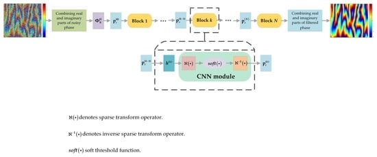
We first built an InSAR phase filtering model. Then, the SMD-Net was designed based on the idea of unrolling the ISTA algorithm of solving the model into a simple network architecture, which enhanced the interpretability of the network. Subsequently, the SMD-Net transformed the interferometric phase into a real matrix consisting of the real and imaginary parts of the phase to achieve a complex-valued filtering operation.

(2)

Unlike the traditional ISTA algorithm setting the sparse transform by handcrafting, the SMD-Net exploits a CNN module to automatically learn the sparse basis operation, which enhances the filtering performance.

(3)

Plenty of simulated and measured experiments illustrate that the proposed method achieves efficiency and high-precision filtering.

The rest of this article is organized as follows. Section 2 describes the InSAR phase noise principle and the InSAR phase SR filtering model. We introduce the design of the SMD-Net and loss function in Section 3. In Section 4, we describe a method of generating the training and testing data, experimental details, and experimental metrics. Extensive experiments on the simulated and real data are conducted in Section 5. Section 6 further discusses the performance of the proposed method under small training samples. Section 7 presents our conclusions.

2. Principle and Model

In what follows, we provide a brief review of the formulation of the interferometric phase and focus on designing the interferometric phase filtering model by analyzing the formulation. This work is to prepare for the subsequent unrolling of the InSAR phase filtering algorithm.

2.1. InSAR Phase Noise Principle

The interferogram $\mathsf{\Gamma }$ is defined as the conjugate product of a pair of single-look complex SAR images.

$$\mathsf{\Gamma }=z_1·z_2^{*}=\left|z_1·z_2^{*}\right|e^{j(\mathsf{\phi })}$$

(1)

where $z_1$ and $z_2$ are the two complex SAR images; * indicates the complex conjugate; and $\mathsf{\phi }$ denotes the measured interferometric phase with noise. The phase noising model with additive noise is as follows.

$$\mathsf{\phi }={\mathsf{\phi }}_c+n_{\mathsf{\gamma }}$$

(2)

where ${\mathsf{\phi }}_c$ denotes the clear interferometric phase and n_γ is the zero-mean additive Gaussian noise associated with the coherence coefficient γ, which is expressed as:

$$\gamma =\frac{E\left(z_1·z_2^{*}\right)}{\sqrt{E\left({\left|z_1\right|}^2\right)·E\left({\left|z_2\right|}^2\right)}}$$

(3)

The interferometric phase noise level is correlated with the coherence coefficient γ. The higher the coherence coefficient, the lower the noise level.

It is worth noting that the value range of the interferometric phase is distributed in (−π, π]. Hence, phase denoising is implemented in the complex field in for the subsequent phase unwrapping steps. Employing a mathematical manipulation on Equation (2), we obtain the following expression.

$$p=e^{j\mathsf{\phi }}=e^{j({\mathsf{\phi }}_c+n_{\gamma })}={\mathsf{\phi }}_r+j{\mathsf{\phi }}_i$$

(4)

where p indicates the interferogram and ${\mathsf{\phi }}_r$ and ${\mathsf{\phi }}_i$ denote the real and imaginary parts of p, respectively. According to the analysis of [45], ${\mathsf{\phi }}_r$ and ${\mathsf{\phi }}_i$ can be given by.

$$\begin{array}{l}{\mathsf{\phi }}_r=\cos ({\mathsf{\phi }}_c+n_{\gamma })=N_c\cos \left({\mathsf{\phi }}_c\right)+n_{{\gamma }_c}\\ {\mathsf{\phi }}_i=\sin ({\mathsf{\phi }}_c+n_{\gamma })=N_c\sin \left({\mathsf{\phi }}_c\right)+n_{{\gamma }_s}\end{array}$$

(5)

where $n_{{\gamma }_c}$ and $n_{{\gamma }_s}$ are defined as the zero-mean additive noise, and N_c is a phase quality evaluation metric related to the coherent coefficient γ. Finally, combining Equations (4) and (5), the formulation of the interferometric phase is derived as follows.

$$p=N_c·p_c^{}+n$$

(6)

where $n=n_{{\gamma }_c}+j{n}_{{\gamma }_s}$ denotes the noise of the interferogram and $p_c^{}=e^{j{\mathsf{\phi }}_c}$ is the ideal interferogram.

2.2. InSAR Phase SR Filtering Model

The conventional SR model for recovering a single from a measurement is as follows.

$$y=\mathsf{\Phi }x+n$$

(7)

where $y\in {ℝ}^M$ is the measurement; $\mathsf{\Phi }\in {ℝ}^{M\times N}$ is dubbed the measurement matrix; $x\in {ℝ}^N$ is the recovered signal; and $n\in {ℝ}^M$ is the noise.

According to Section 2.1, the InSAR phase filtering model can be modeled as.

$$p=\mathsf{\Phi }{p}_c^{}+n$$

(8)

Aiming to solve Equation (8), it is transformed into the following convex optimization problem.

$${\widehat{p}}_c=\underset{p_c}{\arg \min }\frac{1}{2}{‖\mathsf{\Phi }{p}_c-p‖}_2^2+\lambda {‖\mathsf{\psi }{p}_c‖}_1$$

(9)

where $\mathsf{\psi }{p}_c$ is a sparse representation of $p_c$; ψ denotes a certain transform such as Wavelet, Fourier and so on; and λ is a tunable soft threshold parameter.

The main iterative steps of solving Equation (9) by the ISTA algorithm are as follows.

$$h^{\left(k\right)}=p_c{}^{\left(k-1\right)}-\alpha {\mathsf{\Phi }}^H\left(\mathsf{\Phi }{p}_c{}^{\left(k-1\right)}-p\right)$$

(10)

$$p_c{}^{\left(k\right)}={\mathsf{\psi }}^H\mathrm{soft}\left(\mathsf{\psi }{h}^{\left(k\right)},\lambda \right)={\mathsf{\psi }}^H\mathrm{sign}(\mathsf{\psi }{h}^{\left(k\right)})\max \left\{\left|\mathsf{\psi }{h}^{\left(k\right)}\right|-\lambda ,0\right\}$$

(11)

where α indicates the step size; sign(⋅) denotes a sign function; Φ^H is the conjugate transpose of Φ; and $h^{\left(k\right)}$ is the residual error in iteration k. However, the sparse transform ψ and parameters such as α and λ are hand-crafted, which results in the algorithm being nonadaptive. Moreover, ISTA usually suffers from a huge calculative burden due to its large number of iterative steps.

We chose the identity matrix as the measurement matrix Φ by the formulation of the interferometric phase. It can be seen from the above analysis that the phase filtering is operated in the complex domain to achieve high-precision phase unwrapping. Therefore, taking advantage of the idea of separating real and imaginary parts, the noisy phase p, the ideal phase $p_c^{}$, and the measurement matrix Φ are transformed as

$$p_R=\left(\begin{array}{l}{\mathsf{\phi }}_r\\ {\mathsf{\phi }}_i\end{array}\right),p_{c_R}^{}=\left(\begin{array}{l}{\mathsf{\phi }}_{cr}\\ {\mathsf{\phi }}_{ci}\end{array}\right)$$

(12)

$${\mathsf{\Phi }}_R=\left(\begin{array}{cc}{\mathsf{\Phi }}_r& -{\mathsf{\Phi }}_i\\ {\mathsf{\Phi }}_i& {\mathsf{\Phi }}_r\end{array}\right)$$

(13)

where ${\mathsf{\phi }}_{cr}$ and ${\mathsf{\phi }}_{ci}$ are the real and imaginary parts of the ideal interferogram $p_c$, and ${\mathsf{\Phi }}_r$ and ${\mathsf{\Phi }}_i$ denote the real and imaginary parts of the measurement matrix Φ, respectively.

In the end, the filtered interferometric phase is obtained by the real part ${\mathsf{\phi }}_r^{\prime }$ and imaginary part ${\mathsf{\phi }}_i^{\prime }$ of the recovered interferometric phase as follows.

$${\mathsf{\phi }}^{\prime }=\angle \left({\mathsf{\phi }}_r^{\prime }+j{\mathsf{\phi }}_i^{\prime }\right)$$

(14)

3. Methodology

According to the phase filtering model established in Section 2.2, which aimed at performing a fast yet accurate filtering method, we propose a sparse-model-driven network (SMD-Net) for efficient and high-accuracy InSAR phase filtering by combining the interpretability and fewer parameters of SR and the speed advantage of the CNN. Inspired by the idea of the unrolled SR algorithms, the designed network casts the phase filtering model into the unrolled network and implements the complex operation of the unrolled network. In the filtering process shown in Figure 1, first of all, the SMD-Net is trained by employing the real and imaginary parts of the training datasets obtained by Equation (12). Then, the real and imaginary parts of the noisy interferograms (testing data) are entered into the trained SMD-Net, and the filtered real and imaginary parts corresponding to the input are recombined into the estimated interferometric phase using Equation (14). Finally, the filtered phase patches are spliced together by using an image fusion algorithm. Next, we will introduce this section in detail from the design of the SMD-Net and the loss function.

3.1. Network Architecture

3.1.1. The SMD-Net Architecture

Nowadays, some phase filtering methods [29,30,31] based on DL have achieved a better filtering performance than conventional filtering approaches. Nevertheless, they are purely data-driven, which means that these networks rely on a huge data volume and their underlying structures are difficult to interpret. In addition, these networks generally consist of many layers and learn a large number of parameters, which lead to great increases in the computational burden of the network. Considering that SR algorithms model the physical processes underlying the problem and a few parameters, we designed the SMD-Net by employing the idea of unrolling the ISTA algorithm. Unlike the existing based-DL phase filtering methods, the SMD-Net focuses on the interferometric phase filtering model rather than relying entirely on the data fitting and its network structure is simple. It thus is expected to improve the filtering performance and computational efficiency at the same time. The architecture of the SMD-Net is shown in Figure 2.

In the SMD-Net, each network block is equivalent to an iterative process in the traditional ISTA algorithm. To improve the filtering performance and computational efficiency, we exploited a CNN module that automatically learns the sparse transform instead of the artificial sparse transform in the traditional ISTA algorithm. The CNN module is shown in Figure 3.

From each block in Figure 2, ℵ(·) and ${\aleph }^{-1}$(·) functions in the CNN module replace the sparse basis ψ and the conjugate transpose of ψ in the traditional ISTA, respectively. Thus, Equation (9) is transformed as

$${\widehat{p}}_c=\underset{p_c}{\arg \min }\frac{1}{2}{‖\mathsf{\Phi }{p}_c-p‖}_2^2+\lambda {‖\aleph \left(p_c\right)‖}_1$$

(15)

The iterative process in ISTA converts to each block operation in the SMD-Net. Now, we can take the kth block as an example for detailed analysis.

Step 1: The SMD-Net transfers the model parameters of block k − 1 corresponding to the ISTA algorithm parameters to block k by making use of back-propagation. Then, $h^{\left(k\right)}$ is updated by

$$h^{\left(k\right)}=p_c{}^{\left(k-1\right)}-\alpha {\mathsf{\Phi }}^H\left(\mathsf{\Phi }{p}_c{}^{\left(k-1\right)}-p\right)$$

(16)

where α indicates the step size; Φ^H is the conjugate transpose of Φ; and $h^{\left(k\right)}$ is the residual error in the kth block.

Step 2: In order to satisfy the second term of Equation (15), (i.e., the sparse constraint). In the first stage of the CNN module, $h^{\left(k\right)}$ is sparsely represented as $\aleph \left(h^{\left(k\right)}\right)$ ℵ(·) is a function that automatically learns the sparse domain.

Step 3: The CNN module takes $\aleph \left(h^{\left(k\right)}\right)$ and λ as inputs. The kth filtered result in the sparse domain is calculated by

$$s^{\left(k\right)}=\mathrm{soft}\left(\aleph \left(h^{\left(k\right)}\right),\lambda \right)=\mathrm{sign}(\aleph \left(h^{\left(k\right)}\right))\max \left\{\left|\aleph \left(h^{\left(k\right)}\right)\right|-\lambda ,0\right\}$$

(17)

Step 4: The ${\aleph }^{-1}$(·) function is designed on the constraint of ${\aleph }^{-1}\left(·\right)\times \aleph \left(·\right)=\mathrm{I}$ to obtain the kth filtered result in the spatial domain. The result is obtained by

$$p_c{}^{\left(k\right)}={\aleph }^{-1}\left(s^{\left(k\right)}\right)$$

(18)

where $\mathsf{\psi }{p}_c$ is a sparse representation of $p_c$; ψ denotes a certain transform such as Wavelet, Fourier and so on; and λ is a tunable soft threshold parameter.

The SMD-Net is a combination of the merits of modern CNN and the ISTA algorithm. On one hand, the CNN can quickly process the operations between network layers, which makes up for the disadvantage of traditional ISTA algorithms relying on a large number of iterations, thus improving the computational efficiency. On the other hand, interpretability and a few parameters with specific meanings of the ISTA algorithm overcome the drawback that the CNN learns abundant parameters using a large amount of training data and improves the accuracy and the stability of the method.

3.1.2. CNN Module Architecture

To achieve the most suitable sparse representation of $h^{\left(k\right)}$ and enhance the performance of the SMD-Net, we exploited a CNN module to automatically learn the sparse transform instead of the traditional hand-crafted presets one. The CNN module is shown in Figure 3, and it contains the sparse transform ℵ(·), soft(·) function, and inverse transform ${\aleph }^{-1}$(·). The front end of ℵ(⋅) is a local feature extraction module. In order to combine the global phase information, a GC block [44] is connected to the back end of ℵ(·) to extract the global feature of the phase. ℵ(·) can be represented by the following expression.

$$\aleph \left(h^{\left(k\right)}\right)=GC\left(\delta \times {\mathsf{\Gamma }}_1{h}^{\left(k\right)}+\left(1-\delta \right)\times {\mathsf{\Gamma }}_2\mathrm{ReLU}\left({\mathsf{\Gamma }}_1{h}^{\left(k\right)}\right)\right)$$

(19)

where Γ₁ represents a convolution operator with M_f filters of the size M_s × M_s; Γ₂ is another convolution operator corresponding to M_f filters of the size M_s × M_s × M_f; δ denotes the weight; ReLU (x) = max (0, x); and GC(·) represents a GC block.

Moreover, the inverse transform function ${\aleph }^{-1}$(·) is the mirror-symmetrical architecture of ℵ(·). The constraint ${\aleph }^{-1}\left(·\right)\times \aleph \left(·\right)=\mathrm{I}$ is required to obtain the filtered phase in the spatial domain. The two convolution operations in ${\aleph }^{-1}$(·) are the same as in ℵ(·), but the order is switched.

In the kth block of the SMD-Net, Equation (15) can be written as

$$p_c{}^{\left(k\right)}=\underset{p_c}{\arg \min }\frac{1}{2}{‖p_c-h^{\left(k\right)}‖}_2^2+\lambda {‖\aleph \left(p_c\right)‖}_1$$

(20)

Finally, according to ℵ(·) and ${\aleph }^{-1}$(·), Equation (15) can be expressed in the following form.

$$p_c{}^{\left(k\right)}={\aleph }^{-1}\left(\mathrm{soft}\left(\aleph \left(h^{\left(k\right)}\right),\lambda \right)\right)$$

(21)

The CNN module is exploited to automatically learn the appropriate sparse basis and parameters, which not only bridges the regret of the hand-crafted setting in the conventional ISTA, but also enhances the performance of the SMD-Net for InSAR phase filtering.

3.2. Loss Function

The SMD-Net is trained with the training data ${\left\{p_i,p_{ci}\right\}}_{i=1}^{N_{tr}}$, in which $p_i$ and $p_{ci}$ are the measurement and the labels, respectively, and N_tr is the number of the training samples. Then, the loss function is defined as:

$$loss=\frac{{\rho }_1}{N_{tr}}{{\displaystyle {\sum }_{i=1}^{N_{tr}}‖{\widehat{p}}_{c_i}-p_{c_i}‖}}_2^2+\frac{{\rho }_2}{N\times N_{tr}}{{\displaystyle {\sum }_{k=1}^N{\displaystyle {\sum }_{i=1}^{N_{tr}}‖{\aleph }^{-1}\left(\aleph \left(h_i^{\left(k\right)}\right)\right)-h_i^{\left(k\right)}‖}}}_2^2$$

(22)

where N denotes the total number of the SMD-Net block; ${\rho }_1$ and ${\rho }_2$ indicate the weight parameters of the two constraint items; ${\widehat{p}}_{c_i}$ and $p_{c_i}$ are the ith interferogram estimated; h^(k) the ith ideal interferogram; and $h_i^{\left(k\right)}$ represents the residual error in the kth SMD-Net block.

4. Experiments

4.1. Experimental Data

It is well-known that training a deep network requires at least a few hundred or more training datasets with labels. Of course, training the SMD-Net also needs enough interferograms with noise corresponding to the ideal interferograms. In order to obtain a large number of labeled training sets, we generated abundant noisy interferograms with corresponding ideal interferograms by utilizing a digital elevation model (DEM). This is helpful in enhancing the phase detail characteristic similarity between the simulated and measured interferograms [46,47]. The simulated interferometric phase can be obtained as follows:

$${\mathsf{\phi }}_c=\arg \left(e^{j2\pi \left(H/h_a\right)}\right)$$

(23)

where H is the height value of the DEM; arg(·) represents the complex argument operator; and h_a indicates the ambiguity height, which was set to 92.13 m and was consistent with the measured InSAR data used in subsequent experiments.

According to the formulation of the interferometric phase in Section 2.1, the level of noise is related to the coherence coefficient γ, and the higher the coherence value, the less the noise in the InSAR phase data. Hence, interferograms with different coherence coefficients were simulated in order to enhance the generalization ability of the network. The coherence coefficients were in the range of [0.5, 0.95] and the interval was 0.05, which is helpful in that the network adapts to the noise level of a large number of real interferograms.

The generation manner of the simulated training sets is as follows. A simulated clean interferogram, shown in Figure 4b, is generated by employing the DEM (as illustrated in Figure 4a) of the eastern part of Turkey with the size of 2048 × 2048 from the SRTM 1Sec HGT based on Equation (23). Ten noise interferograms were generated by adding different levels of noise whose coherence coefficients were [0.5, 0.95] to the clean interferograms. Noisy interferograms with coherence coefficients of 0.5 and 0.95 are shown in Figure 4c,d. In this paper, we divided the whole interferogram into interferogram patches with the size 256 × 256 with a 0.5 overlap rate to obtain enough training sets and improve the computational efficiency. Among them, each noise interferogram with a coherence coefficient was cropped into a group containing 225 patches. Hence, the total number of interferogram patches with 2250 patches contained ten groups.

Figure 5a shows the DEM with the size of 1024 × 1024 from SRTM 1Sec HGT, which was used to generate the testing data illustrated in Figure 5b. Ten noise interferograms with different coherence coefficients were obtained by adding noise in the same way as the training data, among which the coherence coefficients of 0.5 and 0.95 are shown in Figure 5c,d. These testing interferograms with the different noise levels were also cut into 490 patches like the training data.

4.2. Experimental Details

In this article, we analyzed the performance of the SMD-Net on the experimental results of the simulated and measured data. The proposed method outperformed the previous three widely-used methods (i.e., the Lee filter [18], Goldstein filter [26], and InSAR-BM3D filter [28]) and the two methods based on DL (Phi-Net [31] and PFNet [30]). For a fair comparison, all experiments were carried out on an Inter^® Core™ i7-2790K CPU with 4 Gb random access memory (RAM) and an NVIDIA GeForce GTX 980 Ti GPU, where the previous three widely-used methods were performed in MATLAB R2016b and the proposed method was tested in Pytorch.

Inspired by the work of [39], the SMD-Net contained nine blocks (i.e., nine iterations), each of which had the same network structure as follows: Γ₁ is a convolution operator with 32 filters of the size 3 × 3; Γ₂ is another convolution operator corresponding to 32 filters of the size 3 × 3 × 32. In our experiments, the SMD-Net was trained with the first 2000 interferograms of the training sets obtained in Section 4.1 by utilizing the Adam optimization [48] with a batch size of two. We set the initial learning rate, λ, α, and δ as 0.0001, 0.01, 0.2, and 0.1, respectively.

4.3. Evaluation Metrics

The objective of phase filtering is to suppress noise and preserve interferometric phase details as much as possible. Therefore, the precision of a filtering approach is evaluated by considering both the denoising ability and the phase detail preservation ability. Moreover, the computational complexity is also an important problem for phase filtering, so the evaluation of computational efficiency is essential. In order to compare the performance of filtering methods more intuitively, we adopted two evaluation methods based on the image and data, namely, qualitative evaluation and quantitative evaluation. Qualitative evaluation is implemented directly by the naked eye, which is highly subjective and the evaluation results are not entirely desirable. In contrast, quantitative evaluation has a certain theoretical basis, so the evaluation results are highly reliable. In this paper, the mean-square error (MSE) [49] representing the difference between the filtered interferometric phase and the corresponding ground truth, the number of residues (NOR) [50] used to reflect the denoising ability of a filtering method, the mean structural similarity index (MSSIM) [51] reflecting the phase detail feature preservation ability of a filtering method, and running time (T) were adopted to assess the experiments on the simulated data. In view of lacking the ground truth of the real InSAR data, the no-reference metric Q [52] is a quantitative assessment index of balancing between phase detail preservation and denoising, and the higher this is, the more powerful the phase detail preservation capacity.

5. Results

5.1. Results on the Simulation Data

After obtaining the trained network, in the testing stage, a noisy interferogram with a coherence coefficient of 0.5 shown in Figure 6b from the simulated testing sets was used to qualitatively assess the performance of the proposed method in this article. Figure 6a is the corresponding reference interferogram. In order to validate the proposed method, we compared it with the Lee filter [18], Goldstein filter [26], InSAR-BM3D filter [28], traditional ISTA algorithm [43], Phi-Net [31], and PFNet [30]. All filtered results are illustrated in Figure 7. Figure 7(a1–g1) represents the filtered interferograms of the seven approaches, respectively. Qualitative evaluation with the naked eye showed that the result of the proposed method was closest to the ideal interferogram shown in Figure 6a. We calculated the difference phases of the seven filtered results and the corresponding ideal interferogram, respectively, and show the difference images in Figure 7(a2–g2). From Figure 7(a2–g2), we can see that the difference image of the proposed method was closest to zero, which further verified that the filtered result obtained by the proposed method was most similar to the ideal interferogram. Moreover, the SSIM maps shown in Figure 7(a3–g3) were computed to assess the capability of the phase detail preservation, where it can be seen that the SSIM map of the proposed method (Figure 7(g3)) had the most regions whose values were close to 1 amongst all of the testing methods. The above preliminary comprehensive qualitative analysis showed that the proposed method had the best visual performance in both the suppression noise and phase edge detail preservation.

The qualitative evaluation is too subjective and unstable, and testing only a noisy interferogram is haphazard. Therefore, we calculated the mean MSE and MSSIM of all results obtained by the experiments on all of the testing sets with the same coherence coefficients, and these results are shown in Figure 8. In Figure 8, we can intuitively see that the MSE of the proposed method was lower and the MSSIM was higher than the six reference methods. This demonstrates that the proposed method has the characteristics of the best noise suppression and phase detail feature preservation capabilities among the seven methods.

Finally, the mean values of all metrics are presented in

Table 1. The metrics of the seven methods on the simulated interferogram. MSSIM is the core accuracy index. T is the speed index.

Methods	MSE (Rad2)	NOR	MSSIM	T (s)
Lee [18]	1.62	293.48	0.36	4.39
Goldstein [26]	1.24	91.12	0.50	5.41
InSAR-BM3D [28]	0.63	0	0.74	6.97
ISTA [43]	1.13	185.34	0.51	9.73
Phi-Net [31]	0.66	0	0.74	0.86
PFNet [30]	0.54	0	0.79	0.76
SMD-Net (Ours)	0.50	0	0.81	0.11

. In Table 1, the proposed method had the highest MSSIM, lowest MSE, and NOR among the seven methods. Through a comprehensive comparison, the performance of the proposed method was optimal among the seven methods. In detail, the NORs of the proposed method, InSAR-BM3D, Phi-Net, and PFNet were equal to 0, which demonstrates that the denoising ability of the four methods is powerful. However, the proposed method could better balance between the noise reduction and phase edge feature preservation because it had the highest MSSIM and the lowest MSE. Furthermore, the running time (T) of the proposed method was the shortest. Compared to Phi-Net and PFNet, the mean T of the proposed method was 87.2% and 85.5% faster, respectively. This means that the proposed method had the most powerful computational capability among the seven methods.

5.2. Results on the Real Data

In order to validate the performance of the proposed method in real data, we employed two measured interferograms with the size of 512 × 512 pixels to perform the test experiments. As shown in Figure 9, these were provided by the Sentinel-1 SAR satellite. In order to prove the filtering performance of the proposed method in different shapes and different coherence areas, Figure 9a,b shows a high-coherence area A with a dense fringe and low-coherence area B with flatness, respectively.

The seven methods were used in area A, as shown in Figure 9a and the results are shown in Figure 10a–g, respectively. From the perspective of vision, the proposed method has a more powerful noise reduction capacity than the Lee filter, Goldstein filter, InSAR-BM3D filter, and traditional ISTA. Compared to Phi-Net and PFNet, their denoising abilities were comparable, but it can be seen from the black rectangles in Figure 10e–g that the phase detail feature preservation ability of the proposed method was stronger.

Next, we computed the number of residues (NOR), the no-reference metric Q, and the running time (T), listed in

Table 2. The metrics of the seven methods on the measured interferogram of area A. Metric Q is the core accuracy index. T is the speed index.

Methods	NOR	Metric Q	T (s)
Lee [18]	2506	30.86	16.70
Goldstein [26]	1404	48.73	22.00
InSAR-BM3D [28]	66	71.38	31.26
ISTA [43]	12	54.21	81.67
Phi-Net [31]	2	82.30	11.90
PFNet [30]	0	83.87	2.97
SMD-Net (Ours)	6	90.43	1.43

, to assess the performance of the proposed method more accurately. From Table 2, it can be seen that the NOR of the proposed method was lower than that of the Lee filter, Goldstein filter, InSAR-BM3D filter, and ISTA algorithm, and its metric Q was higher than that of the four methods. This strongly proves that our method was superior to the four reference methods in both the noise suppression and preservation of edge detail. Furthermore, compared with the Phi-Net and PFNet, the NOR of the proposed method was higher, but its metric Q was 9.9% and 7.8% higher, respectively, which demonstrates that the proposed method was superior to the Phi-Net and PFNet in the phase edge detail preservation (i.e., it provided a well-balanced noise reduction and fringe detail preservation). From the perspective of processing efficiency, the running time of the proposed method was the shortest with only 1.43 s among the seven methods and was 51.9% faster than the PFNet. In conclusion, the proposed method performed better than the six reference approaches in both the filtering performance and speed.

Area A is a high-coherence area with dense fringe. Therefore, in order to prove the adaptability of the proposed method to different terrain regions with different levels of noise, we selected a flat area (area B shown in Figure 9b) of low coherence to experiment further. The filtering results of the seven methods are shown in Figure 11a–g. From Figure 11a–g, we can see that our method offers the best-balanced noise suppression and the preservation of the phase edge texture. In more detail, the denoising ability of the proposed method was obviously stronger than the three widely-used methods. The traditional ISTA algorithm lacks a denoising ability, but also suffers from a serious loss of phase details. As shown in the black rectangles in Figure 11e–g, compared with the Phi-Net and PFNet, it was obvious that the proposed method preserved the phase detail features more completely, while the PFNet filtering excessively resulted in a serious loss of phase details. Similarly, the indicators of all of the results obtained by the seven methods were calculated for a quantitative assessment and are listed in

Table 3. The metrics of the seven methods on the measured interferogram of area B. Metric Q is the core accuracy index. T is the speed index.

Methods	NOR	Metric Q	T (s)
Lee [18]	5980	25.67	18.36
Goldstein [26]	4430	44.55	22.97
InSAR-BM3D [28]	444	65.82	29.45
ISTA [43]	203	41.08	82.85
Phi-Net [31]	70	63.96	6.79
PFNet [30]	10	74.10	2.87
SMD-Net (Ours)	81	88.76	1.77

. The performance of the proposed method was obviously better than that of the three widely-used methods, the ISTA algorithm and Phi-Net. Then, the proposed method has a 19.8% higher metric Q compared with PFNet. Combined with the quantitative indexes of area A and area B as shown in Table 2 and Table 3, we can see that the performance reduction in the PFNet was significantly higher than that of the proposed method. This proves that the proposed method had better generalization.

6. Discussion

In order to further analyze the performance of the SMD-Net under the small training samples, in the 10 groups of interferogram patches in Section 4.1, 200 interferogram patches were selected starting from the first interferogram patch in each group at an interval of 10 interferograms as new training sets. Then, the SMD-Net was retrained with the training sets. The indicators of the testing results on the simulated data are listed in

Table 4. The metrics of the PFNet trained with 2250 samples and the SMD-Net trained with 200 samples on the simulated data. MSSIM is the core accuracy index. T is the speed index.

Method	Samples	MSE (Rad2)	NOR	MSSIM	T (s)
PFNet [30]	2250	0.54	0	0.79	0.76
SMD-Net (Ours)	200	0.59	0	0.79	0.11

. As can be seen in Table 4, the MSE of the proposed method was 9.3% higher, but the MSSIM of the proposed method was equal to that of PFNet and its T was 85.5% faster. Therefore, it can be seen that the performance of the SMD-Net trained with 200 training samples was comparable to the PFNet trained with 2250 training samples. Unlike the PFNet, the performance of the SMD-Net was not constrained by the requirement of the data volume.

Like the simulated data, we processed the measured data utilizing the SMD-Net trained with 200 training samples to analyze the filtering performance of the proposed method. The filtering result of area A (Figure 9a) is shown in Figure 12b, and we can see intuitively from the black rectangles in Figure 12a,b that the phase detail features of the result obtained by our method were better preserved. Next, a flat and low-coherence area B (Figure 9b) was processed to prove the generalization of the proposed method. The black rectangles in Figure 12c,d also showed that the proposed method had a stronger phase edge texture preservation capability.

Furthermore, the quantitative indicators of the two areas were calculated and are listed in

Table 5. The metrics of the PFNet trained with 2250 samples and the SMD-Net trained with 200 samples on area A. Metric Q is the core accuracy index. T is the speed index.

Methods	Samples	NOR	Metric Q	T (s)
PFNet [30]	2250	0	83.87	2.97
SMD-Net (Ours)	200	14	88.60	1.52

and

Table 6. The metrics of the PFNet trained with 2250 samples and the SMD-Net trained with 200 samples on area B. Metric Q is the core accuracy index. T is the speed index.

Methods	Samples	NOR	Metric Q	T (s)
PFNet [30]	2250	10	74.10	2.87
SMD-Net (Ours)	200	126	86.78	1.45

. Table 5 and Table 6, compared with the PFNet, it could be observed that the NORs of the proposed method were higher in both areas, but their metric Qs were higher. This indicates that the PFNet caused the serious loss of phase fringe detail information due to over filtering and its phase detail feature preservation capability was inferior to the proposed method. In addition, we could calculate that the metric Qs of the results obtained by processing area A and area B with the proposed method were 5.6% and 17.1% higher than that of the PFNet, respectively. To sum up, it can be seen that the filtering performance of the SMD-NET trained with 200 training samples outperformed that of the PFNet trained with 2250 training samples.

7. Conclusions

In this article, we propose a sparse-model-driven network (SMD-Net) for efficient and high-accuracy InSAR phase filtering. The SMD-Net was designed by casting the mathematical derivation steps of the traditional ISTA algorithm into the network structure. Unlike the ISTA algorithm, in each block of the SMD-Net, a CNN module was established to adaptively learn the sparse transform instead of the hand-crafted setting. The SMD-Net not only significantly reduced the network complexity, but was also combined with the merit of automatically learning the parameters and sparse transform of CNN. It can thus improve the filtering performance and speed at the same time. Finally, plenty of experiments were performed to validate the proposed method.

We assessed the proposed method qualitatively and quantitatively on the simulated and measured InSAR data. The experimental results on the simulated and measured data demonstrated that the proposed method could better balance the abilities of the noise suppression and phase fringe texture preservation than the several reference filtering methods. In addition, the speed of the proposed method was very fast. Compared with the PFNet, the SMD-Net was 85.5% and 51.9% faster on the simulated and measured data, respectively. Aiming to validate the performance of the proposed method was not limited by the requirement of the number of training samples, so the experiments were carried out again when the number of training samples was decreased to 10%. Compared with the PFNet trained with 2250 samples, the performance of the proposed method was comparable on the simulated data. In the experiments on the real data, the Qs of the results obtained by processing high-coherence and low-coherence areas with the proposed method were 5.6% and 17.1% higher, respectively. This proves that the comprehensive performance of our method outperformed that of the six competitive approaches, even with small samples.

References

1. Zhang, T.; Zhang, X. A Full-Level Context Squeeze-and-Excitation ROI Extractor for SAR Ship Instance Segmentation. IEEE Geosci. Remote Sens. Lett. 2022, 19, 4506705. [Google Scholar] [CrossRef]
2. Fischer, G.; Papathanassiou, K.P.; Hajnsek, I. Modeling and Compensation of the Penetration Bias in InSAR DEMs of Ice Sheets at Different Frequencies. IEEE J. Sel. Top. Appl. Earth Obs. Remote Sens. 2020, 13, 2698–2707. [Google Scholar] [CrossRef]
3. Zhang, T.; Zhang, X. HTC+ for SAR Ship Instance Segmentation. Remote Sens. 2022, 14, 2395. [Google Scholar] [CrossRef]
4. Xu, X.; Zhang, X.; Zhang, T. Lite-YOLOv5: A Lightweight Deep Learning Detector for On-Board Ship Detection in Large-Scene Sentinel-1 SAR Images. Remote Sens. 2022, 14, 1018. [Google Scholar] [CrossRef]
5. Zhang, T.; Zhang, X.; Ke, X.; Liu, C.; Xu, X.; Zhan, X.; Wang, C.; Ahmad, I.; Zhou, Y.; Pan, D.; et al. HOG-ShipCLSNet: A Novel Deep Learning Network with HOG Feature Fusion for SAR Ship Classification. IEEE Trans. Geosci. Remote. Sens. 2021, 60, 5210322. [Google Scholar] [CrossRef]
6. Wang, H.; Zhou, Y.; Fu, H.; Zhu, J.; Yu, Y.; Li, R.; Zhang, S.; Qu, Z.; Hu, S. Parameterized Modeling and Calibration for Orbital Error in TanDEM-X Bistatic SAR Interferometry over Complex Terrain Areas. Remote Sens. 2021, 13, 5124. [Google Scholar] [CrossRef]
7. Zhu, X.X.; Wang, Y.; Montazeri, S.; Ge, N. A Review of Ten-Year Advances of Multi-Baseline SAR Interferometry Using TerraSAR-X Data. Remote Sens. 2018, 10, 1374. [Google Scholar] [CrossRef] [Green Version]
8. Wang, H.; Fu, H.; Zhu, J.; Liu, Z.; Zhang, B.; Wang, C.; Li, Z.; Hu, J.; Yu, Y. Estimation of subcanopy topography based on single-baseline TanDEM-X InSAR data. J. Geod. 2021, 95, 84. [Google Scholar] [CrossRef]
9. Hu, J.; Ge, Q.; Liu, J.; Yang, W.; Du, Z.; He, L. Constructing Adaptive Deformation Models for Estimating DEM Error in SBAS-InSAR Based on Hypothesis Testing. Remote Sens. 2021, 13, 2006. [Google Scholar] [CrossRef]
10. Richter, N.; Froger, J.L. The role of Interferometric Synthetic Aperture Radar in detecting, mapping, monitoring, and modelling the volcanic activity of Piton de la Fournaise, La Réunion: A review. Remote Sens. 2020, 12, 1019. [Google Scholar] [CrossRef] [Green Version]
11. Moreira, J.; Schwabisch, M.; Fornaro, G.; Lanari, R.; Bamler, R.; Just, D.; Steinbrecher, U.; Breit, H.; Eineder, M.; Franceschetti, G.; et al. X-SAR Interferometry: First Results. IEEE Trans. Geosci. Remote Sens. 1995, 33, 950–956. [Google Scholar] [CrossRef]
12. Xu, G.; Gao, Y.; Li, J.; Xing, M. InSAR phase denoising: A review of current technologies and future directions. IEEE Geosci. Remote Sens. Mag. 2020, 8, 64–82. [Google Scholar] [CrossRef] [Green Version]
13. Zebker, H.A.; Villasenor, J. Decorrelation in interferometric radar echoes. IEEE Trans. Geosci. Remote Sens. 1992, 30, 950–959. [Google Scholar] [CrossRef] [Green Version]
14. Xia, X.G.; Wang, G.Y. Phase Unwrapping and A Robust Chinese Remainder Theorem. IEEE Signal Process. Lett. 2007, 14, 247–250. [Google Scholar] [CrossRef]
15. Suksmono, A.B.; Hirose, A. Interferometric SAR image restoration using Monte Carlo metropolis method. IEEE Trans. Signal Process. 2002, 50, 290–298. [Google Scholar] [CrossRef]
16. Wang, Q.S.; Huang, H.F.; Yu, A.X.; Dong, Z. An Efficient and Adaptive Approach for Noise Filtering of SAR Interferometric Phase Images. IEEE Geosci. Remote Sens. Lett. 2011, 8, 1140–1144. [Google Scholar] [CrossRef]
17. Abdallah, W.B.; Abdelfattah, R. A modification to the ASM filter for improving SAR interferograms. In Proceedings of the 21st European Signal Processing Conference (EUSIPCO 2013), Marrakech, Morocco, 9–13 September 2013; pp. 1–5. [Google Scholar]
18. Lee, J.S.; Papathanassiou, K.P.; Ainsworth, T.L.; Grunes, M.R.; Reigber, A. A new technique for noise filtering of SAR interferometric phase images. IEEE Trans. Geosci. Remote Sens. 1998, 36, 1456–1465. [Google Scholar]
19. Chao, C.F.; Chen, K.S.; Lee, J.S. Refined filtering of interferometric phase from InSAR data. IEEE Trans. Geosci. Remote Sens. 2013, 51, 5315–5323. [Google Scholar] [CrossRef]
20. Fu, S.H.; Long, X.J.; Yang, X.; Yu, Q.F. Directionally adaptive filter for synthetic aperture radar interferometric phase images. IEEE Trans. Geosci. Remote Sens. 2013, 51, 552–559. [Google Scholar] [CrossRef]
21. Deledalle, C.A.; Denis, L.; Tupin, F. NL-InSAR: Nonlocal interferogram estimation. IEEE Trans. Geosci. Remote Sens. 2011, 4, 1441–1452. [Google Scholar] [CrossRef]
22. Quereda, A.M.; Lopez-Sanchez, J.M.; Selva, J.; Gonzalez, P.J. An improved phase filter for differential SAR interferometry based on an iterative method. IEEE Trans. Geosci. Remote Sens. 2018, 56, 4477–4491. [Google Scholar] [CrossRef] [Green Version]
23. Zha, X.J.; Fu, R.S.; Dai, Z.Y.; Liu, B. Noise reduction in interferograms using the wavelet packet transform and wiener filtering. IEEE Geosci. Remote Sens. Lett. 2008, 5, 404–408. [Google Scholar]
24. Bian, Y.; Mercer, B. Interferometric SAR phase filtering in the wavelet domain using simultaneous detection and estimation. IEEE Geosci. Remote Sens. 2011, 4, 1396–1416. [Google Scholar] [CrossRef]
25. Baran, I.; Stewart, M.; Kampes, B.; Lilly, P. A modification to the Goldstein radar interferogram filter. IEEE Geosci. Remote Sens. 2011, 4, 1396–1416. [Google Scholar] [CrossRef] [Green Version]
26. Goldstein, R.M.; Werner, C.L. Radar interferogram filtering for geophysical applications. Geophys. Res. Lett. 1998, 25, 4035–4038. [Google Scholar] [CrossRef] [Green Version]
27. Xu, H.; Li, Z.; Li, S.; Liu, W.; Li, J.; Liu, A.; Li, W. A Nonlocal Noise Reduction Method Based on Fringe Frequency Compensation for SAR Interferogram. IEEE J. Sel. Top. Appl. Earth Obs. Remote Sens. 2021, 14, 9756–9767. [Google Scholar] [CrossRef]
28. Sica, F.; Cozzolino, D.; Zhu, X.X.; Verdoliva, L.; Poggi, G. INSAR-BM3D: A nonlocal filter for SAR interferometric phase restoration. IEEE Trans. Geosci. Remote Sens. 2018, 56, 3456–3467. [Google Scholar] [CrossRef] [Green Version]
29. Sun, X.; Zimmer, A.; Mukherjee, S.; Kottayil, N.K.; Ghuman, P.; Cheng, I. DeepInSAR—A Deep Learning Framework for SAR Interferometric Phase Restoration and Coherence Estimation. Remote Sens. 2020, 12, 2340. [Google Scholar] [CrossRef]
30. Pu, L.; Zhang, X.; Zhou, Z.; Shi, J.; Wei, S.; Zhou, Y. A Phase Filtering Method with Scale Recurrent Networks for InSAR. Remote Sens. 2020, 12, 3453. [Google Scholar] [CrossRef]
31. Sica, F.; Gobbi, G.; Rizzoli, P.; Bruzzone, L. Φ-Net: Deep Residual Learning for InSAR Parameters Estimation. IEEE Trans. Geosci. Remote Sens. 2021, 59, 3917–3941. [Google Scholar] [CrossRef]
32. Kang, J.; Hong, D.; Liu, J.; Baier, G.; Yokoya, N.; Demir, B. Learning Convolutional Sparse Coding on Complex Domain for Interferometric Phase Restoration. IEEE Tran. Neural Netw. Learn. Syst. 2021, 32, 826–840. [Google Scholar] [CrossRef] [PubMed] [Green Version]
33. Ojha, C.; Fusco, A.; Pintp, I.M. Interferometric SAR phase denoising using proximity-based K-SVD technique. Sensors 2019, 19, 2684. [Google Scholar] [CrossRef] [PubMed] [Green Version]
34. Luo, X.; Wang, X.; Wang, Y.; Zhu, S. Efficient InSAR Phase Noise Reduction via Compressive Sensing in the Complex Domain. IEEE J. Sel. Top. Appl. Earth Obs. Remote Sens. 2018, 11, 1615–1632. [Google Scholar] [CrossRef]
35. Monga, V.; Li, Y.L.; Eldar, Y.C. Algorithm Unrolling: Interpretable, Efficient Deep Learning for Signal and Image Processing. IEEE Signal Process. Mag. 2021, 38, 18–44. [Google Scholar] [CrossRef]
36. Ronneberger, O.; Fischer, P.; Brox, T. U-Net: Convolutional Networks for Biomedical Image Segmentation. In Proceedings of the Medical Image Computing and Computer-Assisted Intervention, Munich, Germany, 5–9 October 2015; Navab, N., Hornegger, J., Wells, W.M., Frangi, A.F., Eds.; Springer International Publishing: Cham, Switzerland, 2015; pp. 234–241. [Google Scholar]
37. Ibtehaz, N.; Rahman, M.S. MultiResUNet: Rethinking the U-Net Architecture for Multimodal Biomedical Image Segmentation. Neural Netw. 2019, 121, 74–87. [Google Scholar] [CrossRef] [PubMed]
38. Gregor, K.; LeCun, Y. Learning Fast Approximations of Sparse Coding. In Proceedings of the 27th International Conference on International Conference on Machine Learning, Madison, WI, USA, 21–24 June 2010. [Google Scholar]
39. Zhang, J.; Ghanem, B. ISTA-Net: Interpretable Optimization-Inspired Deep Network for Image Compressive Sensing. In Proceedings of the 2018 IEEE/CVF Conference on Computer Vision and Pattern Recognition, Salt Lake City, UT, USA, 18–23 June 2018; pp. 1828–1837. [Google Scholar]
40. Jin, K.H.; McCann, M.T.; Froustey, E.; Unser, M. Deep Convolutional Neural Network for Inverse Problems in Imaging. IEEE Trans. Image Process. 2017, 26, 4509–4522. [Google Scholar] [CrossRef] [PubMed] [Green Version]
41. Chen, Y.; Pock, T. Trainable Nonlinear Reaction Diffusion: A Flexible Framework for Fast and Effective Image Restoration. IEEE Trans. Pattern Anal. Mach. Intell. 2017, 39, 1256–1272. [Google Scholar] [CrossRef] [Green Version]
42. Yang, Y.; Sun, J.; Li, H.B.; Xu, Z.B. ADMM-CSNet: A Deep Learning Approach for Image Compressive Sensing. IEEE Trans. Pattern Anal. Mach. Intell. 2020, 42, 521–538. [Google Scholar] [CrossRef]
43. Beck, A.; Teboulle, M. A Fast Iterative Shrinkage-Thresholding Algorithm for Linear Inverse Problems. SIAM J. Imaging Vis. 2009, 2, 183–202. [Google Scholar] [CrossRef] [Green Version]
44. Cao, Y.; Xu, J.R.; Lin, S.; Wei, F.Y.; Hu, H. GCNet: Non-local Networks Meet Squeeze-Excitation Networks and Beyond. In Proceedings of the IEEE/CVF International Conference on Computer Vision Workshop (ICCVW), Seoul, Korea, 27–28 October 2019; pp. 1971–1980. [Google Scholar]
45. Lopez-Martinez, C.; Fabregas, X. Modeling and reduction of SAR interferometric phase noise in the wavelet domain. IEEE Trans. Geosci. Remote Sens. 2002, 40, 2553–2566. [Google Scholar] [CrossRef] [Green Version]
46. Pu, L.; Zhang, X.; Zhou, L.; Li, L.; Shi, J.; Wei, S. Nonlocal Feature Selection Encoder–Decoder Network for Accurate InSAR Phase Filtering. Remote Sens. 2022, 14, 1174. [Google Scholar] [CrossRef]
47. Zhou, L.; Yu, H.; Lan, Y. Deep Convolutional Neural Network-Based Robust Phase Gradient Estimation for Two-Dimensional Phase Unwrapping Using SAR Interferograms. IEEE Trans. Geosci. Remote Sens. 2020, 58, 4653–4665. [Google Scholar] [CrossRef]
48. Kingma, D.P.; Ba, J. Adam: A method for stochastic optimization. arXiv 2014, arXiv:1412.6980. [Google Scholar]
49. Pu, L.; Zhang, X.; Zhou, Z.; Li, L.; Zhou, L.; Shi, J.; Wei, S. A Robust InSAR Phase Unwrapping Method via Phase Gradient Estimation Network. Remote Sens. 2021, 13, 4564. [Google Scholar] [CrossRef]
50. Yu, Q.; Yang, X.; Fu, S.; Liu, X.; Sun, X. An adaptive contoured window filter for interferometric synthetic aperture radar. IEEE Geosci. Remote Sens. Lett. 2007, 4, 23–26. [Google Scholar] [CrossRef]
51. Wang, Z.; Bovik, A.C.; Sheikh, H.R.; Simoncelli, E.P. Image quality assessment: From error visibility to structural similarity. IEEE Trans. Image Process. 2004, 13, 600–612. [Google Scholar] [CrossRef] [Green Version]
52. Zhu, X.; Milanfar, P. Automatic Parameter Selection for Denoising Algorithms Using a No-Reference Measure of Image Content. IEEE Trans. Image Process. 2010, 19, 3116–3132. [Google Scholar]
Figure 1. The flow chart of the interferometric phase filtering via the SMD-Net.
Remotesensing 14 02614 g001
Figure 2. The architecture of the SMD-Net.
Remotesensing 14 02614 g002
Figure 3. The CNN module in the kth block.
Remotesensing 14 02614 g003
Figure 4. (a) The DEM used to generate the training sets; (b) clean interferogram generated by (a); (c) noisy interferogram with a coherence coefficient of 0.95; (d) noisy interferogram with a coherence coefficient of 0.5.
Remotesensing 14 02614 g004
Figure 5. (a) The DEM used to generate the testing sets; (b) clean interferogram generated by (a); (c) noisy interferogram with a coherence coefficient of 0.95; (d) noisy interferogram with a coherence coefficient of 0.5.
Remotesensing 14 02614 g005
Figure 6. A simulated testing interferogram patch: (a) Clean interferogram patch; (b) noisy interferogram patch with a coherence coefficient of 0.5.
Remotesensing 14 02614 g006
Figure 7. The analysis of the simulated interferogram patch: (a1g1) Filtered interferograms of the Lee filter, Goldstein filter, InSAR-BM3D filter, ISTA, Phi-Net, PFNet, and the proposed method; (a2g2) difference images of Figure 6a and (a1g1) in sequence; (a3g3) SSIM maps of Figure 6a and (a1g1), respectively.
Remotesensing 14 02614 g007aRemotesensing 14 02614 g007b
Figure 8. The metrics of the seven methods on the simulated interferograms with ten coherence coefficients: (a) mean MSE; (b) mean MSSIM.
Remotesensing 14 02614 g008
Figure 9. The measured interferograms: (a) Area A with high coherence; (b) area B with low coherence.
Remotesensing 14 02614 g009
Figure 10. The filtering results obtained by processing Figure 9a using the seven methods: (a) filtering interferogram of the Lee filter; (b) filtering interferogram of the Goldstein filter; (c) filtering interferogram of the InSAR-BM3D filter; (d) the filtering interferogram of ISTA; (e) the filtering interferogram of Phi-Net; (f) the filtering interferogram of PFNet; (g) the filtering interferogram of the proposed method.
Remotesensing 14 02614 g010aRemotesensing 14 02614 g010b
Figure 11. The filtering results obtained by processing Figure 9b using the seven methods: (a) the filtering interferogram of the Lee filter; (b) the filtering interferogram of the Goldstein filter; (c) the filtering interferogram of the InSAR-BM3D filter; (d) the filtering interferogram of ISTA; (e) the filtering interferogram of the Phi-Net; (f) the filtering interferogram of the PFNet; (g) filtering interferogram of the proposed method.
Remotesensing 14 02614 g011aRemotesensing 14 02614 g011b
Figure 12. The filtered results obtained by processing area A and area B: (a) Filtered result of area A utilizing the PFNet trained with 2250 training samples; (b) the filtered result of area A utilizing the proposed method trained with 200 training samples; (c) the filtered result of area B utilizing the PFNet trained with 2250 training samples; (d) the filtered result of area B utilizing the proposed method trained with 200 training samples.
Remotesensing 14 02614 g012