SARCASTIC v2.0—High-Performance SAR Simulation for Next-Generation ATR Systems

Abstract

Synthetic aperture radar has been a mainstay of the remote sensing field for many years, with a wide range of applications across both civilian and military contexts. However, the lack of openly available datasets of comparable size and quality to those available for optical imagery has severely hampered work on open problems such as automatic target recognition, image understanding and inverse modelling. This paper presents a simulation and analysis framework based on the upgraded SARCASTIC v2.0 engine, along with a selection of case studies demonstrating its application to well-known and novel problems. In particular, we demonstrate that SARCASTIC v2.0 is capable of supporting complex phase-dependent processing such as interferometric height extraction whilst maintaining near-realtime performance on complex scenes.

1. Introduction

Synthetic Aperture Radar (SAR) has been a revolutionary sensing modality since its inception in the early 1950s. A review of early developments in SAR [1] describes some of the first openly published results using this technology. Since these early measurements, SAR has become a cornerstone of modern intelligence, surveillance, target acquisition, and reconnaissance (ISTAR) capabilities, due to its abilities to sense over long ranges, by day or night, with little or no degradation by weather. Appropriate choice of operating frequency can also allow the penetration of foliage and cover, whilst coherent change detection and interferometric modes allow the precise detection and monitoring of changes in a scene which are undetectable by optical sensors.

The common trend for most SAR system developments has been towards wider bandwidths and correspondingly higher resolutions. The PAMIR-Ka technology demonstrator system covers a continuous 8 $\mathrm{G}$$\mathrm{Hz}$ bandwidth and can produce imagery with sub-2 $\mathrm{c}$$\mathrm{m}$ pixels [2]. This direction is mirrored in the commercial sector; for example, ICEYE have demonstrated multilook imagery at 25 $\mathrm{c}$$\mathrm{m}$ resolution from their current generation of SAR satellites [3,4]. Whilst analogy is often made to the improvements in optical imaging sensors made over a similar time frame, SAR-specific phenomena such as layover, multipath interactions and speckle can cause significant changes to image complexity which are not readily predictable. This is particularly problematic for automatic target recognition (ATR) applications, where the observable features associated with a target class may be drastically altered. This poses a challenge to ATR design and development for practical applications.

It is widely acknowledged in the radar community that the restricted availability of appropriately cleaned and labelled SAR imagery for ATR research is a significant barrier to progress in the field. The Moving and Stationary Target Acquisition and Recognition (MSTAR) database [5], which is the most widely used benchmark, was collected in 1995–1996 and contains a small number of target classes by the standards of modern machine learning research. For more complex applications such as image segmentation, third-party approaches such as SARBake [6] must be used to obtain suitable ground truth data.

With each incremental improvement, the existing public datasets used to support research become less representative of current-generation capabilities, ultimately resulting in research outputs which cannot be readily migrated to operational use. Visual comparison of the ≈$30\mathrm{c}\mathrm{m}\times 30\mathrm{c}\mathrm{m}$ target chips from the well-known MSTAR dataset [5] with the $5\mathrm{c}\mathrm{m}\times 5\mathrm{c}\mathrm{m}$ images obtained by the Bright Spark system [7] is sufficient to illustrate the scale of this issue (see Figure 1). Existing remote sensing assets providing publicly-accessible data, such as the European Space Agency’s Sentinel-1 series [8], are more suited to applications such as geoscience, agricultural monitoring and mapping than ATR investigation. As such, most of the published ATR datasets are from military sensors and contain a restrictive set of target classes which are not necessarily of general interest. It is also worth noting that the civilian market for ATR is limited, particularly at higher resolutions.

This issue is commonly encountered in the wider machine learning field, and is not unique to the ATR domain. The three usual courses of action when faced with such a problem are:

• simulate data to sufficient fidelity to directly support train/test/validation operations;
• augment existing real data (and/or synthetic data) to synthesise a larger training set;
• find alternative sources of data from which useful features can be inferred (e.g., transfer learning).

Growing awareness of these issues within the radar community has spawned new research routes dedicated to analysing the feasibility of training classifiers on highly augmented [9] and even purely synthetic data [10]. To support this approach, new simulated datasets with corresponding samples from real collections are required. This has led to the release of synthetic datasets such as SAMPLE [11], which has been paired with MSTAR through careful matching of the CAD models used to the original physical targets. Building a new dataset in this manner requires significant analytical effort to tune the simulator to the application and determine the conditions under which the outputs are acceptable [12].

Recent investigations applying transfer learning to SAR imagery have met with mixed success; typically, those which seek to use optical imagery databases to pre-train deep classifiers have struggled to handle SAR-specific phenomenology such as layover, multipath and range shadowing. Furthermore, such approaches restrict the ATR process to a single reconstructed image (usually single-channel intensity, occasionally complex data) and discard the wealth of information contained within the raw phase history data which a SAR sensor produces.

This paper seeks to address the challenge of simulating data in sufficient quantity and of appropriate fidelity to support SAR ATR research on novel targets. In particular, the presented method supports arbitrary resolutions up to and including hyperfine, produces raw data that support phase-sensitive processing such as interferometry, and uses a sensor-agnostic data format which enables direct matching of a simulation to a real SAR capture. The paper is subdivided as follows. We first give an overview of the well-known simulators available to the research community and their prior applications to generating outputs for ATR research. The key issues with each approach are identified, and a high-level specification is derived which addresses these gaps. Subsequently, we describe the design and implementation of SARCASTIC v2.0, showing how it meets the proposed specification. A selection of key results are presented, followed by discussion of the future direction of this research.

2. Existing Simulators

This section presents a brief overview of the most commonly used SAR simulators currently available for academic research. Whilst this is by no means an exhaustive list, it covers a variety of methodologies and demonstrated use cases. Particular attention is paid to the underlying scattering models used by each simulator and the accompanying assumptions. These are considered in combination with the throughput to qualitatively evaluate their usability for high-volume analytical applications.

2.1. RaySAR

RaySAR was developed by Stefan Auer to investigate signatures in high-resolution SAR imagery [13]. It is based on the shooting-and-bouncing rays (SBR) methodology using the POV-Ray raytracing software, with a MATLAB-based image reconstruction processor. The source code is openly available [14] and the simulator has become popular in academic circles as a result.

RaySAR is notable for being a rapid simulator which can complete the raytracing section of its processing in the order of seconds for vehicle-sized targets. As part of an earlier project, the authors produced a modified version of RaySAR which can be executed directly from the command line and is parallelised across many processing cores in a high-performance compute (HPC) environment [15]. This enabled the generation of over 500,000 images of vehicular targets to facilitate an investigation into the effects of bistatic geometry on classification success [16].

The main approximation made by RaySAR is that the reflectivity of the target at the centre point of the synthetic aperture is representative across the whole aperture. Rays are traced from this position only; whilst this makes the simulator very fast at runtime, the methodology has no concept of variable self-occlusion or other time-dependent factors in a real SAR collection. Additionally, it is not possible to produce phase history data using this software.

2.2. POFACETS

POFACETS was developed at the US Naval Postgraduate School to support predictions and analysis of bulk radar cross section (RCS) from CAD models [17,18]. The simulator is written in MATLAB and is available as an open-source project via the MathWorks website, the latest publicly available version being v4.3 (https://uk.mathworks.com/matlabcentral/fileexchange/35861-pofacets4-1, accessed on 30 March 2022). Whilst not a SAR simulator in its own right, POFACETS heavily influenced the approach taken to building SARCASTIC v1.0, and its primary features of note are described here for completeness.

The scattering model employed is based on Ludwig’s method [19,20] as improved by Moreira and Prata [21], with some modifications. For example, a diffuse reflectivity component (marked as “not validated” in the source code) is calculated for each facet in the facetRCS function and combined with the specular components to calculate the bulk RCS. The official POFACETS implementation does not account for multiple reflections, nor are more complex electromagnetic phenomena such as edge diffraction and surface waves included. The shadowing of one facet by another is approximated by a simple binary illumination condition.

As it is written in MATLAB (an interpreted language with high memory overhead), POFACETS cannot be considered a high-performance simulator. It has no capacity for GPU acceleration, and its scattering model is quite restricted by comparison with other open-source offerings such as RaySAR. Its relative popularity compared to other similar simulators is likely due to its ease of use and integration with existing research software developed in MATLAB.

2.3. SARCASTIC v1.0

The original SARCASTIC simulator was developed by Darren Muff during his PhD at UCL, primarily investigating vibration and multipath phenomenology in SAR imagery [22,23]. As noted in Section 2.2, early SARCASTIC v1.0 development approximately followed the approach taken by the POFACETS developers; in particular, the scattering model was based on Ludwig’s method, which is somewhat unusual amongst modern simulation engines.

SARCASTIC v1.0 provides a number of utility functions to aid analysts in preparing a simulation and analysing the results. For example, a preprocessing module (materialise) is available to roughen flat model surfaces via a Delaunay triangulation process with constrained side-lengths equivalent to the correlation length of the assigned surface material. This allows a simple CAD model containing very few facets to model complex surfaces such as grass, water or gravel.

The public release of SARCASTIC v1.0 (https://github.com/dstl/sarcastic, accessed on 30 March 2022) does not include support for GPU-accelerated raytracing; all related operations are executed on the CPU. Whilst an OpenCL port was explored, the absence of support for recursion on most GPUs at the time limited the performance increase which could be achieved. The bundled image formation utility tdpocl does include OpenCL support and can exploit multiple GPUs when handling large images.

SARCASTIC v1.0 is capable of modelling a wide variety of classical SAR problems. As previously mentioned, SARCASTIC v1.0 was used to support initial investigations into mono/bi-static phenomenology comparisons with some success [16], although it was noted during trials that the outputs for cross-polarised channels were not internally consistent. Rigorous testing of the raytracing engine subsequently proved that the root cause of this issue was deeply embedded in the underlying scattering model, and that remedial work would be a significant undertaking. This discovery was one of the primary motivators for developing SARCASTIC v2.0.

2.4. MOCEM

MOCEM was developed at the Direction Générale de l’Armement (DGA) to generate target signatures for SAR imagery as part of the SIROS simulator program [24]. It uses an “EM behaviour modelling” technique, meaning that it does not directly model scattering to determine RCS. Rather, the underlying physical model closely resembles point scattering approximation, in which the target is assumed to be comprised of a number of discrete scattering centres.

In the MOCEM workflow, the original CAD model for a target is preprocessed to identify candidate locations for dominant scattering contributions and geometric features which are known to give rise to well-characterised phenomena. An intermediate model, or meta-scene, is formed from the outputs of this step and used to determine the radiometric properties of the target during a simulated SAR collection. The main simulation step determines the visibility of each scattering centre from the radar and accumulates contributions for each visible scatterer into a single range profile.

This approach is computationally lightweight compared to brute-force raytracing methods. The number of ray-tracing operations which must be performed scales linearly with the number of scattering centres considered; very large/complex models can potentially be reduced to a trivial number of dominant contributions. However, novel geometries and materials may be very difficult to generate convincing responses for as a suitable behavioural model may not exist in the simulator’s library.

The application of MOCEM to ATR development has been demonstrated through direct comparisons with real SAR data, including against maritime targets both in harbour [25,26] and in open seas [27]. The structural similarity index (SSIM) was used to verify that the simulated signatures were well-matched to the physical data collected for each target. Unfortunately, the test dataset used for the published work was relatively small for an image classification problem, comprising 800 real images across 7 target classes. Whilst this is a significant contribution in the SAR field, it is still some way short of the equivalent coverage available in the optical field.

2.5. Xpatch

Xpatch is a high-frequency SBR-based radar simulator developed by SAIC-DEMACO (Champaign, IL, USA) for the US DoD [28,29]. It has been used extensively in DoD-funded research programs investigating a wide variety of radar problems. Whilst data produced by the simulator have been publicly released (e.g., the SAMPLE dataset [11]), the distribution of the simulator itself is quite restrictive. This prevents any direct benchmarking against other simulators of interest, but certain characteristics can be inferred from the publicly released documentation and results.

As of 2010, it is known that Xpatch could be run on an HPC cluster administered by the HPCMO (more usually referred to as the HPCMP). This system consisted of 2048 AMD Opteron ($2.8$ $\mathrm{G}$$\mathrm{Hz}$) processors with 4 $\mathrm{GB}$ RAM per node (for a total of 4 $\mathrm{TB}$, indicating two processors per node) networked via Infiniband Interconnect [30]. Generating the 1,296,000 range profiles comprising the CV data dome set is quoted to have required more than 72,000 $\mathrm{h}$ of CPU time, or equivalently >$97.7\mathrm{m}\mathrm{s}$ per profile at full occupancy.

3. Methodology

The development of SARCASTIC v2.0 required a complete overhaul of the original codebase, during which a number of major design changes were made. This section explains the rationale behind, and impact of, these changes; in particular, we aim to explain why these changes make v2.0 a suitable candidate for supporting future ATR research and the compromises which have been made during the development process. Any mention of SARCASTIC from this point on should be considered to refer to SARCASTIC v2.0 unless explicitly stated otherwise.

The fundamental difference between SARCASTIC and RaySAR is that SARCASTIC directly models the phase history obtained from a real sensor over the entire aperture, where RaySAR assumes a quasi-optical model whereby a single inspection of scatterer visibility at the centre of the aperture is taken to be representative of the whole. Adopting the taxonomy of simulators proposed by Franceschetti et al. [31], the SARCASTIC program is a “raw signal" and “extended scene" simulator. This implies that it provides the ability to simulate a raw return signal which can be processed into intermediate products (not just an image) and must utilise a physically-based electromagnetic backscattering model rather than an artificial meta-scene constructed from point scatterers or the like. Our starting premise is therefore that the SARCASTIC program must be capable of ingesting a CAD model, with appropriate metadata describing material properties, and generating phase history data for each pulse in the simulated collection.

To this end, SARCASTIC handles compensated phase history data (CPHD) files as its native ingest and output format. CPHD products are sensor-independent, and integrate metadata describing the collection geometry and RF parameters [32]. Using this file type on ingest enables the production of matched simulations from a template real product. The CPHD format is described in more depth in Section 3.3.

The SARCASTIC development approach placed considerable emphasis on reducing wallclock time for runs as far as possible without unduly adverse impact on simulation accuracy. In real-world ISR scenarios, it is often unacceptable to wait hours for a single simulation output; it is also to be expected that multiple runs may be required to achieve a good match when the target is novel or the imaging geometry is sub-optimal. SARCASTIC can rapidly produce a result for inspection (with appropriate caveats on the expected accuracy) and be easily reconfigured to refine the output over successive runs. This in turn allows SARCASTIC to be readily integrated into iterative modelling techniques for complex scene decomposition and image understanding problems.

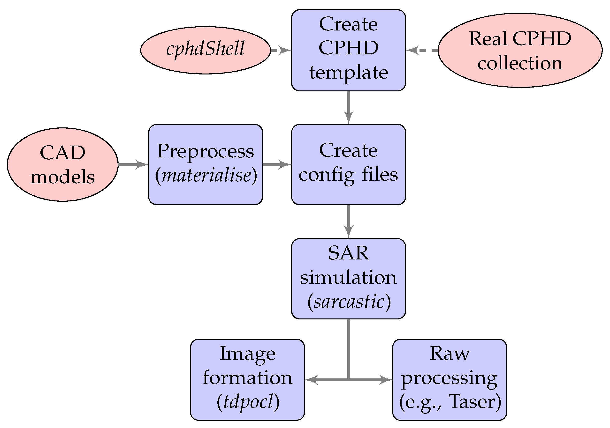
3.1. Framework Overview

SARCASTIC is primarily implemented in C++ and CUDA, along with some utility programs provided as Python scripts. The framework is designed in a modular fashion, allowing new or updated functionality to be integrated easily. The core components are as follows:

• libraytracer—The core raytracing engine;
• sarcastic—The primary SAR simulator;
• bircs—A tool for calculating bistatic RCS values using the raytacing engine, primarily for calibration and regression testing;
• materialise—A tool to introduce surface variations to a CAD model to emulate the surface roughness of the material being modelled;
• SARTrace—A modified version of the SARCASTIC engine which allows the ray history to be enumerated;
• cphdShell—Generates template CPHD data files with zeroed phase history data which are subsequently populated by the SARCASTIC simulator;
• tdpocl—A GPU-accelerated image formation processor used to generate complex SAR images from CPHD data files;
• cphdInfo—Prints summaries of and extracts information from CPHD data files.

Figure 2 shows the typical workflow for a standard SARCASTIC run. The CPHD template file for the simulation contains all necessary metadata to configure the transmitter/receiver RF parameters and collection geometry. CAD models (and their respective materials) constituting the scene can be specified either through the interactive CLI prompt or a JSON scene configuration file. The same is true of the sarcastic configuration options which are passed to the raytracer; a separate JSON configuration file is used for these. This simplifies the process of conducting bulk runs for a set of scenes or configurations through the use of programmatically-generated config files.

3.2. Scattering Model

As the scattering model places fundamental limits on the accuracy and consequent predictive power of the generated SAR data, it is imperative that the model is well-characterised. In addition, it must be possible to explain any discrepancy between the simulator output and an equivalent real result. This almost invariably requires a physically-based approach to be taken, as the assumptions made in modelling the underlying physical mechanisms can be readily quantified and compared to the theoretical ideal results. This can be used to quantify the maximum deviation of the output from the ground truth and inform the implementation of appropriate checks on the result of any subsequent ATR processing.

In this work, an adaptation of Knott’s physical optics model [33] has been developed based on the formula for a flat PEC plate (restated here as Equation (1)). Note that the scattered field amplitude is considered rather than the power, hence the expression for $\sqrt{\sigma }$ as opposed to $\sigma$. This formulation preserves the phase relationship between incident and scattered fields, allowing interference effects to be considered. The nomenclature for Equation (1) and the following derivations is given in

Table 1. Summary of nomenclature used.

Symbol	Explanation	Units
$\sigma$	Radar cross section	$\mathrm{m}$${}^2$
$\widehat{i}$	Incident unit vector	-
$\widehat{s}$	Scattered unit vector	-
$\widehat{n}$	Plate normal unit vector	-
$\widehat{e_r}$	Receiver E-plane unit vector	-
$\widehat{h_i}$	Transmitter H-plane unit vector	-
k	Wavenumber	${\mathrm{m}}^{-1}$
$\overline{r_0}$	Reference range	$\mathrm{m}$
L	Plate length	$\mathrm{m}$
W	Plate width	$\mathrm{m}$
x	Ray-grid length index	-
y	Ray-grid width index	-
z	Ray-grid bounce index	-

.

$$\sqrt{\sigma }=-i\frac{kLW}{\sqrt{\pi }}\widehat{n}·\widehat{e_r}\times \widehat{h_i}{\mathrm{e}}^{\mathrm{ik}\overline{{\mathrm{r}}_0}·\overline{\mathrm{w}}}\times sinc\left[(1/2)\mathrm{k}\overline{\mathrm{L}}·\overline{\mathrm{w}}\right]·sinc\left[(1/2)\mathrm{k}\overline{\mathrm{W}}·\overline{\mathrm{w}}\right]$$

(1)

For notational convenience, we define the vector $\overline{w}$ as follows:

$$\overline{w}=\widehat{i}-\widehat{s}$$

(2)

It is worth studying the form of this result to derive an intuitive, qualitative description of the expected output. The shape of the scattering response is determined by the product of the sinc functions, which are aligned along the local axes of the plate. At normal incidence, maxima in the pattern are observed when the arguments are 0; removing the constants from the expressions shows that this occurs when $\widehat{L}·\overline{w}=0$. This condition is satisfied when $\widehat{i}=\widehat{s}$ (giving $\overline{w}=0$) or when $\overline{w}$ is orthogonal to both $\widehat{L}$ and $\widehat{W}$. Since $\widehat{L}$ and $\widehat{W}$ lie in the plane of the quadrilateral, the condition is satisfied for $\overline{w}=C\widehat{n}$ where C is a scalar constant. From simple geometry, the specular direction for an arbitrary incidence vector is given by

$$\widehat{s}=\widehat{i}-2\widehat{n}\left(\widehat{n}·\widehat{s}\right)$$

(3)

Substituting into Equation (2) and solving for $\overline{w}$ yields

$$\overline{w}=2cos\left(\theta \right)\widehat{n}$$

(4)

and thus a maxima is observed at the specular angle.

A number of potential issues with Equation (1) can be identified by inspection. Knott’s formulation uses a phase term of $ik\overline{r_0}·(\widehat{i}-\widehat{s})$. This is derived by assuming that the signal observed at the receiver is a superposition of reflected plane waves induced by a single incident plane wave with the propagation vector $\widehat{i}$. The fundamental weakness of this approach is that it cannot account for multiple scattering events affecting a single ray, which under the physical optics model become secondary sources emitting a plane wave propagating along the specular direction vector. Furthermore, the target in this case is a single planar surface, not a complex geometry such as would be presented by the CAD model of a real target.

Let us first simplify Equation (1) by removing the constant scaling factors, yielding Equation (5). Instead of treating the incident wave as a single monolithic planar wave, we can model the antenna aperture as a rectangular grid of $x\times y$ ray tubes, each with cross-sectional area $\overline{L_x}\times \overline{W_y}$. Each ray tube can be considered individually and the total RCS arrived at by summation over the grid (Equation (6)). Each ray tube has a number of associated parameters as specified in

Table 2. Ray tube parameters.

Symbol	Explanation	Units
$O_{x,y}$	Ray origin	$\mathrm{m}$
${\widehat{i}}_{x,y}$	Ray propagation vector	-
${\widehat{h_i}}_{x,y}$	Ray H-plane vector	-
$A_{x,y,z}$	Complex amplitude of ray	-
${\sqrt{\sigma }}_{x,y,z}$	RCS contribution seen at receiver	$\mathrm{m}$${}^2$
$d_{x,y,z}$	Distance travelled by ray	$\mathrm{m}$

.

$$\sqrt{\sigma }\propto \widehat{n}·\widehat{e_r}\times \widehat{h_i}{\mathrm{e}}^{ik\overline{r_0}·\overline{w}}\times sinc\left[(1/2)k\overline{L}·\overline{w}\right]·sinc\left[(1/2)k\overline{W}·\overline{w}\right]$$

(5)

$$\sqrt{\sigma }\propto \sum _{x,y}\widehat{n}·\widehat{e_r}\times \widehat{h_i}{\mathrm{e}}^{ik\overline{r_0}·{\overline{w}}_{x,y}}\times sinc\left[(1/2)k\overline{L_x}·{\overline{w}}_{x,y}\right]·sinc\left[(1/2)k\overline{W_y}·{\overline{w}}_{x,y}\right]$$

(6)

Now that each ray can be handled individually, let us consider the case of a CAD model of arbitrary geometry instead of Knott’s single plate. In this case, we can parametrise the facet hit by a ray by its surface normal and the intersection point with the ray, denoted $P_{x,y}$. Note that Knott’s phase term $ik\overline{r_0}·{\overline{w}}_{x,y}$ is obtained by measuring the difference in phase at the intersection point relative to a fixed point on the original plate, $\overline{r_0}$ being the distance between the two points. This definition is now somewhat restrictive, so it is replaced by considering the round-trip distance travelled by a ray, denoted $r_{x,y}$. Combining these changes yields Equation (7).

$$\sqrt{\sigma }\propto \sum _{x,y}{\widehat{n}}_{x,y}·\widehat{e_r}\times \widehat{h_i}{\mathrm{e}}^{{\mathit{ikr}}_{x,y}}\times sinc\left[(1/2)k\overline{L_x}·{\overline{w}}_{x,y}\right]·sinc\left[(1/2)k\overline{W_y}·{\overline{w}}_{x,y}\right]$$

(7)

Now that the model geometry is not planar, we must consider how to address the issue of occlusion. A ray-model interaction should only contribute to the signal at the receiver if there is an unobstructed line of sight between $P_{x,y}$ and the receiver; this is the high-frequency approximation made with PO-based methods. For each ray, the following process is followed:

• Shoot ray from grid into scene;
• If the ray does not hit a model face, record zero contribution and stop;
• Otherwise, shoot a shadow ray from $P_{x,y}$ to the receiver position;
• If the shadow ray intersects a model face, record zero contribution and stop;
• Otherwise, calculate and record the contribution using Equation (7).

Having established a method for decomposing the incident wave and handling arbitrary model geometry, we can now address the problem posed by multi-bounce interactions. Let us expand the intermediate results grid into a third dimension, indexed by the number of interactions between a given ray and the scene model. The summation in Equation (7) is then updated to apply over the new dimension, and the ray tube parameters are re-indexed. The raytracing results can now be stored in a three-dimensional matrix as per Figure 3, where $a_{x,y,z}$ denotes the structure containing a single ray’s data for the z-th interaction with the scene.

To avoid an exponential increase in the number of rays required with each bounce, a geometrical optics approximation is made. After calculating the contribution from the interaction at $P_{x,y,z}$, a new ray is generated with the propagation vector set to the specular direction. The ray is then propagated in the same manner as the original rays from the raygrid. Noting that the polarisation vector of a ray may change due to interactions, we replace $\widehat{h_i}$ with ${\widehat{h}}_{x,y,z}$. We can express the complete contribution calculation as per Equation (8).

$$\sqrt{\sigma }\propto \sum _{x,y,z}{\widehat{n}}_{x,y,z}·\widehat{e_r}\times {\widehat{h}}_{x,y,z}{\mathrm{e}}^{{\mathrm{ikr}}_{x,y,z}}\times sinc\left[(1/2)k\overline{L_x}·{\overline{w}}_{x,y,z}\right]·sinc\left[(1/2)k\overline{W_y}·{\overline{w}}_{x,y,z}\right]$$

(8)

Each ray shot by the simulator is tagged with a number of properties. These include the distance travelled, the phase change and polarisation vector. At each intersection with a model face, the distance travelled by the ray is accumulated and the phase shift/polarisation change is calculated. The shadow rays do not carry a payload as they do not propagate energy through the scene.

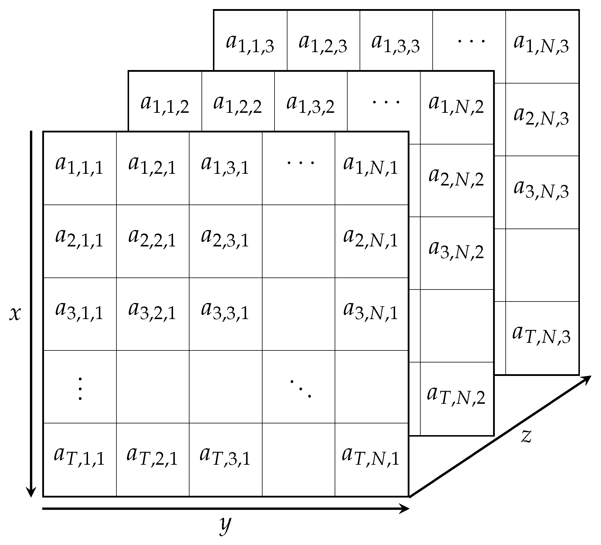
Interpreting the Intermediate Results Matrix

After tracing all rays through the scene, the results matrix as shown in Figure 3 is populated with all calculated contributions to the signal at the receiver. The SARCASTIC raytracer exposes these data to the invoking program. This allows the data to be processed flexibly to produce a wide range of products for analysis.

For example, the results can be directly accumulated into a range profile by inserting each contribution into the relevant bin based on its travelled distance. As all reflections are recorded in terms of $\sqrt{\sigma }$, which is by definition complex, the equivalent phasor can be rotated by the relative phase shift due to reflections and accumulated into the bin. This directly accounts for interference effects, and gives a profile suitable for storage as phase history data. A point spread function with the appropriate resolution as calculated from the collection metadata is then convolved with the raw profile before storage.

Alternatively, selection criteria can be used to filter the contributions from the intermediate matrix which are used to form the range profiles. This could be as simple as all contributions which result from two interactions only ($\sum a_{x,y,2}$), or all multipath returns (${\sum }_{1<z}{a}_{x,y,z}$). When investigating the response from an individual scatterer or feature, a filter could be constructed by considering the expected round-trip distance to the target, selecting only the rays which relate to interactions occurring within the slant-range bins which intersect a bounding box containing the feature. In the SARtrace utility, the facet hit on each ray-model interaction is stored and can be used to select the contributions resulting from specific pieces of the scene geometry.

3.3. Data Formats

SARCASTIC outputs results in compensated phase history data (CPHD) format. In the original release, this was written to/read from one of two file formats (CPHD V3.0 2008 or CPHD X V0.3) via homebrew functionality in the SAR C Library (sarclib). This implementation was incomplete and did not exploit several major features provided by the standards. It also did not support the latest NGA.STAN.0068-1 standards, which were released in 2016 and 2018 respectively.

CPHD support is now provided through the official Sensor-Independent XML (SIX) library from the US National Geospatial-Intelligence Agency. Support for the CPHD V3.0 2008 standard has been discontinued, and CPHD X V0.3 is the current default in SARCASTIC v2.0. Ongoing work aims to integrate the latest NGA.STAN.0068-1 V1.0.1 format as well, which will open up several exploitation avenues that were not possible in SARCASTIC’s previous configuration. In particular, electronic beamsteering, multiple stabilisation reference points, and atmospheric propagation correction factors can be incorporated into the CPHD products.

3.4. Building for High-Throughput Applications

As previously discussed, the primary challenge to effective ATR research is typically not the accuracy of the available data, but rather its volume. In order to ensure that SARCASTIC is capable of achieving and maintaining high throughput across its operating envelope, it was decided at an early stage in the project to establish a development approach which complemented this aim. The formal requirements for SARCASTIC v2.0 explicitly stated that parallel computation and hardware acceleration would be exploited wherever possible and appropriate in order to reduce the run-time of the simulator, and that:

• Any reduction in accuracy or fidelity of the result will be flagged to the user, and an option to disable the optimisation made available;
• Code will be written in such a manner that the acceleration scales with the number of available processors and availability of required resources (e.g., RAM, I/O bandwidth, etc.);
• Nvidia GPUs will be targeted specifically. A compute capability of ≥$2.0$ will be assumed.

3.4.1. Preprocessing Steps

As shown in Section 3.1, the CAD models to be used in a SARCASTIC simulation may be preprocessed with the materialise utility to introduce rough surfaces. Time consumed in this step increases the cycle time when running iterative simulations, so it is desirable to reduce the runtime of these preprocessing utilities. Consider an example run on the Athens compute server at UCL for a M1133 Stryker model containing 188,714 faces. The segmentation step for the original release takes 36 $\min$ $25.28$ $\mathrm{s}$; in the v2.0 release, the equivalent process takes $19.46$ $\mathrm{s}$, a 99.11% reduction in processing time.

The original materialise used a custom implementation of a half-edge triangle mesh, and traversed it inefficiently by performing a complete copy-and move of the whole mesh at least once on every segment. The number of iterations was very high, as a strict equality of normals between neighbouring faces was required to combine faces into a segment prior to Delaunay triangulation. The average number of faces in a segment for one test was 3 on a Leopard 2A6 tank model with 155,462 faces.

The current improvements were gained by switching to the half-edge mesh implementation provided by the Point Cloud Library (PCL), and writing an efficient traversal algorithm which operates on a single in-place copy of the data whilst using std::vector queues to track progress. OpenMP is used to divide the Delaunay triangulation tasks for each section across all available cores, and the results for each segment are then merged by a single thread to complete the final model for output.

3.4.2. GPU Acceleration

The scattering model described in Section 3.2 is eminently suitable for parallelisation via implementation on GPUs. Each entry in the ray-grid matrix is only dependent on the entry for the previous bounce level and/or global parameters. Within the supporting raytracer, it is desirable to model this as a causal but non-recursive relationship, thus eliminating the need for a stack on the GPU to track recursion. Instead, the parameters for each ray are stored in the globally-accessible intermediate results matrix described in Section 3.2; on completion of a ray-facet interaction calculation, a new ray is launched for the specular reflection using parameters initialised with the results from the previous interaction.

The NVIDIA OptiX library was selected as meeting the criteria outlined above. Whilst this does reduce the portability of the software, it was determined that the target compute environments would almost certainly be using CUDA for other processing already and thus have suitable GPUs available. The ability to directly interleave CUDA pre/post-processing with the primary raytracing operations is another factor which influenced this choice.

During a simulation run, the CAD models comprising the target scene are loaded by OptiX into its internal bounding volume hierarchy acceleration structures. For each pulse in the SAR collection, a host-side routine calculated the appropriate positioning of the receiver/transmitter platforms and the sizing of the required ray grid. These data are then used to initialise an OptiX run, which launches and propagates all the rays through the scene for the specified number of interactions. The intermediate results matrix is held in device memory for post-processing via CUDA routines launched by the host.

The conversion to range profiles is achieved using a CUDA kernel which constructs profiles from a subset of the rays in the ray-grid and subsequently column reduces across the array of sub-profiles to produce the complete profile for all contributions. This is then convolved with a point response function to produce the final range profile which is returned from device memory to the host. The cost of this final copy is trivial compared to the potential cost of directly transferring the ray-grid matrix from the device to host memory.

In multi-GPU systems, it is possible to parallelise multiple simulation runs by launching each run with a separate CUDA context which is only aware of a single GPU. This prevents OptiX preforming unnecessary device-to-device copies and reduces the PCI-E bandwidth usage per run.

4. Results

This section presents a selection of results obtained using the SARCASTIC v2.0 simulator, demonstrating its capabilities and versatility in addressing a range of complex problems. Where image formation results are shown, these have been constructed using the tdpocl utility and the Taser tool from the MATLAB SAR toolbox [34]. All CAD models are prepared using standard open-source packages such as Blender.

One of the key issues identified with SARCASTIC v1.0 was that the scattering model was not guaranteed to produce consistent results for different polarisations. As shown in Section 3.2, the new scattering model addresses this issue by tracking the polarisation and complex amplitude of each ray throughout the scene. A number of bircs simulations were carried out to test the polarisation dependence for the new model, using a PEC dihedral target.

The two plates forming the target were of side length 1 $\mathrm{m}$ and the incident illumination was set to a frequency of 10 $\mathrm{G}$$\mathrm{Hz}$. The ray-tube side length was set at $0.05\lambda$. The difference between the calculated monostatic responses for VH and HV is shown in Figure 4; clearly, the error is within acceptable bounds.

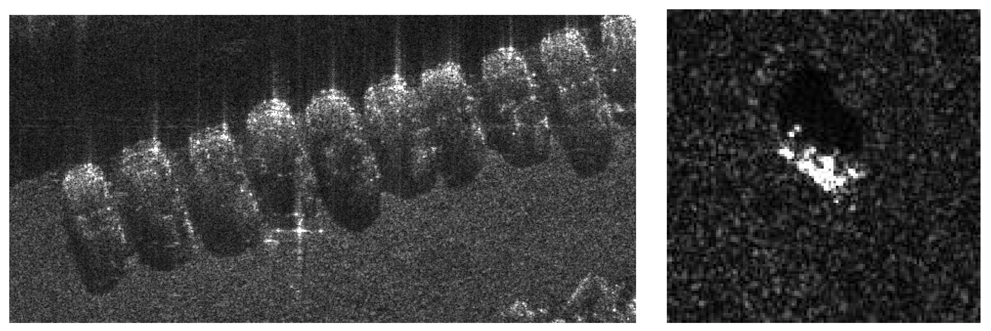
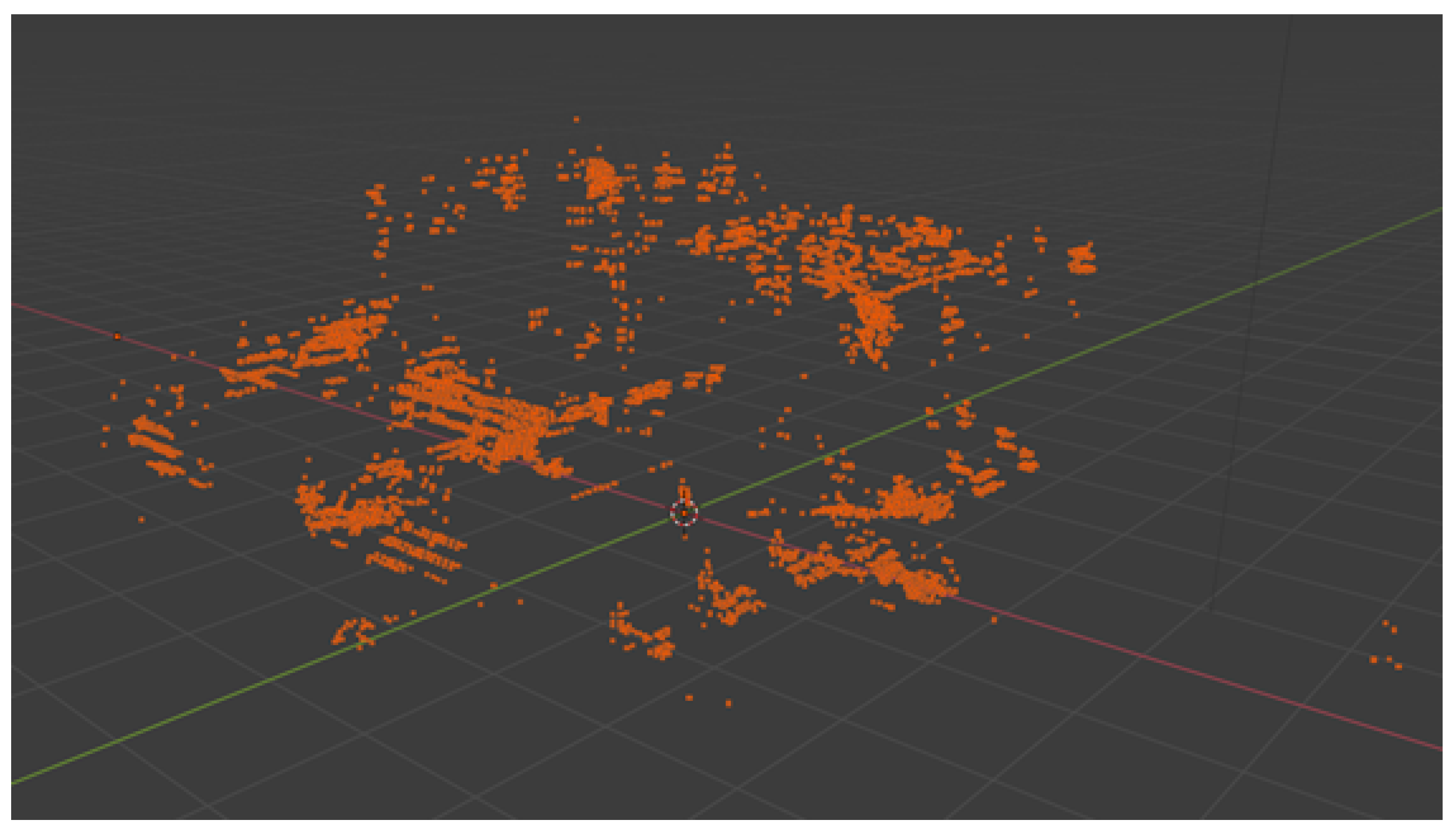
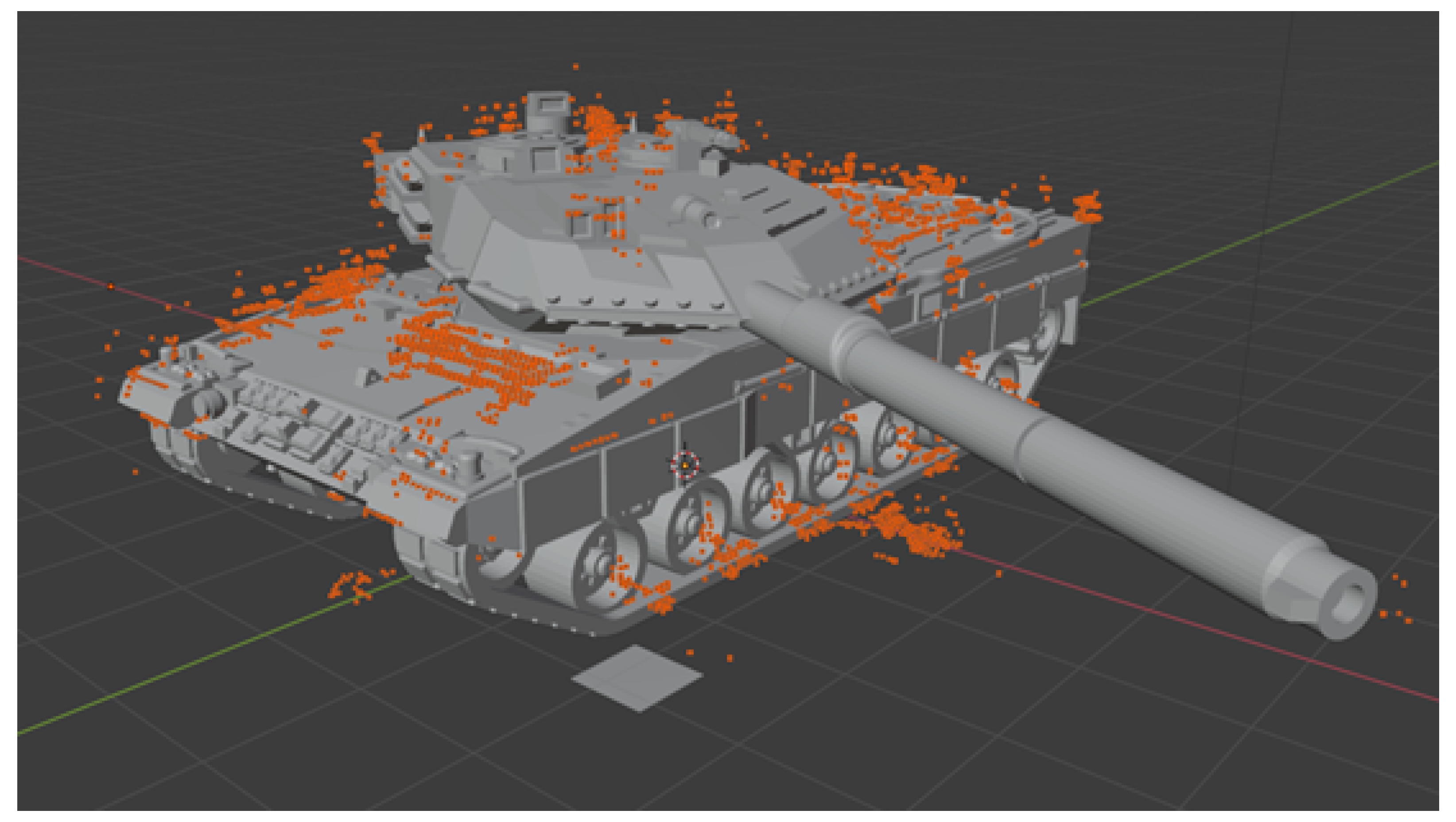
4.1. 3D Point Cloud Extraction

An effective demonstration of the utility of SARCASTIC simulations is through their use to assess the fidelity of 3D point cloud reconstructions from a number of SAR images obtained at different incidence angles. The processing uses the complex SAR images and it is essential that the correct phase relationships have been incorporated in the simulations for successful point cloud extraction.

For 3D point cloud formation [35], SAR images are formed from platforms at a number of different incidence angles. One of the incidence angles is taken as the “reference” image and the others are taken as “secondary” images. The phase differences in “corresponding” pixels between each secondary image and the reference image are required. These are then compared with the phase differences which would be expected at different heights to find the best match.

This is illustrated in Figure 5 for two platforms. Imagine that there is a point target at the top end of the smaller double headed red arrow. This scatterer is at height $\mathsf{\Delta }h$. When imaged, the target is assumed to be on the ground and so will appear where the circular arc centred on the lower satellite intersects the ground as this is the ground position which has the same range as the target. This position will be referred to as the layover point which will be at a distance $\mathsf{\Delta }htan\psi$ from the actual ground range position of the target, where $\psi ={90}^{\circ }-\theta$. There will be a difference (which will be referred to as a “delta” to help with the explanation) in the ranges to the layover point between the lower and upper satellites which will result in a phase delta between the complex pixel values associated with this point in the two images.

Consider now the ranges from the two satellites to the point target. There will again be a delta between the two ranges which will result in a phase difference which can be measured between the two images. The key point is that there will be a difference between the delta in range at the layover point and at the point target which will depend on the height. In the diagram, a circular arc centred on the upper satellite has been drawn to show all ranges that are the same as the range to the layover point. It can be seen that the difference in the range deltas is given by $\mathsf{\Delta }r$ where [36]

$$\mathsf{\Delta }r=\frac{B_{\perp }}{r_{0}sin\theta }\mathsf{\Delta }h$$

(9)

Thinking in terms of incidence angles and noting $B_{\perp }=r_0\varphi$, it then transpires that

$$\mathsf{\Delta }r=\frac{\mathsf{\Delta }\varphi }{cos\varphi }\mathsf{\Delta }h$$

(10)

where $\mathsf{\Delta }\varphi$ is the angular delta between the slant range directions to the point target from the two satellites. It is important to emphasise that this refers to a difference in range deltas, and that the range deltas are associated with the point target and the layover point of that point target.

Given K platforms, the measured phase ${\varphi }_{k,meas}$ can be compared with the anticipated phase for a given height through the Measured Interferometric Response Function (MIRF)

$$mirf\left(h\right)=\frac{1}{K}\left|1+\sum _{k=1}^{K-1}exp\left({\varphi }_{k,meas}-2\pi i\frac{\mathsf{\Delta }r}{\lambda }\right)\right|$$

(11)

The MIRF will take a value of 1 if the measured phases exactly match the phases anticipated for a given height but will take lower values when the phases are mismatched. If regular incidence angle separation is used then the MIRF will contain grating lobes (regular repeats of the main peak) which will introduce ambiguities in the height estimation. For this reason, non-regular incidence angle separations are to be preferred. There will still be a maximum range of unambiguous heights determined by the range of incidence angles spanned. Detailed discussion of these considerations is beyond the scope of this paper.

Given the reference image and the secondary images, point cloud processing proceeds by calculating the MIRF as a function of height at each pixel position. There is an important point to note here. It is the phases associated with a particular point target that are required for point cloud processing. However, because of layover, the point target will appear at different range positions in the image depending on the different incidence angles. Thus it is necessary to track the point target through the images. The variation of the layover range will depend on the target height. If the height were known, then the position of the target could be anticipated, but of course the whole point is to estimate the height. The solution is to step through postulated heights, shift the images so that any scatterers at this height will be aligned and then calculate the MIRF value for that height.

This processing will result in a 3D array of MIRF values defined for range and azimuth pixel positions and for height. The MIRF values will be in the range [0, 1] with values close to 1 indicating that the phases across the images are consistent with there being a point scatterer at that position and height. Sometimes, random noise fluctuations can produce MIRF values close to 1 and so it is convenient to weight the MIRF values by the actual image values. In this way, to declare a point scatterer to be at a given position and height it is necessary for the MIRF value to be close to 1 and the image value at that position to be bright. For the results presented here, the weighting has been achieved by raising the MIRF values to the eighth power and multiplying by the log of the image. Thresholds relative to the maximum value can then be set to extract point scatterers. A detailed analysis of optimising this process is beyond the scope of this paper.

In the following examples, a SAR system operating at 10 $\mathrm{G}$$\mathrm{Hz}$ has been simulated. The reference incidence angle is 25 degrees. The azimuth and ground range resolutions are $0.1$ $\mathrm{m}$ and image sampling is at $0.05$ $\mathrm{m}$. In all images, the illumination is from the bottom. Results are shown using Blender 3D and illumination in these figures is towards the negative x direction.

The first example considers a SARCASTIC simulation of a set of seven trihedrals. The reference image resulting from this simulation is shown in Figure 6. The trihedrals are separated from each other by 10 $\mathrm{m}$ in azimuth and 10 $\mathrm{m}$ in ground range. The leftmost trihedral in Figure 6 is at ground level and then moving from left to right, the trihedral heights increase by $0.5$ $\mathrm{m}$ each time. It can be seen that, as the height increases, the trihedrals appear at a closer range than their actual position as the image has been formed at zero height and so there is an increasing layover effect.

Three secondary images were used for point cloud processing at incidence angles of 25.2, 25.6 and 25.7 degrees. The output from point cloud processing compared to the input CAD model is shown in Figure 7. A suitable threshold has been chosen to display only the strongest candidate scatterers. It can be seen that point scatterers have been extracted at positions corresponding to the apex of each trihedral. There are two additional points close to the central trihedral which will have resulted from sidelobe structures. This result provides strong validation that accurate phase relationships are being produced by SARCASTIC as it is allowing very accurate point cloud reconstruction using a well-characterised scattering object, i.e., a trihedral.

The second example considers a SARCASTIC simulation of an electricity pylon. The CAD model for the electricity pylon is shown in Figure 8a and the SAR (reference) image resulting from the SARCASTIC simulation is shown in Figure 8b. The pylon is actually positioned right at the upper edge of the image so that all returns from the pylon are contained within the image extent despite the layover effect. It can be seen that the pylon is a complex structure which results in an image which is difficult to interpret.

Point cloud processing has been performed using three secondary images with incidence angles of 25.06, 25.18 and 25.21 degrees. Figure 9a shows a height slice at 4.8 m from the weighted MIRF whilst Figure 9b shows a detail of the pylon with the extent of the slice indicated by a horizontal plane. The point cloud slice appears to show scattering from the two angular structures formed near the centre of the front of the pylon (i.e., the side facing the illumination which is in the direction of negative x). Similar scattering from the back of the pylon is just visible although it is just at the edge of the image extent. There is also scattering from the structures at the centres of the two sides. Finally there appears to be significant scattering, extended in the azimuth direction, from the back of the pylon. Figure 10a shows a height slice at 20.7 m from the weighted MIRF whilst Figure 10b shows the corresponding detail of the pylon. It can be seen that there are strong scattering events associated with eight instances where vertical and horizontal structures meet. It is interesting to note that similar strong scattering is not observed for the four innermost instances where vertical and horizontal structure meet. Figure 11a shows a height slice at 23.5 m from the weighted MIRF whilst Figure 11b shows the corresponding detail of the pylon. Similar observations to the preceding paragraph can be made although, in this case, the scattering from the back of the pylon is more extended. Whilst these results reveal scattering events which need more careful consideration to understand fully, it is clear that the information provided by the point cloud processing is associated with the structures observed at the associated height. This again validates the phase relationships which are simulated by SARCASTIC in this more complex scattering example.

The final example considers a SARCASTIC simulation of a Leopard tank. Figure 12 shows the SAR (reference) image resulting from the SARCASTIC simulation. A further seven imaging geometries were considered where the angle between the illumination and the Leopard tank was varied by 45 degrees each time. Corresponding secondary images were simulated using incidence angles of 25.2, 25.6 and 25.7 degrees. Point cloud processing was applied for each of the eight different geometries and the resulting point clouds were combined. The final combined point cloud is shown in Figure 13 and is shown together with the CAD model of the Leopard tank in Figure 14. It is clear that the point cloud processing provides significant additional information in terms of 3D structures in comparison to the 2D SAR image. Certainly the wheel structures, hull shape and the end of the barrel can be discerned. Whilst this example does not necessarily provide further validation of SARCASTIC, it does show how SARCASTIC can be used to support performance analysis. In this case, it is of interest to quantify the benefits in terms of recognition performance of having 3D point cloud information available. It is not feasible to collect sufficient real SAR data to support this analysis. However, it has been seen that SARCASTIC provides accurate phase relationships in its simulations which allow point clouds to be extracted. It can thus be used to generate large numbers of examples which can be used to support target recognition performance analysis. This is the subject of ongoing work.

4.2. Scattering Investigations with SARTrace

As discussed in Section 3.1, the SARCASTIC framework contains a number of additional tools for inspection and analysis of the simulation process. SARTrace is commonly use to locate scattering mechanisms within a scene which give rise to a visible feature in the matching SAR imagery.

An example visualisation is shown in Figure 15a; the target and capture geometry are as shown in the multipath investigation of [16]. This image was created by rendering the SARTrace PLY file output for the first bounce of a single pulse in Blender. Figure 15b shows the same result from a different angle, clearly illustrating that the facets on the shadowed side of the model have not been illuminated. Other areas no expected to receive direct illumination, such as the lower side of the sloped armour at the front of the turret, are also absent from the model. The shadow cast onto the right side armour by the overhanging turret is clearly visible; note that it occludes the central road wheel, which would give a strong trihedral-like response in SAR imagery if illuminated.

Figure 15c shows the same visualisation as Figure 15a with the second bounce interactions overlaid in green. This output shows that several previously shadowed surfaces have been indirectly illuminated via multipath interactions. In particular, the lower front sections of the turret and the outer surfaces of the middle road wheel are now hit by rays and may contribute to the signature. In this image, potions of the belly are also shown as being intersected by rays, indicating that the sections of track on the vehicle’s right side are illuminating it via specular reflection (there is no ground plane/terrain in the simulation shown). SARTrace can be configured to select only facets which contribute to the total RCS at a given bounce level. In that case, we would expect the belly section to be eliminated as there is no valid line-of-sight to the receiving antenna phase centre from those facets.

Inspection of SARTrace results can also be used to refine a simulation by identifying issues with the models used or the raytracing parameters chosen. In this example, it could be determined that the ray tube side length is sufficiently small to achieve good coverage of the top and side armour. However, it is probably too high for detailed analysis of multipath analysis in the road wheel/track regions; some facets where interactions would be expected appear to have been missed on the second bounce.

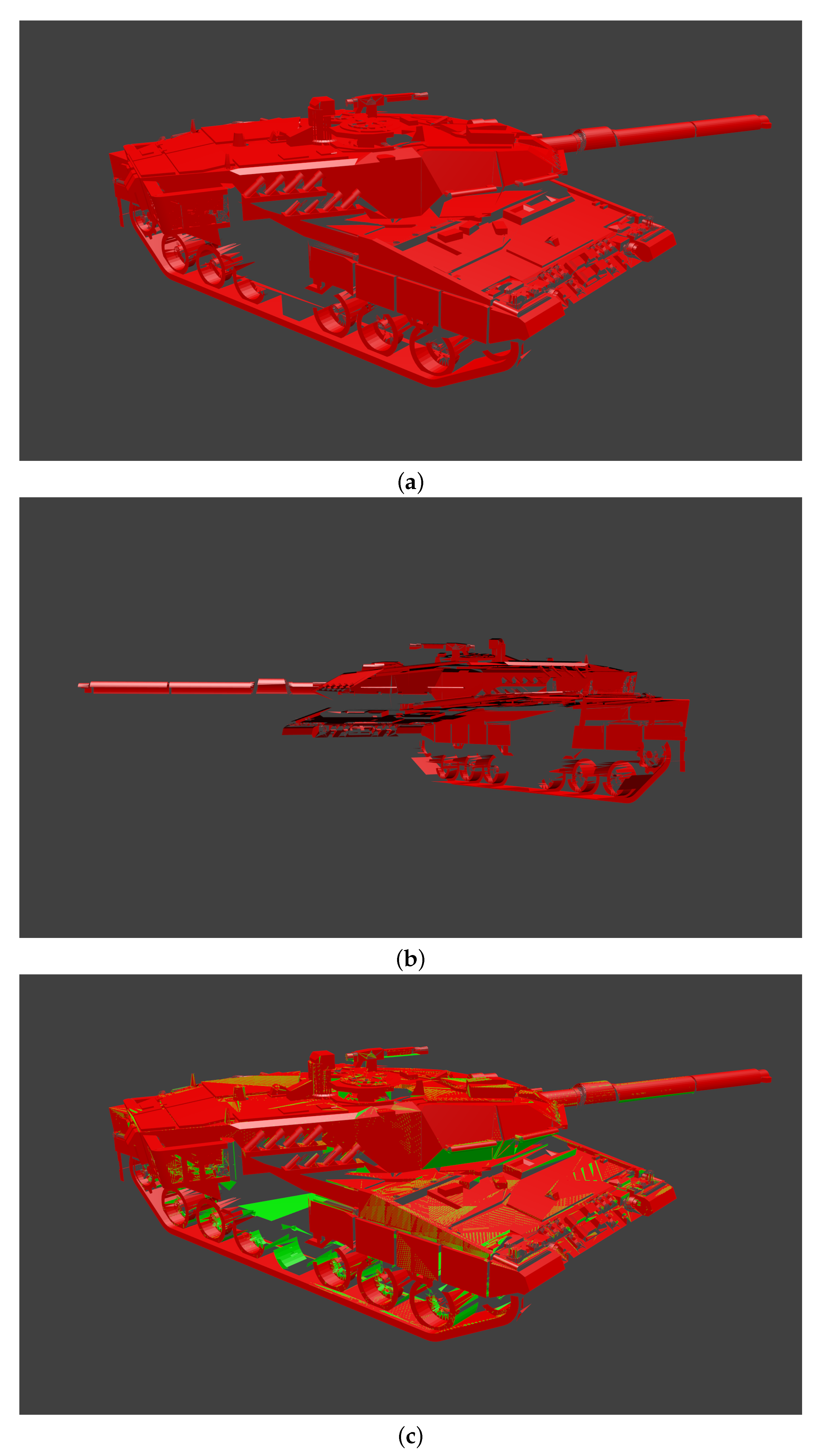
4.3. Generating a Data Dome for Vehicular Targets

The data dome approach is commonly used to characterise a single target, such as a vehicle or small structure, over a wide range of aspect angles. Comprehensive simulated results generated by Xpatch have been released for a small number of civilian vehicles [30,37]. Such datasets are invaluable for ATR research, as they offer good coverage across the observation angles at which a sensor system is likely to encounter the class and allow aspect-dependent phenomena to be investigated.

An example data dome for a T-72B has been generated using SARCASTIC v2.0, and can be accessed at https://doi.org/10.5522/04/c.5892392 (accessed on 20 May 2022). This dataset includes both CPHD files and reconstructed images. A slant-range and azimuth resolution of 15 cm has been chosen for this dataset, representing a significant improvement over MSTAR. To improve the availability of ATR training data, it is intended that future projects will generate similar datasets for a wide range of target models and operating conditions. The authors welcome suggestions from the radar community regarding target classes and scenarios of particular interest.

4.4. Runtime Performance Analysis

The following results illustrate the performance of SARCASTIC v2.0 under typical operating conditions. The focus is on the runtime of the sarcastic executable. Improvements in model preparation time have been addressed previously in Section 3.4.

To demonstrate the near-realtime performance which can be achieved with SARCASTIC, an example CPHD collection was simulated with representative parameters suitable for a high-resolution airborne SAR system. The sensor was moving along a stripmap aperture at 50 $\mathrm{m}{\mathrm{s}}^{-1}$ with a mean pulse repetition frequency of 100 $\mathrm{Hz}$ and a total bandwidth of 1836 $\mathrm{M}$$\mathrm{Hz}$. The grazing angle was $35.3^{°}$ at the centre of the synthetic aperture. The time required to fly through the complete aperture is $22.5$ $\mathrm{s}$ during which 2250 pulses are required to form an image with a resolution of 10 $\mathrm{c}$$\mathrm{m}$ (ground range) × $6.9$ $\mathrm{c}$$\mathrm{m}$ (azimuth).

A SARCASTIC run using this configuration and $0.5\lambda$ ray-tube sizing against the Leopard 2A6 target model shown in Figure 14 completes in $17.741$ $\mathrm{s}$. The resulting output accounts for up to 4 multi-bounce interactions per ray, giving good visual matches for expected di/trihedral structures and other strong scattering centres. Reducing the ray-tubes to $0.25\lambda$ for greater fidelity around smaller scattering features increases the runtime by 199%, completing in $53.060$ $\mathrm{s}$. A complete characterisation of the performance across the configuration parameter space is beyond the scope of this paper but will from the basis of a subsequent publication.

As noted previously, the high throughput of SARCASTIC is a key enabler for generating datasets of sufficient size to support ATR research. Let us consider a practical example such as the generation of the T72-B data dome in Section 4.3. In the worst case, we assume that a complete stripmap collection must be simulated for each azimuth, elevation combination in the data dome.

The data dome covers 24 azimuth and 7 elevation angles, giving 168 files. Each CPHD file contains 720 pulses yielding 120,960 profiles in total for the dome. The bulk run to generate these data required 1459 $\mathrm{s}$ of wallclock time when 2 V100 GPUs were used. This is equivalent to $24.124$ $\mathrm{m}$$\mathrm{s}$ per profile. These results were obtained on a shared compute server whilst other tasks were running, and therefore represent a lower bound on the achievable throughput for the stated hardware.

This improves on the Xpatch results calculated in Section 2.5 by a factor of 4, and requires a fraction of the hardware. Early trials with the SARCASTIC v1.0 simulator achieved runtimes of approximately 700 $\mathrm{m}$$\mathrm{s}$ per pulse for similar simulations [16]. Note that SARCASTIC v1.0 was CPU-bound rather than GPU-bound, so the hardware requirements to achieve that performance were significantly different (enterprise-grade CPU compute node).

For comparative purposes, the RaySAR pipeline previously used by the authors for ATR research [15] was capable of generating approximately 5000 images per node per hour on the Legion and Myriad HPC clusters at UCL. It is not possible to directly compare the performance of RaySAR and SARCASTIC because they generate fundamentally different data (contribution maps/image chips vs. whole aperture phase history). Many images can be generated from a single CPHD file through techniques such as sub-aperture construction.

5. Conclusions and Future Work

This paper presents a major upgrade to the SARCASTIC simulation and analysis framework, delivering significant improvements in accuracy and runtime performance. Practical examples of its application to a number of complex modelling and analysis problems have been demonstrated. In particular, it has been shown that the simulator is capable of handling complex target models for arbitrary collection geometries, and that the phase history output is accurate and consistent across multiple discrete runs. This has been confirmed through the application of interferometric processing to a set of CPHD output files.

It has been demonstrated that SARCASTIC now has the potential to break the deadlock in SAR ATR research by generating the required training data at a suitable scale and fidelity. This is a fundamental enabler for applying modern deep learning and image understanding methods to the SAR problem space. By pursuing a straightforward methodology and scattering model based on well-established electromagnetic theory, data produced using this simulator can be released into the public domain without the constraints associated with other established programs such as Xpatch. As noted in Section 4.3, demand from the wider radar community for datasets covering targets or scattering phenomena of particular interest will be a key driver for the generation of standardised data releases.

The SARCASTIC modelling approach does not currently account for more complex electromagnetic phenomena such as diffraction and travelling waves. There are several well-known methodologies for introducing such considerations to SBR-based simulators. A popular method based on edge waves is the implementation of incremental length diffraction coefficients [38]; this approach has been used in other published radar simulators such as SigmaHat [39].

A trial is currently being conducted by Dstl to validate SARCASTIC outputs against data from a range of real SAR sensors. This project will lay the foundation for investigating SARCASTIC’s application to interrogating collections displaying unintuitive phenomenology, such as multipath interactions for non-canonical targets. Prior work by Muff using SARCASTIC v1.0 and data from the Hydravision II trial showed promising results in this area [22].

Future work will focus on the application of this simulation engine to novel and challenging remote sensing problems in the SAR domain. Particular attention will be paid to problem spaces where the lack of existing data has previously limited research activity. Example use cases include signature database generation for investigations of ATR performance under extended operating conditions or bistatic geometries [16], automated scene reconstruction and data fusion between multiple discrete SAR platforms.

Development of new technologies in the remote sensing field is heavily dependent on the availability of representative data; the non-intuitive phenomenology presented by SAR systems is particularly challenging to predict. Complex post-processing techniques such as ATR require exceptionally large volumes of sample date for development, testing and validation before deployment; typically, such campaigns can only be supported through simulators such as SARCASTIC. This is especially true when novel operating modes or sensor configurations are under consideration, and no existing platform can provide relevant data in sufficient volume. The updated approach that has been demonstrated in this paper will ensure that these avenues can be explored, de-risking the development and deployment of new technologies for next-generation SAR systems.

References

1. Sherwin, C.W.; Ruina, J.; Rawcliffe, R. Some early developments in synthetic aperture radar systems. IRE Trans. Mil. Electron. 1962, 1051, 111–115. [Google Scholar] [CrossRef]
2. El-Arnauti, G.; Saalmann, O.; Brenner, A.R. Advanced System Concept and Experimental Results of the Ultra-High Resolution Airborne SAR Demonstrator PAMIR-Ka. In Proceedings of the EUSAR 2018, 12th European Conference on Synthetic Aperture Radar, Aachen, Germany, 4–7 June 2018; pp. 1–5. [Google Scholar]
3. Ignatenko, V.; Laurila, P.; Radius, A.; Lamentowski, L.; Antropov, O.; Muff, D. ICEYE Microsatellite SAR Constellation Status Update: Evaluation of first commercial imaging modes. In Proceedings of the 2020 IEEE International Geoscience and Remote Sensing Symposium, Virtual, 26 September–2 October 2020; IEEE: Piscataway, NJ, USA, 2020; pp. 3581–3584. [Google Scholar]
4. Ignatenko, V.; Nottingham, M.; Radius, A.; Lamentowski, L.; Muff, D. ICEYE Microsatellite SAR Constellation Status Update: Long Dwell Spotlight and Wide Swath Imaging Modes. In Proceedings of the 2021 IEEE International Geoscience and Remote Sensing Symposium, Virtual, 12–16 July 2021; IEEE: Piscataway, NJ, USA, 2021; pp. 1493–1496. [Google Scholar]
5. The Air Force Moving and Stationary Target Recognition Database. Available online: https://www.sdms.afrl.af.mil/index.php?collection=mstar (accessed on 20 November 2021).
6. Malmgren-Hansen, D.; Nobel-J⊘rgensen, M. Convolutional neural networks for SAR image segmentation. In Proceedings of the 2015 IEEE International Symposium on Signal Processing and Information Technology (ISSPIT), Abu Dhabi, United Arab Emirates, 7–10 December 2015; IEEE: Piscataway, NJ, USA, 2015; pp. 231–236. [Google Scholar]
7. Stevens, M.; Jones, O.; Moyse, P.; Tu, S.; Wilshire, A. Bright Spark: Ka-band SAR technology demonstrator. In Proceedings of the International Conference on Radar Systems (Radar 2017), Belfast, UK, 23–26 October 2017; IET: London, UK, 2017; pp. 1–4. [Google Scholar]
8. Potin, P.; Rosich, B.; Grimont, P.; Miranda, N.; Shurmer, I.; O’Connell, A.; Torres, R.; Krassenburg, M. Sentinel-1 mission status. In Proceedings of the EUSAR 2016: 11th European Conference on Synthetic Aperture Radar, Hamburg, Germany, 6–9 June 2016; VDE: Frankfurt, Germany, 2016; pp. 59–64. [Google Scholar]
9. Lewis, B.; DeGuchy, O.; Sebastian, J.; Kaminski, J. Realistic SAR data augmentation using machine learning techniques. In Algorithms for Synthetic Aperture Radar Imagery XXVI; International Society for Optics and Photonics, SPIE: Bellingham, WA, USA, 2019; Volume 10987, pp. 12–28. [Google Scholar]
10. Inkawhich, N.; Inkawhich, M.J.; Davis, E.K.; Majumder, U.K.; Tripp, E.; Capraro, C.; Chen, Y. Bridging a Gap in SAR-ATR: Training on Fully Synthetic and Testing on Measured Data. IEEE J. Sel. Top. Appl. Earth Obs. Remot. Sens. 2021, 14, 2942–2955. [Google Scholar] [CrossRef]
11. Lewis, B.; Scarnati, T.; Sudkamp, E.; Nehrbass, J.; Rosencrantz, S.; Zelnio, E. A SAR dataset for ATR development: The Synthetic and Measured Paired Labeled Experiment (SAMPLE). In Algorithms for Synthetic Aperture Radar Imagery XXVI; International Society for Optics and Photonics: Bellingham, WA, USA, 2019; Volume 10987. [Google Scholar]
12. degaard, N.; Knapskog, A.; Cochin, C.; Delahaye, B. Comparison of real and simulated SAR imagery of ships for use in ATR. In Algorithms for Synthetic Aperture Radar Imagery XVII; International Society for Optics and Photonics: Bellingham, WA, USA, 2010; Volume 7699. [Google Scholar]
13. Auer, S.; Hinz, S.; Bamler, R. Ray-tracing simulation techniques for understanding high-resolution SAR images. IEEE Trans. Geosci. Remot. Sens. 2010, 48, 1445–1456. [Google Scholar] [CrossRef] [Green Version]
14. Auer, S.; Bamler, R.; Reinartz, P. RaySAR-3D SAR simulator: Now open source. In Proceedings of the 2016 IEEE International Geoscience and Remote Sensing Symposium, Beijing, China, 10–15 July 2016; IEEE: Piscataway, NJ, USA, 2016; pp. 6730–6733. [Google Scholar]
15. Woollard, M.; Bannon, A.; Ritchie, M.; Griffiths, H. Synthetic aperture radar automatic target classification processing concept. Electron. Lett. 2019, 55, 1301–1303. [Google Scholar] [CrossRef]
16. Woollard, M.; Ritchie, M.; Griffiths, H. Investigating the effects of bistatic SAR phenomenology on feature extraction. In Proceedings of the 2020 IEEE International Radar Conference (RADAR), Washington, DC, USA, 28–30 April 2020; IEEE: Piscataway, NJ, USA, 2020; pp. 906–911. [Google Scholar]
17. Chatzigeorgiadis, F.; Jenn, D.C. A MATLAB physical-optics RCS prediction code. IEEE Antennas Propag. Mag. 2004, 46, 137–139. [Google Scholar]
18. Chatzigeorgiadis, F. Development of Code for a Physical Optics Radar Cross Section Prediction and Analysis Application; Naval Postgraduate School: Monterey, CA, USA, 2004. [Google Scholar]
19. Ludwig, A. Computation of radiation patterns involving numerical double integration. IEEE Trans. Antennas Propag. 1968, 16, 767–769. [Google Scholar] [CrossRef]
20. Ludwig, A.C. Calculation of Scattered Patterns From Asymmetrical Reflectors; University of Southern California: Los Angeles, CA, USA, 1969. [Google Scholar]
21. Moreira, F.J.; Prata, A. A self-checking predictor-corrector algorithm for efficient evaluation of reflector antenna radiation integrals. IEEE Trans. Antennas Propag. 1994, 42, 246–254. [Google Scholar] [CrossRef]
22. Muff, D.G. Electromagnetic Ray-Tracing for the Investigation of Multipath and Vibration Signatures in Radar Imagery. Ph.D. Thesis, UCL (University College London), London, UK, 2018. [Google Scholar]
23. Muff, D.G.; Andre, D.; Corbett, B.; Finnis, M.; Blacknell, D.; Nottingham, M.R.; Stevenson, C.; Griffiths, H. Comparison of vibration and multipath signatures from simulated and real SAR images. In Proceedings of the International Conference on Radar Systems (Radar 2017), Belfast, UK, 23–26 October 2017. [Google Scholar]
24. Cochin, C.; Pouliguen, P.; Delahaye, B.; le Hellard, D.; Gosselin, P.; Aubineau, F. MOCEM—An “all in one” tool to simulate SAR image. In Proceedings of the 7th European Conference on Synthetic Aperture Radar, Friedrichshafen, Germany, 2–5 June 2008; VDE: Frankfurt, Germany, 2008. [Google Scholar]
25. Cochin, C.; Louvigne, J.C.; Fabbri, R.; Le Barbu, C.; Ferro-Famil, L.; Knapskog, A.O.; Odegaard, N. MOCEM V4 - Radar simulation of ship at sea for SAR and ISAR applications. In Proceedings of the EUSAR 2014: 10th European Conference on Synthetic Aperture Radar, Berlin, Germany, 3–5 June 2014; VDE: Frankfurt, Germany, 2014; pp. 608–611. [Google Scholar]
26. Knapskog, A.O.; Vignaud, L.; Cochin, C.; Odegaard, N. Target Recognition of Ships in Harbour Based on Simulated SAR Images Produced with MOCEM Software. In Proceedings of the EUSAR 2014: 10th European Conference on Synthetic Aperture Radar, Berlin, Germany, 3–5 June 2014; VDE: Frankfurt, Germany, 2014; pp. 1188–1191. [Google Scholar]
27. Vignaud, L.; Odegaard, N.; Ruggiero, H.; Cochin, C.; Louvigne, J.C.; Knapskog, A.O. Comparison of simulated and measured ISAR images flow of a ship at sea. In Proceedings of the EUSAR 2021: 13th European Conference on Synthetic Aperture Radar, Online, 29 March–1 April 2021; VDE: Frankfurt, Germany, 2021; pp. 52–55. [Google Scholar]
28. Hazlett, M.; Andersh, D.J.; Lee, S.W.; Ling, H.; Yu, C. XPATCH: A high-frequency electromagnetic scattering prediction code using shooting and bouncing rays. In Targets and Backgrounds: Characterization and Representation; International Society for Optics and Photonics: Bellingham, WA, USA, 1995; Volume 2469, pp. 266–275. [Google Scholar]
29. Andersh, D.; Moore, J.; Kosanovich, S.; Kapp, D.; Bhalla, R.; Kipp, R.; Courtney, T.; Nolan, A.; German, F.; Cook, J.; et al. Xpatch 4: The next generation in high frequency electromagnetic modeling and simulation software. In Proceedings of the Record of the IEEE 2000 International Radar Conference [Cat. No. 00CH37037], Alexandria, VA, USA, 12 May 2000; IEEE: Piscataway, NJ, USA, 2000; pp. 844–849. [Google Scholar]
30. Dungan, K.E.; Austin, C.; Nehrbass, J.; Potter, L.C. Civilian vehicle radar data domes. In Algorithms for Synthetic Aperture Radar Imagery XVII; International Society for Optics and Photonics: Bellingham, WA, USA, 2010; Volume 7699. [Google Scholar]
31. Franceschetti, G.; Migliaccio, M.; Riccio, D. The SAR simulation: An overview. In Proceedings of the 1995 International Geoscience and Remote Sensing Symposium, Quantitative Remote Sensing for Science and Applications, Firenze, Italy, 10–14 July 1995; IEEE: Piscataway, NJ, USA, 1995; Volume 3, pp. 2283–2285. [Google Scholar]
32. Johnston, R.H.; Schwartzkopf, W.C. Compensated PhD—A Sensor-Independent Product for Sar PhD. In Proceedings of the 2019 IEEE International Geoscience and Remote Sensing Symposium, Yokohama, Japan, 28 July–2 August 2019; pp. 4519–4522. [Google Scholar]
33. Knott, E.F.; Schaeffer, J.F.; Tulley, M.T. Radar Cross Section; SciTech Publishing: Raleigh, NC, USA, 2004. [Google Scholar]
34. Schwartzkopf, W.; Cox, T.; Koehler, F.; Fiedler, R. Generic Processing of SAR Complex Data Using the SICD Standard in Matlab. In Proceedings of the 2019 IEEE International Geoscience and Remote Sensing Symposium, Yokohama, Japan, 28 July–2 August 2019; IEEE: Piscataway, NJ, USA, 2019; pp. 4438–4440. [Google Scholar]
35. Carande, R.E.; Cohen, D. SAR Point Cloud Generation System. U.S. Patent 9,417,323B2, 16 August 2016. [Google Scholar]
36. Moreira, A.; Prats-Iraola, P.; Younis, M.; Krieger, G.; Hajnsek, I.; Papathanassiou, K.P. A tutorial on synthetic aperture radar. IEEE Geosci. Remot. Sens. Mag. 2013, 1, 6–43. [Google Scholar] [CrossRef] [Green Version]
37. Gorham, L.; Naidu, K.D.; Majumder, U.; Minardi, M.A. Backhoe 3D “gold standard” image. In Algorithms for Synthetic Aperture Radar Imagery XII; International Society for Optics and Photonics: Bellingham, WA, USA, 2005; Volume 5808, pp. 64–71. [Google Scholar]
38. Mitzner, K. Incremental Length Diffraction Coefficients; Technical Report; Northrop Corp. Aircraft Div.: Hawthorne, CA, USA, 1974. [Google Scholar]
39. Smit, J.C. SigmaHat: A toolkit for RCS signature studies of electrically large complex objects. In Proceedings of the 2015 IEEE Radar Conference, Arlington, VA, USA, 10–15 May 2015; pp. 446–451. [Google Scholar]
Figure 1. Comparison of civilian cars imaged by Bright Spark [7] (left) and a T-72 main battle tank as seen in MSTAR [5] (right).
Remotesensing 14 02561 g001
Figure 2. Typical SARCASTIC processing flow.
Remotesensing 14 02561 g002
Figure 3. Structure of intermediate raytracing results matrix for three bounces. Further multi-bounce interactions can be added by extending the z-axis.
Remotesensing 14 02561 g003
Figure 4. Difference in calculated cross-polarised RCS for the dihedral at 10 G Hz (units of decibel square metres).
Remotesensing 14 02561 g004
Figure 5. Basic geometry for across-track SAR interferometry. The two sensing platforms (positioned at X and Y) are travelling along parallel trajectories normal to the page. All illustrated sensors, lines and arcs lie on a single plane sharing that normal. (based on [36], Figure 11).
Remotesensing 14 02561 g005
Figure 6. Simulated SAR image using SARCASTIC of seven trihedrals, each separated by 10 m in azimuth and ground range from its neighbour with heights increasing by 0.5 m each time from left to right.
Remotesensing 14 02561 g006
Figure 7. Original CAD model and point cloud reconstruction for seven trihedrals at varying heights.
Remotesensing 14 02561 g007
Figure 8. SARCASTIC simulation of electricity pylon. (a) CAD model; (b) SAR image.
Remotesensing 14 02561 g008
Figure 9. Height slice of electricity pylon at 4.8 m . (a) Weighted MIRF; (b) Detail from CAD model.
Remotesensing 14 02561 g009
Figure 10. Height slice of electricity pylon at 20.7 m . (a) Weighted MIRF; (b) Detail from CAD model.
Remotesensing 14 02561 g010
Figure 11. Height slice of electricity pylon at 23.5 m . (a) Weighted MIRF; (b) Detail from CAD model.
Remotesensing 14 02561 g011
Figure 12. SAR image of Leopard tank using SARCASTIC simulation.
Remotesensing 14 02561 g012
Figure 13. Point cloud for Leopard tank derived from SAR images obtained by SARCASTIC simulation. Eight point clouds from equally spaced illumination angles over 360 degrees have been combined.
Remotesensing 14 02561 g013
Figure 14. Point cloud from Figure 13 together with original Leopard tank CAD model.
Remotesensing 14 02561 g014
Figure 15. SARTrace results for a Leopard 2A6 model (no ground plane, illumination from upper left of (a)). (a) First bounce only; (b) First bounce only (alternate view); (c) Combined result for bounces 1 and 2.
Remotesensing 14 02561 g015