Abstract
This paper examines the response of the upper atmosphere to increased radiation following exceptional solar activity in September 2017. The active region of the Sun AR2673 has caused intense solar-terrestrial disturbance. This active region has generated several powerful X-class solar flares. The strongest outburst of the 24th solar activity cycle X9.3 occurred on 6 September 2017. The second powerful solar flare X8.2 occurred on 10 September 2017. Both flares caused an increase of the solar irradiance in extreme ultraviolet and soft X-ray spectral regions, and Ly- line. The empirical FISM2 model was used to obtain data on the radiation fluxes from solar flares. The HAMMONIA chemistry–climate model was used to analyze the effect of radiation on the neutral atmosphere. This work presents the results of the effect of solar flares on the chemical composition and ozone of the upper and middle atmosphere.
1. Introduction
The ozone layer protects Earth’s biosphere by blocking solar ultraviolet (UV-B) radiation. The heating of the stratosphere by ozone defines the temperature profile behavior and facilitates the appearance of the stably stratified layer located approximately between 10 and 50 km altitudes and coined stratosphere. Ozone is an important greenhouse gas with a potential to affect the climate of the Earth. Therefore, knowledge of the climatology and evolution of the ozone layer is necessary.
Stratospheric ozone depletion has been discussed in the literature since the 1970s, but it became one of the central geophysical and societal problems after the discovery of the ozone “hole” in 1985 [1]. Active research programs were initiated and provided explanations of the physical and chemical mechanisms behind observed negative tendencies of the stratospheric ozone evolution. The main conclusions on the anthropogenic component of this process led to the Montreal Protocol and its amendments, which severely limit production of the halogen-containing chemical species. The interest in the ozone layer evolution remains high due to not completely understandable ozone layer changes during the last couple of decades, which can be related to unaccounted for anthropogenic and natural activities [2,3,4,5,6].
The state of the Earth’s atmosphere depends on different factors, including solar irradiance and precipitating energetic particles of solar or magnetospheric origin, which interact with neutral atmospheric molecules and atoms. As a result, different ions and active chemical radicals can be formed, affecting the entire chain of chemical and dynamical processes in the atmosphere [3].
The absorption by oxygen and ozone determines the penetration depth of the solar radiation, which also depends on the wavelength because of the spectral dependence of the absorption coefficients. Solar UV radiation in the spectral region 200–350 nm is absorbed mainly by ozone, while solar UV radiation with wavelengths shorter than 200 nm is absorbed in the mesosphere and thermosphere by molecular oxygen. The absorption of radiation in the atmosphere depends on the concentration of oxygen and ozone molecules and air density, which impact the frequency of collisions of photons with the air molecules.
High-energy X-rays ( 10 nm) penetrating up to 70 km can dissociate or photoionize molecular nitrogen and oxygen maintaining the state of the ionosphere [7]. Extreme solar UV radiation (10 100 nm) also ionizes O and N and dissociates O, affecting the chemical and dynamical state of the thermosphere [3]. For these wavelengths, solar radiation does not penetrate below 100 km.
The solar UV in the spectral range 100–200 nm is responsible for dissociation of O and NO, and is almost fully absorbed above mesopause (∼80 km), except the very strong Ly- line (Ly-, = 121.56 nm), which overlaps with the region of relatively weak atmospheric absorption. In this spectral line, the radiation can penetrate below 80 km, dissociating HO, CO, and CH. It also produces NO ion (from NO photoionization), constituting the main source of ionization in the ionospheric D layer. The absorption of the Ly- line radiation also heats up the middle mesosphere [3]. Solar radiation at wavelengths from 130 to 175 nm is absorbed by the oxygen Schumann–Runge continuum in the thermosphere. Above 60 km, the solar radiation with wavelengths from 175 to 200 nm is absorbed by the oxygen Schumann–Runge bands. Solar UV-B radiation ( 200 nm) is absorbed by ozone, which is abundant in the stratosphere [3].
Several nitrogen-containing species (N, NO, NO, NO, NO, HNO) form the odd-nitrogen group, which is produced either from the reaction of nitrous oxide (NO) with exited atomic oxygen (OD) or molecular nitrogen (N) ionization by energetic particles [8].
Nitric oxide (NO) and nitrogen dioxide (NO) are involved in the following catalytical ozone destruction cycle:
The total amount of NO is regulated by the photolysis of NO, followed by the so-called cannibalistic reaction shown here:
As a result of the transport and subsequent destruction of water vapor (HO), methane (CH), and molecular hydrogen (H) from the troposphere, fast-reacting H, OH, and HO radicals appear in the middle atmosphere, which together represent odd hydrogen (HO).
HO is also an effective catalyst for the destruction of the amount of O, especially in the mesosphere, as well as in the lower layers of the stratosphere and troposphere.
The HO family is also a good proxy for energetic particle precipitations into the atmosphere. The spatial amplification of HO is localized due to the relatively short lifetime (up to 1 h).
In this paper, we estimate the effect of solar flares on the ozone-depleting components of the odd hydrogen group (HO) and the odd nitrogen family (NO), as well as ozone in early September 2017. The whole of September 2017 was considered, but the focus of the study is on the period from 6 to 10 September 2017, when four X-class flares were generated in the active region of the Sun. The impact of solar radiation on the Earth’s atmosphere will be calculated using the HAMMONIA [9] chemical climate model. Additionally, data on electromagnetic fluxes will be obtained using the FISM2 flare spectral illumination model [10].
2. Data and FISM2 Model
2.1. Solar Flares: Period of September 2017
The period of exceptional solar activity was recorded in early September 2017 at the end of the decline phase of the 24th solar cycle. The source of solar weather perturbations was a complex active region (AR2673) on the Sun. This active region generated a large number of solar flares from 4 to 10 September (Table 1, data obtained from http://www.spaceweatherlive.com/en/archive.html, last accessed on 10 April 2022). A burst of ultraviolet and X-ray radiation from the X8 flare on 10 September 2017 also triggered a shutdown of shortwave radio communications over the Americas. The intensity of solar flares covers a wide range and is classified by detecting peak radiation in the spectral range of 0.1–0.8 nm (soft X-rays) NOAA/GOES XRS. The lowest level of X-ray flux is considered level “A” (nominally from W/m). The next level is ten times higher than level “A”—this is level “B” (≥ W/m). This is followed by the levels of flares “M” ( W/m) and flares “X” ( W/m), which are already more significant for the Earth’s atmosphere. During the exceptional solar activity in September 2017, several M- and X-level solar flares were observed, which were accompanied by coronal mass ejection (Table 1). The two most powerful class X solar flares of 6th and 10th of September 2017 were selected for further study of their impact on the Earth’s atmosphere.

Table 1.
The intensity of solar flares in September 2017.
Solar flares are accompanied by intensive electromagnetic pulses lasting typically from several minutes to several hours. These pulses affect the day side of the Earth’s atmosphere just after the event is remotely observed, leading to strongly elevated solar X-rays and EUV radiation. These events are immediately followed by the enhanced ionization and electron densities in the ionospheric D layer on the day side. The effect of energetic particles associated with CMEs will be considered in future papers.
2.2. Solar Flares: FISM2 Model
Data on radiation fluxes during solar flares in early September 2017 were obtained using the FISM2 spectral flare illumination model [10]. FISM2 is an empirical solar UV model designed to fill spectral and temporal gaps in satellite observations. The second version of the model was released in 2005. FISM2 estimates the change in solar ultraviolet radiation due to the solar cycle, the rotation of the sun, and solar flares. The major improvement provided by FISM2 is that it is based on multiple new, more accurate instruments that have now captured almost a full solar cycle and thousands of flares, drastically improving the accuracy of the modeled FISM2 solar irradiance spectra. Specifically, these new instruments are the Solar Dynamics Observatory (SDO)/Extreme Ultraviolet Variability Experiment (EVE), Solar Radiation and Climate Experiment (SORCE)/X-ray Photometer System (XPS), and SORCE/Solar Stellar Irradiance Comparison Experiment (SOLSTICE). FISM2 is available in two time-cadence options. The “Daily” product contains one spectrum for each day and simulates the solar cycle and solar rotation intensity variations. A “Flare” product has one spectrum every 6 s and starts with a daytime product, then includes additional variations due to solar flares. The model covers solar radiation at wavelengths from 0.1 to 190 nm, with a resolution of 1 nm with a time period of 60 s, which is high enough to simulate solar flares.
Figure 1 illustrates daily accumulated solar spectral irradiation provided by the FISM2 model for two days (6 September 2017 and 10 September 2017). The absolute values shown here do not allow to establish substantial differences between these two days. It should be noted that two peaks are observed with a maximum increase in radiation at wavelengths of 30.4 and 121.6 nm, which correspond to He II and the Lyman-alpha (Ly-) lines. The calculation of the relative difference in percent of the solar flare on 10 September to the flare on September 6 was performed to see which flare was stronger and in what wavelength range (Figure 2). The figure shows that the relative difference has predominantly negative values across the entire spectrum. This means that the outbreak on 6 September was stronger than the outbreak on 10 September.
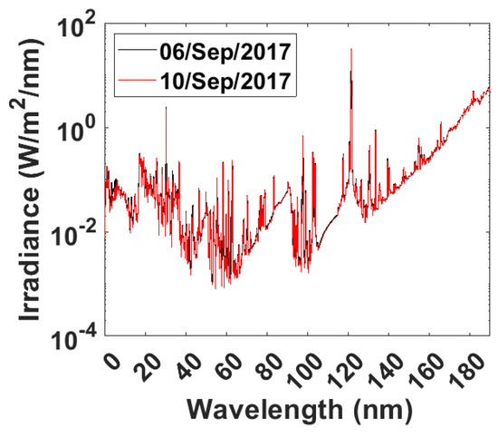
Figure 1.
FISM2 radiation data summed over 24 h for all wavelengths for flares on 6 September 2017 and 10 September 2017.
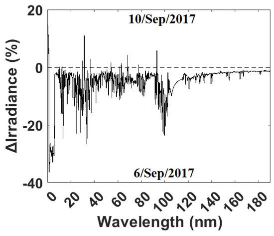
Figure 2.
Relative difference in radiation percentage of the outbreak on 10 September 2017 to 6 September 2017.
Thus, we can conclude that the X9.3 flare on 6 September was more powerful in the wavelength spectrum from 0 to 190 nm than the X8.2 flare on 10 September.
3. Model Description: HAMMONIA
In this paper, to analyze the changes in the chemistry and dynamics of the Earth’s atmosphere associated with solar flares in early September 2017, the HAMMONIA model [9] was used.
HAMMONIA was developed at MPI-M (Hamburg, Germany). HAMMONIA is a vertical extension of the MAECHAM5 model [11] to the middle thermosphere. HAMMONIA is a chemistry–climate model. It has horizontal resolution of about 2 × 2 degrees and 119 vertical levels covering the space from the ground to approximately 250 km. The model interactively treats dynamical, physical, and radiation processes and is coupled to the chemical module MOZART3. Dynamical and radiation processes include solar ultraviolet radiation, NONTLE scheme for the infrared radiation transfer, energy release and vortex diffusion, vertical molecular diffusion and conductivity, simplified parameterization of Joule heating and ion drag above the mesopause.
HAMMONIA helps to investigate how connections between atmospheric regions affect the response of the atmosphere to external disturbances, including variability in solar activity and anthropogenic chemical emissions at the Earth’s surface. HAMMONIA covers the troposphere, stratosphere and mesosphere, as well as a significant part of the thermosphere. Determining the penetration depth of the signal caused by the variability of solar activity in the atmosphere is a particularly difficult task. The solution to this problem requires that important chemical processes be considered fully interactive with the dynamic, physical, and radiation processes included in the model.
4. Description of HAMMONIA Model Experiments
In this paper, the HAMMONIA model used the FISM2 model data for 6 and 10 September for the entire spectrum from 0 to 190 nm as solar radiation. The wavelengths were divided into several intervals for each solar flare. One of the intervals of the spectrum starts from the shortest wavelengths and expands to 115 nm. The structure contains relatively narrow bands. The first band covers the range 29–32 nm, overlapping the He II line by 30.4 nm. Overlapping cells are also used in the ranges of 65.0–79.8 nm, 79.8–91.3, and 91.3–97.5 nm to obtain a realistic power distribution over the height. The boundaries of these ranges are determined by the ionization thresholds N, O, and O [12]. The other (119.9–188.7 nm) intervals of the spectrum are due to the formation of molecular oxygen (O) and nitric oxide (NO) in the ultraviolet wavelength range of atomic oxygen in the mesopause. First of all, photolysis of O and NO occurs in the Schumann–Runge continuum, Schumann–Runge bands, and at the Ly- wavelength. The wavelengths of the spectrum cover the location of the atmospheric window on the solar hydrogen line Ly- at a wavelength of 121.6 nm. The solar flux penetrates about 70 km, which can cause the photoionization of nitric oxide. In the continuation of the spectrum, absorption O is located in the region of the Schumann–Runge continuum (130–175 nm) and the Schumann–Runge bands (175–188.7 nm). The Schumann–Runge bands control attenuation in the mesosphere from about 65 to 90 km. The Schumann–Runge continuum becomes more important at about 90 km and above. This strong absorption is largely responsible for the transformation of O into an atomic form in the thermosphere. When absorbed in a continuum, oxygen atoms are in excited electronic states. The beginning of the continuum coincides with the energy required for the formation of an atom in the ground state and an atom in the first electronically excited state.
Using the HAMMONIA model, in September 2017, two numerical experiments with five ensemble members each were conducted to determine a statistically significant signal in the odd family of nitrogen (NO) and hydrogen (HO), as well as ozone, on the effect of solar electromagnetic radiation during flares on the sun. NO and hydrogen HO were chosen as the main ozone-depleting components of the atmosphere available for research using the HAMONNIA chemical climate model. The first numerical experiment was conducted taking into account the increase in radiation caused by solar flares on 6 and 10 September 2017, over the entire spectrum from 0 to 190 nm (). The second numerical experiment is a reference one; it does not take into account the processes associated with flare activity (). To assess the statistical significance of the results obtained, Student’s t-test was used.
5. Atmospheric Response
Figure 3 shows the response of the odd hydrogen group (HO) to the X9.3 flare on 6 September and X8.2 flare on 10 September 2017 (), with respect to the reference numerical experiment without solar flares () and results presented as (). Figure 3 shows that solar radiation during two solar flares on 6 and 10 September did not have a strong effect on the hydrogen group either in the northern polar latitudes, or in the equatorial latitudes, or in the southern latitudes. In the region of the southern polar latitudes (panel d), a slight increase in the odd hydrogen group by 3% is seen during two solar flares on 6 and 10 September. The HO signal from an increase in solar radiation is located locally and lasts for about several hours. The increase in the hydrogen group is noticeable within a few days of the outbreak in the mesosphere from about 10 to 1 Pa.
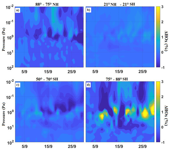
Figure 3.
The response of the hydrogen group HO (H, HO, HO) to solar flares X9.3 on 6 September and X8.2 on 10 September 2017 in the regions of northern polar latitudes (a), equatorial latitudes (b), southern latitudes (c), south polar latitudes (d).
Figure 4 is similar to Figure 3 only for the odd nitrogen family (NO). It can be seen from the analysis of the figure that solar radiation during two solar flares on 6 and 10 September led to an increase in the content of the odd nitrogen family in the northern polar and equatorial latitudes up to 40%. The effect is most pronounced in the mesosphere (from 10 to 1 Pa). It is important to note that the increase in NO after the X8.2 solar flare on 10 September exceeds the effect after the more powerful X9.3 flare on 6 September. Figure 4 shows that in the tropical mesosphere, the increase in NO is 40% after the flare on 10 September, which exceeds the increase in NO after the stronger (see Figure 2) flare on 6 September. This is because the X9.3 flare leads to an increase in NO of NO photolysis, followed by the reaction NO + N = N + O and a decrease in NO. Moreover, the signal from solar flares of the odd nitrogen family lasts for two weeks, which proves the long lifetime of NO.
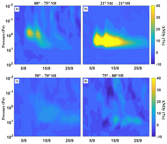
Figure 4.
The response of the odd nitrogen family NO (N, NO, NO, 2NO, HNO) to solar flares X9.3 on 6 September and X8.2 on 10 September 2017 in the northern polar latitudes (a), equatorial latitudes (b), southern latitudes (c), southern polar latitudes (d).
Figure 5 shows the ozone response to solar flares on 6 and 10 September. It can be seen from the figure that solar radiation did not affect the ozone content in the Earth’s atmosphere in any of the areas, except for a small peak in the southern high latitudes.
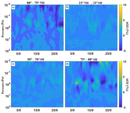
Figure 5.
The response of ozone (O) to solar flares X9.3 on 6 September and X8.2 on 10 September 2017 in the northern polar latitudes (a), equatorial latitudes (b), southern latitudes (c), and southern polar latitudes (d).
Thus, solar radiation after the X9.3 flares on 6 September and X8.2 on 10 September 2017 affected the increase in the hydrogen group by 3% in the southern polar latitudes and the increase in the odd nitrogen family by 40% in the northern, polar, and equatorial latitudes. However, at some points, we can identify some drops in ozone associated with rising HO. Significant changes in ozone concentrations in the composition of the Earth’s atmosphere after solar flares were not observed.
6. Conclusions
In this paper, we studied the effect of solar flare activity in September 2017 on the ozone-depleting components and the ozone layer in the Earth’s atmosphere. For this, the two largest class X solar flares of the 24th solar cycle, the X9.3 flare on 6 September and the X8.2 flare on 10 September 2017, were selected.
Data on radiation fluxes over the entire wavelength spectrum from 0 to 190 nm from solar flares in early September 2017 were obtained using the FISM2 empirical model.
Using the HAMMONIA chemistry–climate model, two numerical ensemble experiments with five realizations were performed to determine a statistically significant signal. The odd nitrogen family (NO) and the odd hydrogen group (HO) were chosen as the main ozone-depleting components of the atmosphere. The first numerical experiment was conducted considering solar flares on 6 and 10 September 2017 over the entire spectrum from 0 to 190 nm. The second numerical experiment, which was a reference one, was conducted without flares. Between model simulations, statistical significance was calculated for the reliability of the results obtained.
It was shown that the hydrogen group (HO) is only marginally affected by flare activity over the equatorial and northern polar latitudes. In the southern polar latitudes, a slight increase in HO was obtained. Analyzing the response of the odd nitrogen family, it was shown that solar radiation during two solar flares on 6 and 10 September 2017 enhanced the NO concentration by up to 40% in the mesosphere at a level of about 1 Pa in the regions of northern polar and equatorial latitudes. It is interesting that over the northern high latitudes, the weaker X8.2 flare on 10 September resulted in a less pronounced increase in NO, while in the tropical mesosphere, the responses are different and the increase in NO after the 10 September flare exceeds the effect of the more powerful flare on 6 September. This phenomenon is explained by the different NO response to the enhancement of the solar irradiance at different wavelengths. The increase of the shortwave (below 180 nm) solar irradiance intensifies NO production, while the increase of solar irradiance in the Schumann–Runge bands (180–200 nm) contributes to the destruction of NO due to NO photolysis, followed by the NO + N = N + O reaction.
It is important to note that solar flares in early September 2017 led to a significant increase in the concentrations of the reactive nitrogen and hydrogen oxides in the equatorial latitudes and southern high latitudes. However, this increase did not affect the change in the ozone content in the tropical stratosphere because the ozone destruction by nitrogen oxides is not effective in the upper mesosphere and there are no persistent downward motions, which can transport extra NO down to the stratosphere. Hydrogen oxides do not have major influence on the ozone during the considered seasons, however, some small ozone depletion correlated with HO increase is simulated in the southern hemisphere.
Thus, we can conclude that the ozone changes caused by processes that are associated with the impact of electromagnetic radiation on the Earth’s atmosphere during solar flares are not dramatic.
Author Contributions
I.M. and E.R. discussed the manuscript’s idea; P.P. and E.R. worked with FISM2 data under the Project RSF 20-67-46016; I.M., A.K. and P.P. worked on HAMMONIA model data treatment and visualization under the Project RSF 20-67-46016. All authors discussed the results and commented on the manuscript. All authors have read and agreed to the published version of the manuscript.
Funding
The work of P.P., I.M., E.R. and A.K. was supported by a grant from the Russian Science Foundation (Project RSF 20-67-46016). This work was carried out at “Laboratory for the study of the ozone layer and the upper atmosphere” with the support of the Ministry of Science and Higher Education of the Russian Federation under agreement 075-15-2021-583.
Data Availability Statement
All data can be provided upon request.
Acknowledgments
The acknowledgment to Timofei Sukhodolov for HAMMONIA model simulation.
Conflicts of Interest
The authors declare no conflict of interest.
References
- Farman, J.C.; Gardiner, B.G.; Shanklin, J.D. Large losses of total ozone in Antarctica reveal seasonal ClOx/NOx interaction. Nature 1985, 315, 207–210. [Google Scholar] [CrossRef]
- Dobson, G. Exploring the Atmosphere; Oxford University Press: Oxford, UK, 1968. [Google Scholar]
- Brasseur, G.P.; Solomon, S.C. Aeronomy of the Middle Atmosphere; Springer Science & Business Media: Berlin, Germany, 2009. [Google Scholar]
- Rozanov, E.; Calisto, M.; Egorova, T.; Peter, T.; Schmutz, W. Influence of the Precipitating Energetic Particles on Atmospheric Chemistry and Climate. Surv. Geophys. 2012, 33, 483–501. [Google Scholar] [CrossRef] [Green Version]
- Ball, W.T.; Rozanov, E.V.; Alsing, J.; Marsh, D.R.; Tummon, F.; Mortlock, D.J.; Kinnison, D.; Haigh, J.D. The Upper Stratospheric Solar Cycle Ozone Response. Geophys. Res. Lett. 2019, 46, 1831–1841. [Google Scholar] [CrossRef] [Green Version]
- Mironova, I.; Karagodin-Doyennel, A.; Rozanov, E. The effect of Forbush decreases on the polar-night HOx concentration affecting stratospheric ozone. Front. Earth Sci. 2021, 8, 669. [Google Scholar] [CrossRef]
- Schmidt, H.; Brasseur, G.P. The Response of the Middle Atmosphere to Solar Cycle Forcing in the Hamburg Model of the Neutral and Ionized Atmosphere. Space Sci. Rev. 2006, 125, 345–356. [Google Scholar] [CrossRef]
- Minschwaner, K.; Siskind, D.E. A new calculation of nitric oxide photolysis in the stratosphere, mesosphere, and lower thermosphere. J. Geophys. Res. 1993, 98, 20401–20412. [Google Scholar] [CrossRef]
- Schmidt, H.; Brasseur, G.P.; Charron, M.; Manzini, E.; Giorgetta, M.A.; Diehl, T.; Fomichev, V.I.; Kinnison, D.; Marsh, D.; Walters, S. The HAMMONIA Chemistry Climate Model: Sensitivity of the Mesopause Region to the 11-Year Solar Cycle and CO2 Doubling. J. Clim. 2006, 19, 3903. [Google Scholar] [CrossRef] [Green Version]
- Chamberlin, P.C.; Woods, T.N.; Eparvier, F.G. Flare Irradiance Spectral Model (FISM): Flare component algorithms and results. Space Weather 2008, 6, S05001. [Google Scholar] [CrossRef]
- Giorgetta, M.A.; Manzini, E.; Roeckner, E.; Esch, M.; Bengtsson, L. Climatology and Forcing of the Quasi-Biennial Oscillation in the MAECHAM5 Model. J. Clim. 2006, 19, 3882. [Google Scholar] [CrossRef] [Green Version]
- Solomon, S.C.; Qian, L. Solar extreme-ultraviolet irradiance for general circulation models. J. Geophys. Res. 2005, 110, A10306. [Google Scholar] [CrossRef] [Green Version]
Publisher’s Note: MDPI stays neutral with regard to jurisdictional claims in published maps and institutional affiliations. |
© 2022 by the authors. Licensee MDPI, Basel, Switzerland. This article is an open access article distributed under the terms and conditions of the Creative Commons Attribution (CC BY) license (https://creativecommons.org/licenses/by/4.0/).