
An Integrated Change Detection Method Based on Spectral Unmixing and the CNN for Hyperspectral Imagery


Abstract
:
1. Introduction
2. Related Works
2.1. Spectral Unmixing
2.2. Machine Learning
2.3. Deep Learning
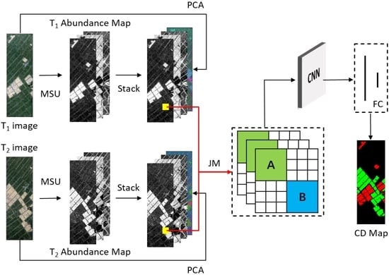
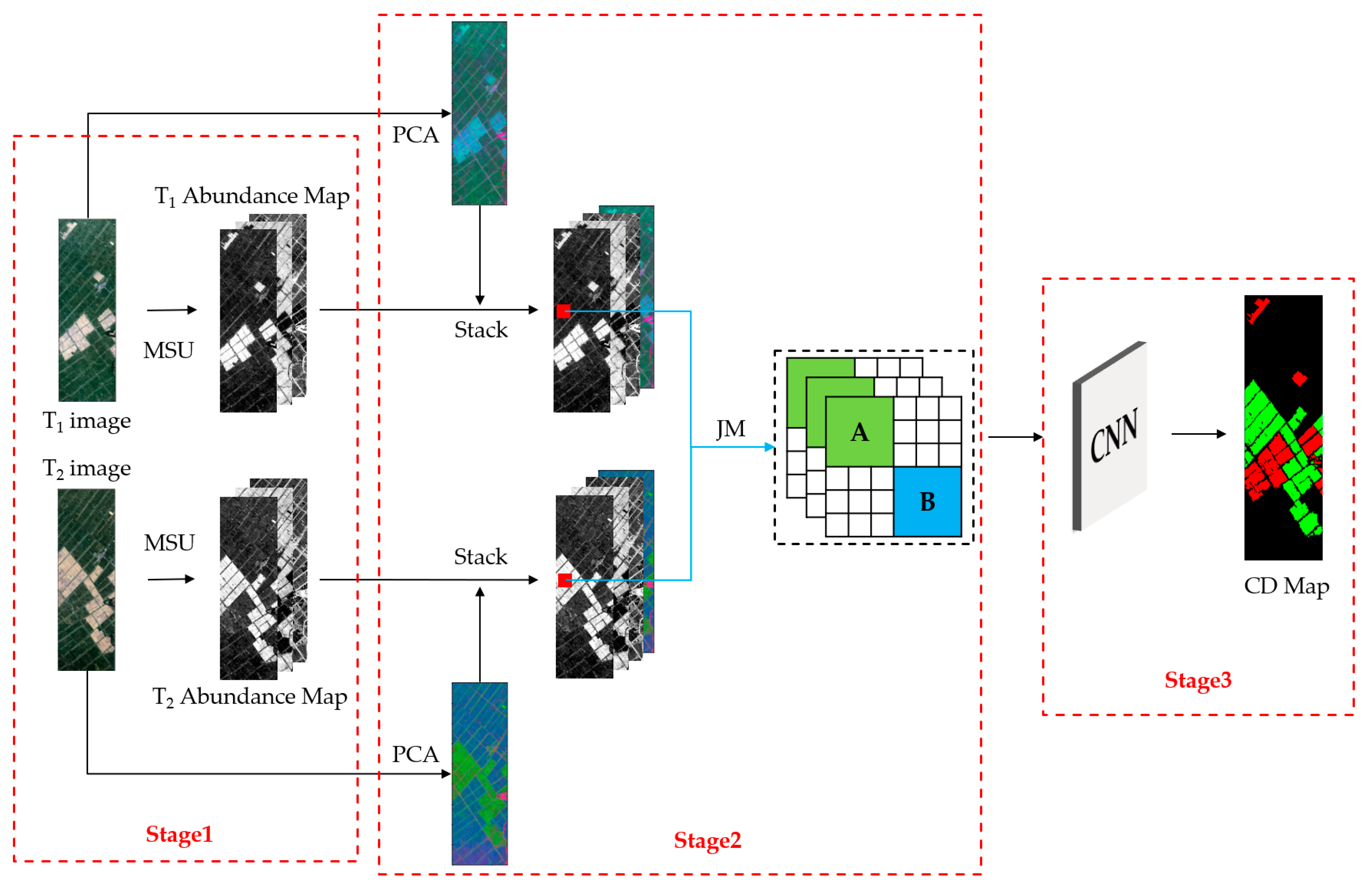
3. Methodology
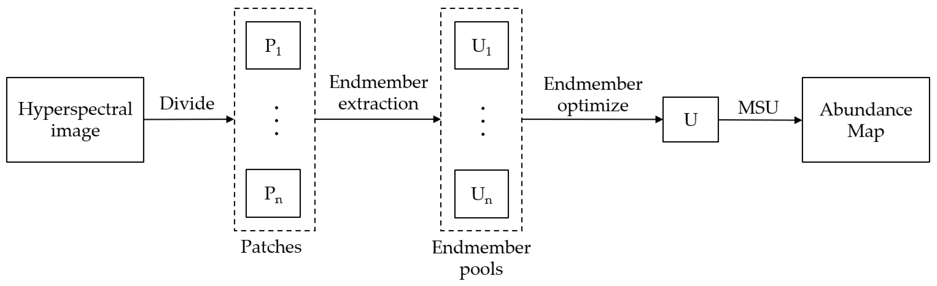
3.1. MSU Method for Acquiring Abundance Images
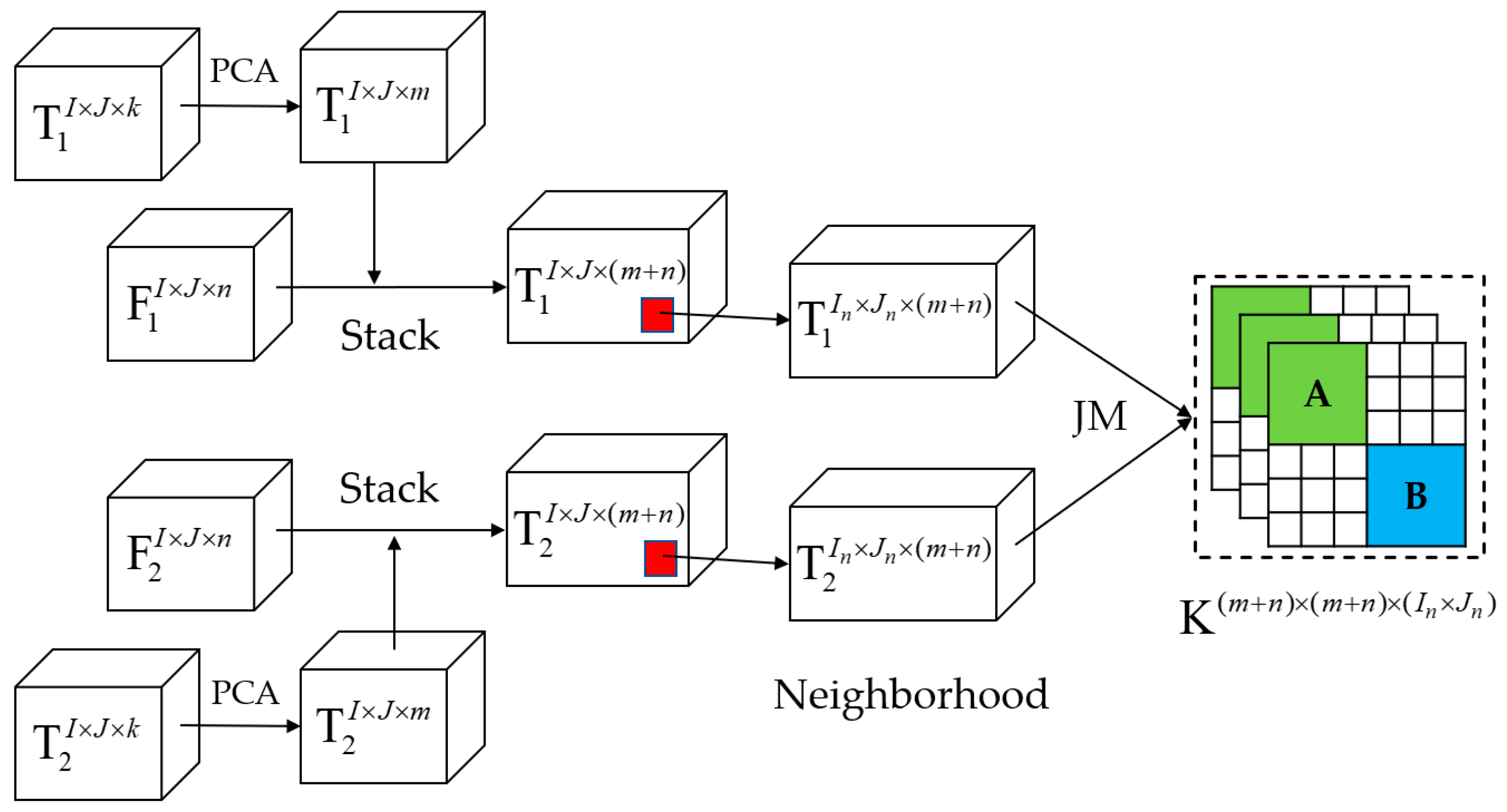
3.2. JM Algorithm for Information Fusion
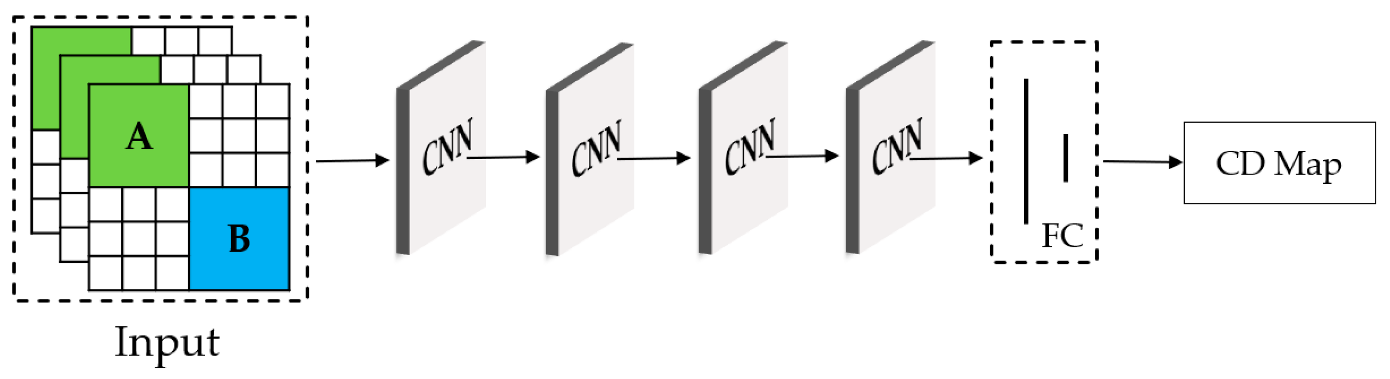
3.3. CNN for Detecting Multiple Changes
4. Experiment
4.1. Dataset Description
4.2. Evaluation Measures
4.3. Results and Discussion
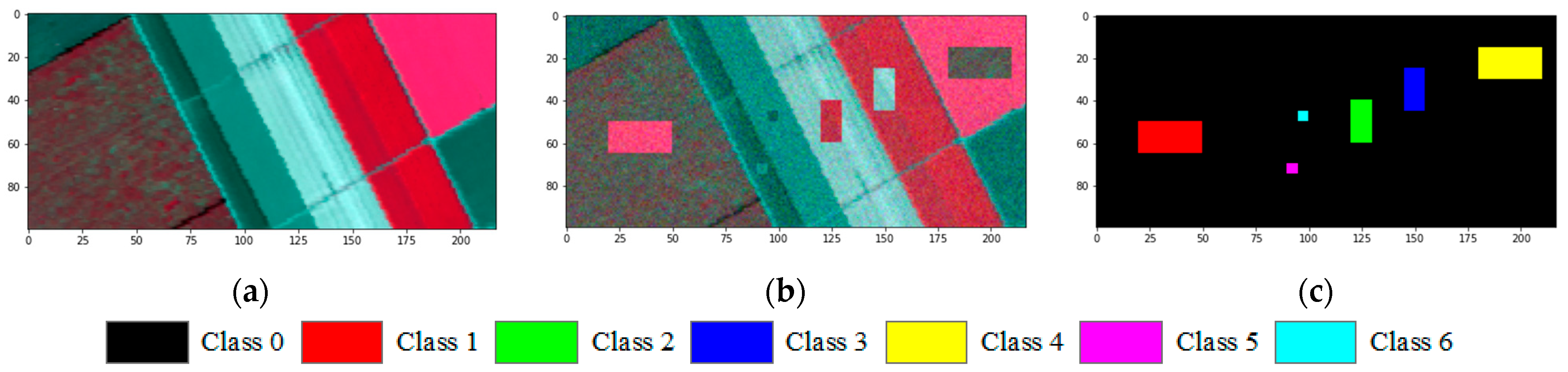
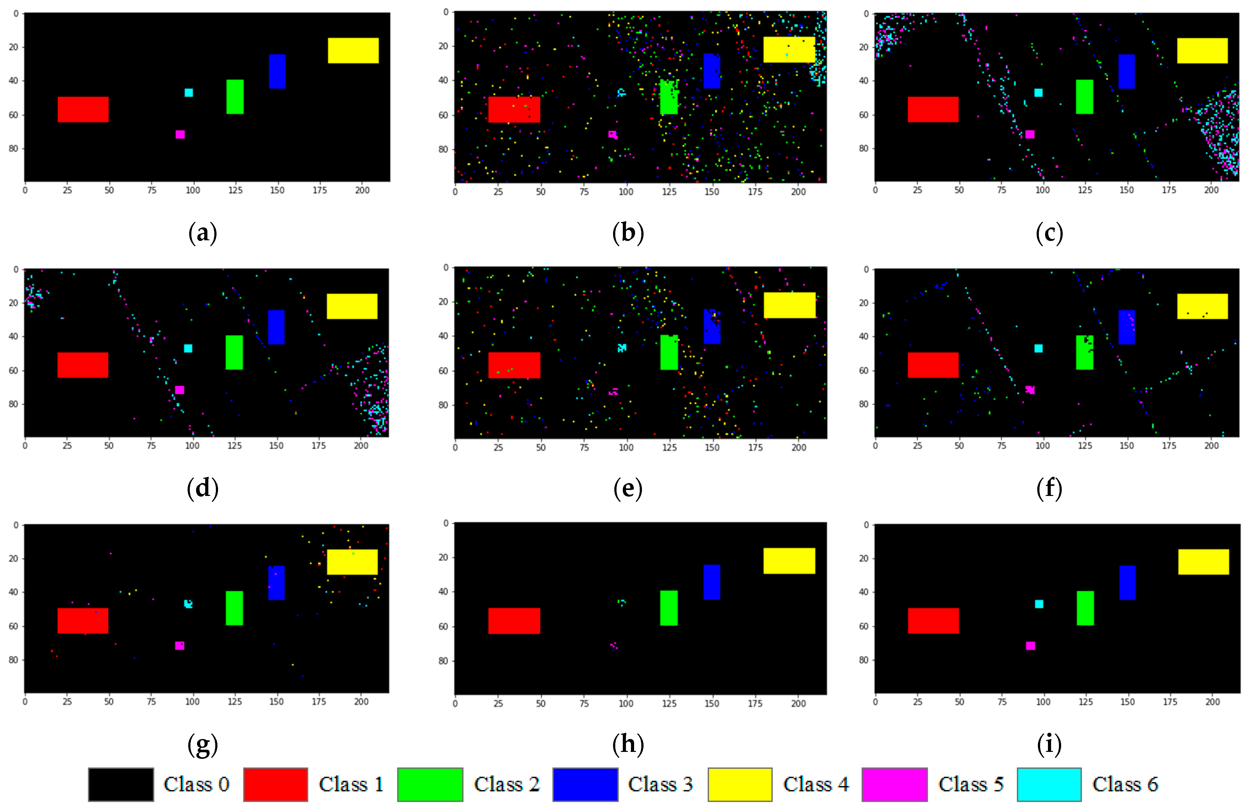
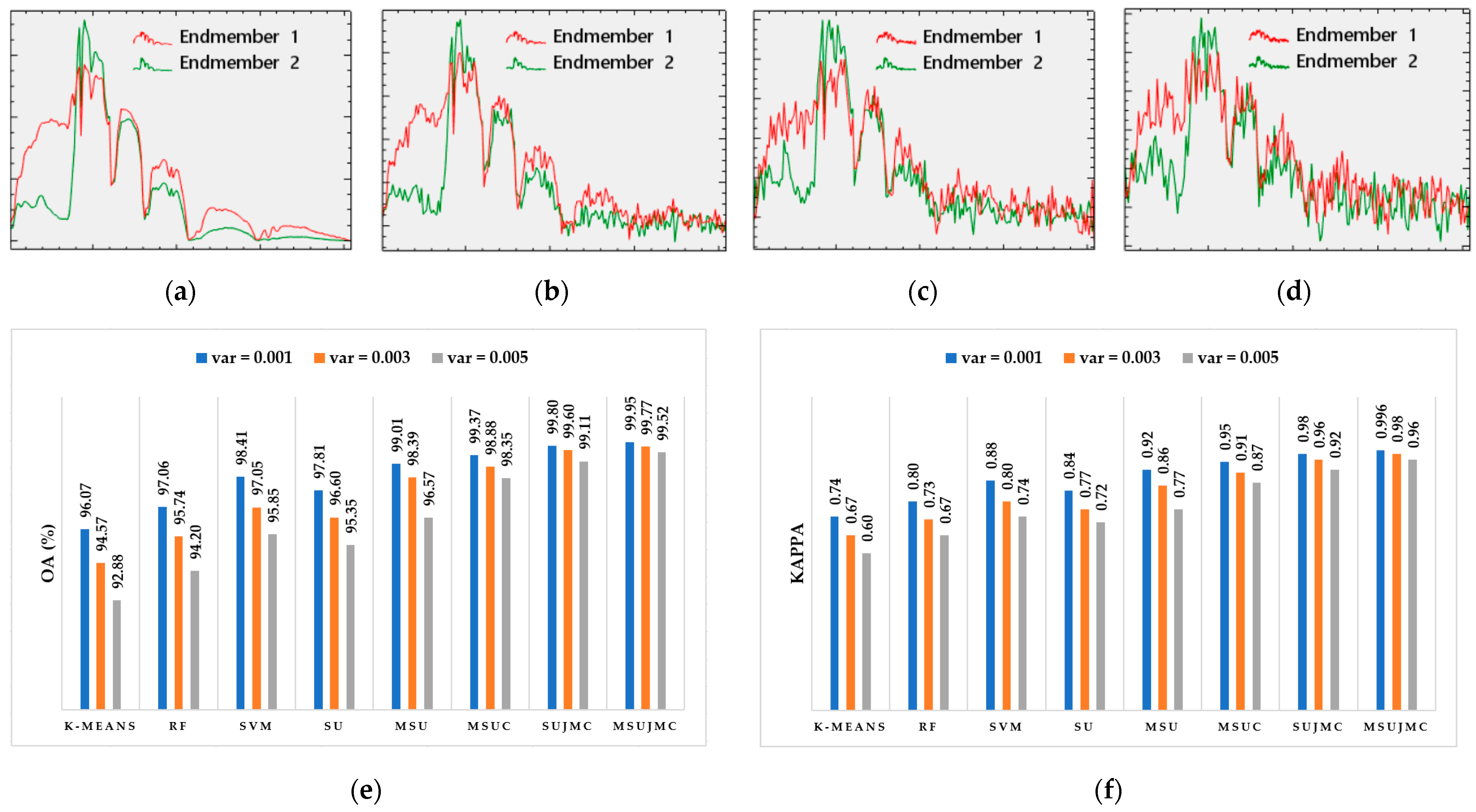
4.3.1. Simulation Dataset
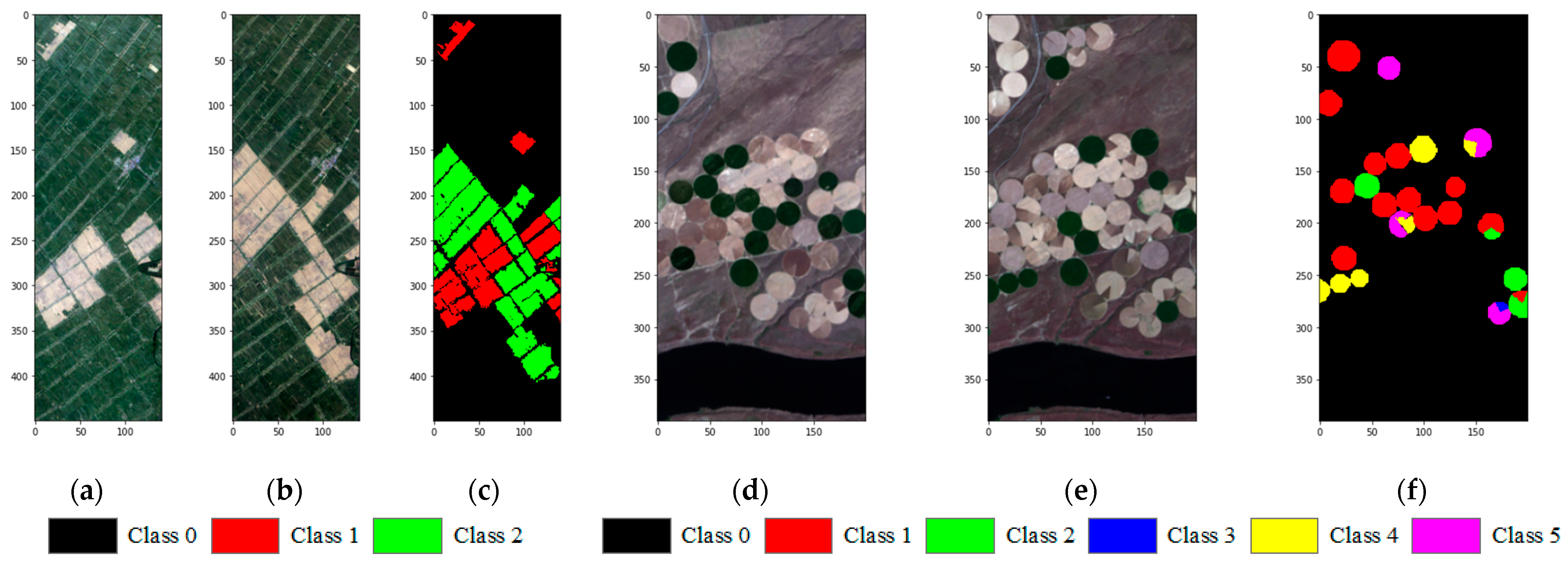
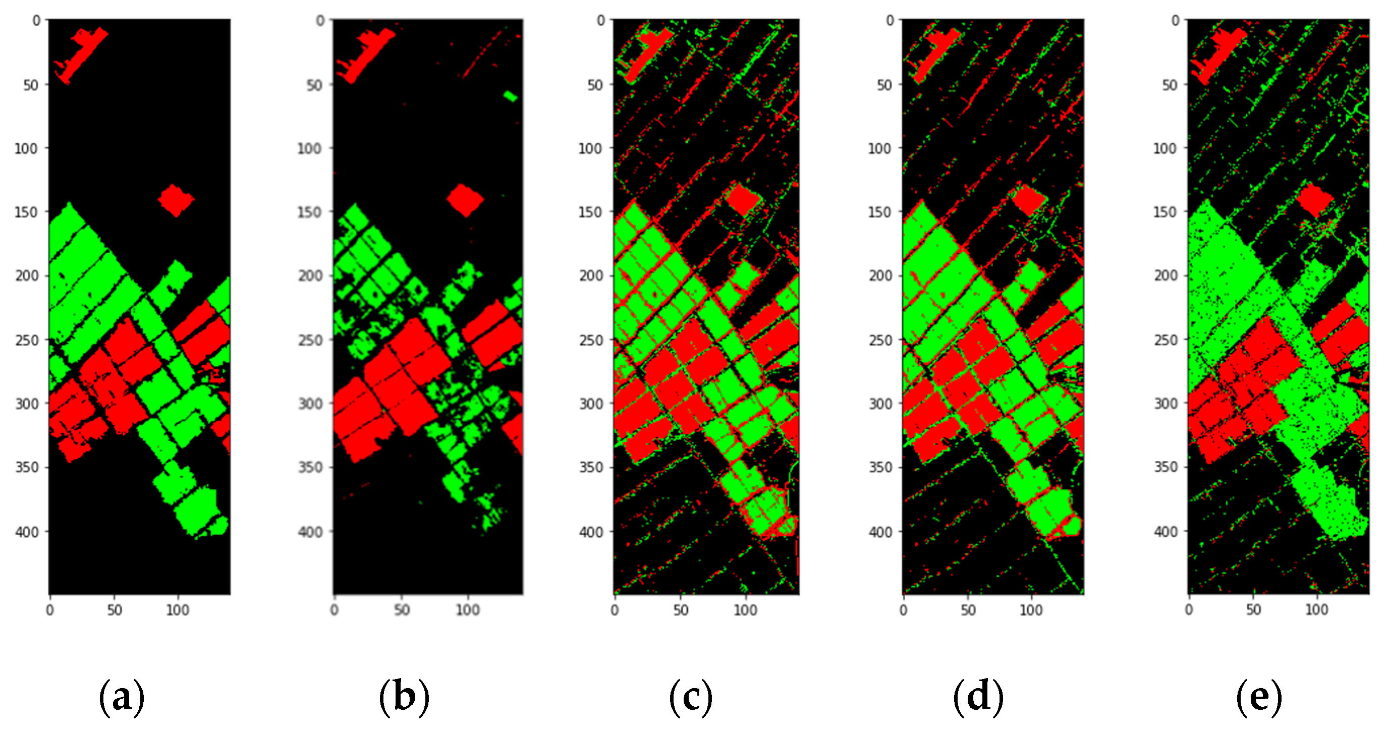
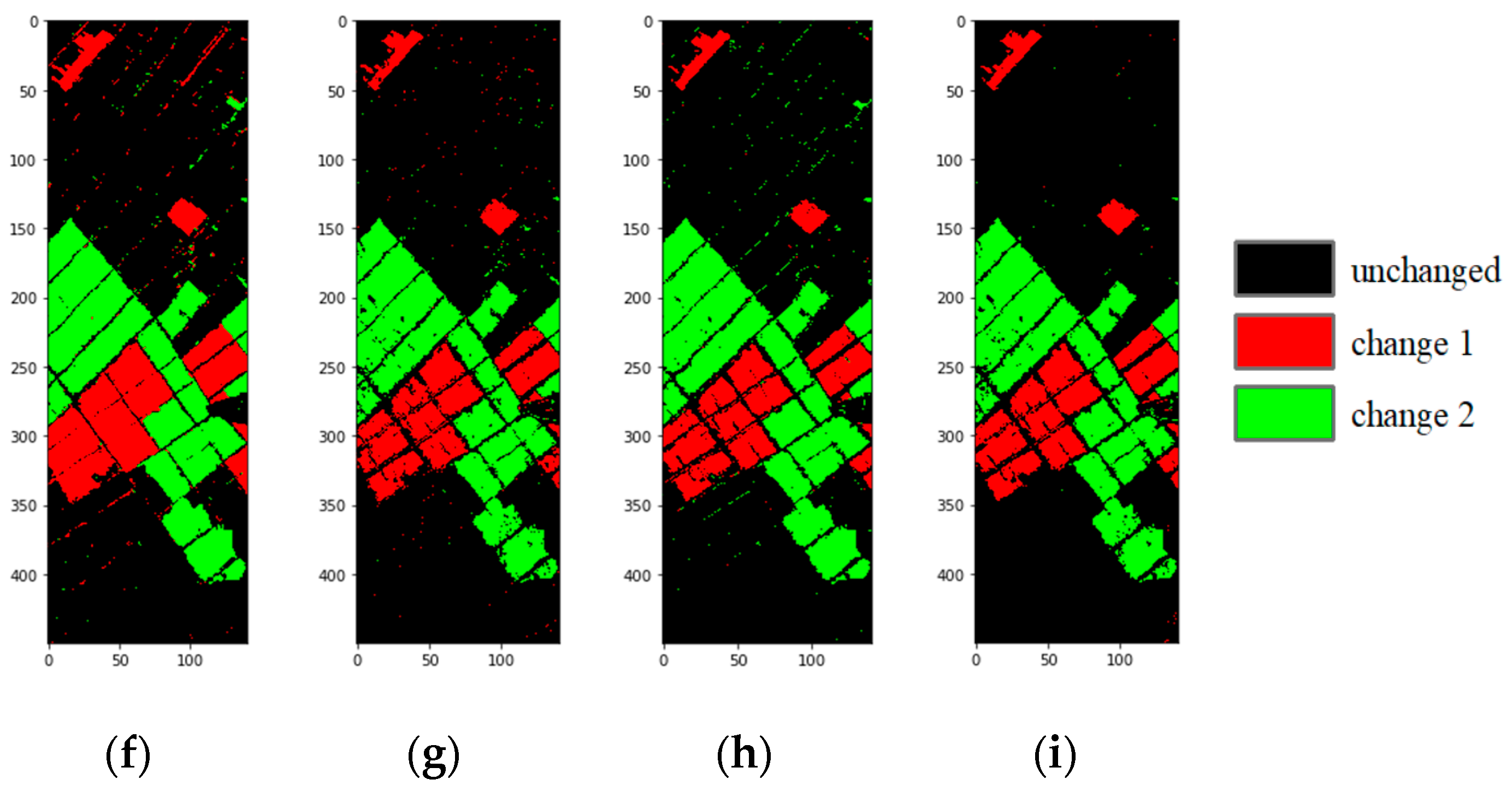
4.3.2. Real HSI Dataset-1
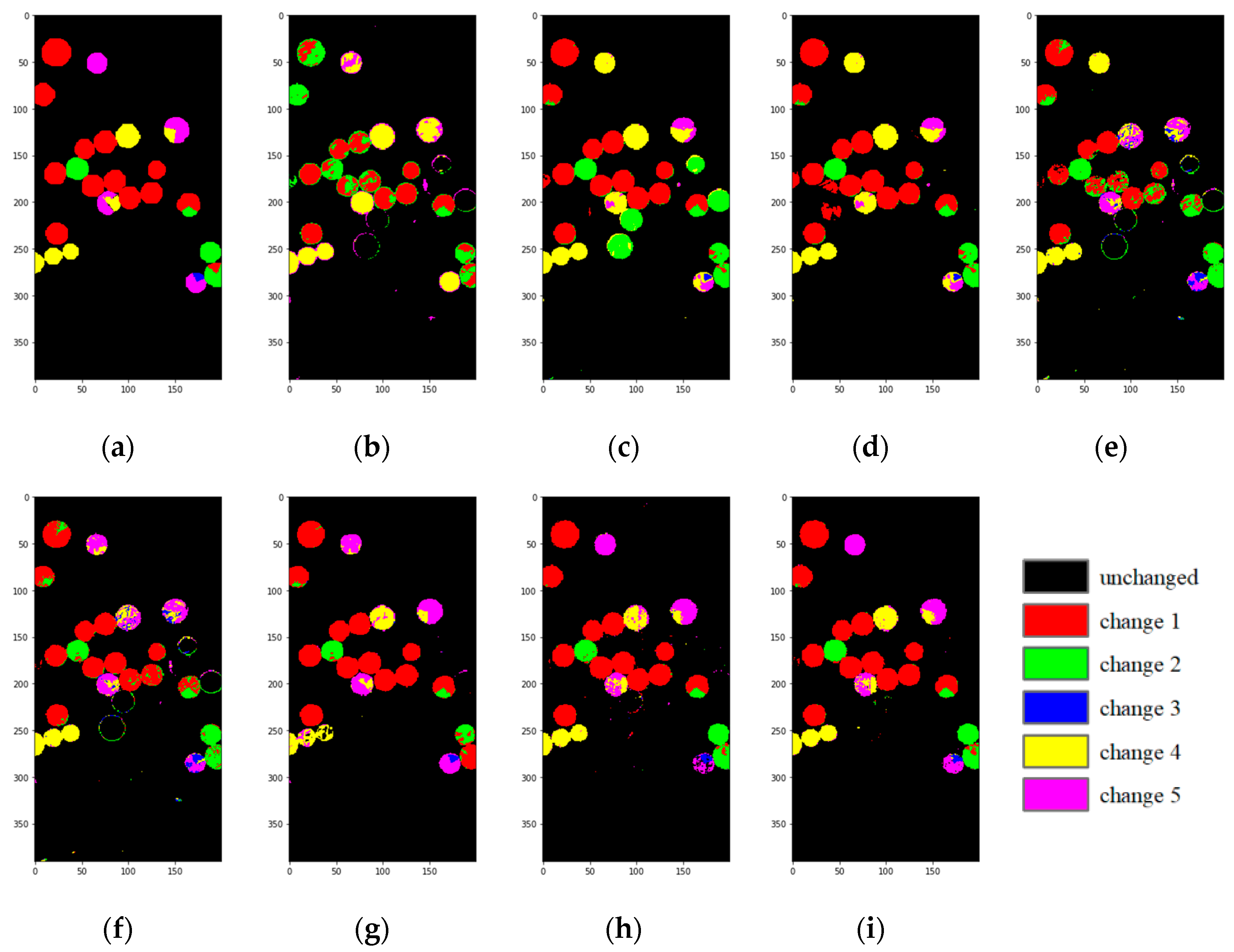
4.3.3. Real HSI Dataset-2
4.4. Computational Cost Analysis
5. Conclusions
Author Contributions
Funding
Data Availability Statement
Acknowledgments
Conflicts of Interest
References
- Asokan, A.; Anitha, J. Change detection techniques for remote sensing applications: A survey. Earth Sci. Inform. 2019, 12, 143–160. [Google Scholar] [CrossRef]
- Zhang, L.; Wu, C. Advance and Future Development of Change Detection for Multi-temporal Remote Sensing Imagery. Acta Geod. Cartogr. Sin. 2017, 46, 1447. [Google Scholar]
- Liu, W.; Xu, J.; Guo, Z.; Li, E.; Li, X.; Zhang, L.; Liu, W. Building Footprint Extraction from Unmanned Aerial Vehicle Images Via PRU-Net: Application to Change Detection. IEEE J. Sel. Top. Appl. Earth Obs. Remote Sens. 2021, 14, 2236–2248. [Google Scholar] [CrossRef]
- Kaliraj, S.; Meenakshi, S.M.; Malar, V.K. Application of Remote Sensing in Detection of Forest Cover Changes Using Geo-Statistical Change Detection Matrices—A Case Study of Devanampatti Reserve Forest, Tamilnadu, India Nature Environment and Pollution Technology. Nat. Environ. Pollut. Technol. 2012, 11, 261–269. [Google Scholar]
- Zhang, Q.; Yang, N.; Li, X. Application and Future Development of Land Use Change Detection Based on Remote Sensing Technology in China. In Proceedings of the 2010 Asia-Pacific Conference on Power Electronics and Design, Wuhan, China, 30–31 May 2010. [Google Scholar]
- Benedetti, A.; Picchiani, M.; Frate, F.D. Sentinel-1 and Sentinel-2 Data Fusion for Urban Change Detection. In Proceedings of the IGARSS 2018—2018 IEEE International Geoscience and Remote Sensing Symposium, Valencia, Spain, 22–27 July 2018. [Google Scholar]
- Usha, S.G.A.; Vasuki, S. Unsupervised Change Detection of Multispectral Imagery Using Multi Level Fuzzy Based Deep Representation. J. Asian Sci. Res. 2017, 7, 206–213. [Google Scholar] [CrossRef] [Green Version]
- Bruzzone, L.; Bovolo, F. A Novel Framework for the Design of Change-Detection Systems for Very-High-Resolution Remote Sensing Images. Proc. IEEE 2013, 101, 609–630. [Google Scholar] [CrossRef]
- Tewkesbury, A.P.; Comber, A.J.; Tate, N.J.; Lamb, A.; Fisher, P.F. A critical synthesis of remotely sensed optical image change detection techniques. Remote Sens. Environ. 2015, 160, 1–14. [Google Scholar] [CrossRef] [Green Version]
- Erturk, A.; Iordache, M.D.; Plaza, A. Sparse Unmixing with Dictionary Pruning for Hyperspectral Change Detection. IEEE J. Sel. Top. Appl. Earth Obs. Remote Sens. 2017, 10, 321–330. [Google Scholar] [CrossRef]
- Liu, S.; Bruzzone, L.; Bovolo, F.; Du, P. A novel hierarchical method for change detection in multitemporal hyperspectral images. In Proceedings of the IEEE International Geoscience & Remote Sensing Symposium, Melbourne, Australia, 21–26 July 2013. [Google Scholar]
- Wu, C.; Du, B.; Zhang, L. A Subspace-Based Change Detection Method for Hyperspectral Images. IEEE J. Sel. Top. Appl. Earth Obs. Remote Sens. 2013, 6, 815–830. [Google Scholar] [CrossRef]
- Seydi, S.T.; Shah-Hosseini, R.; Hasanlou, M. New framework for hyperspectral change detection based on multi-level spectral unmixing. Appl. Geomat. 2021, 13, 763–780. [Google Scholar] [CrossRef]
- Ruggeri, S.; Henao-Cespedes, V.; Garcés-Gómez, Y.A.; Uzcátegui, A.P. Optimized unsupervised CORINE Land Cover mapping using linear spectral mixture analysis and object-based image analysis—ScienceDirect. Egypt. J. Remote Sens. Space Sci. 2021, 24, 1061–1069. [Google Scholar]
- Haertel, V.; Shimabukuro, Y.E.; Almeida-Filho, R. Fraction images in multitemporal change detection. Int. J. Remote Sens. 2004, 25, 5473–5489. [Google Scholar] [CrossRef]
- Wu, K.; Du, Q.; Wang, Y.; Yang, Y. Supervised Sub-Pixel Mapping for Change Detection from Remotely Sensed Images with Different Resolutions. Remote Sens. 2017, 9, 284. [Google Scholar] [CrossRef] [Green Version]
- Keshava, N.; Mustard, J.F. Spectral unmixing. IEEE Signal Process. Mag. 2002, 19, 44–57. [Google Scholar] [CrossRef]
- Afarzadeh, H.J.; Hasanlou, M. An Unsupervised Binary and Multiple Change Detection Approach for Hyperspectral Imagery Based on Spectral Unmixing. IEEE J. Sel. Top. Appl. Earth Obs. Remote Sens. 2020, 12, 4888–4906. [Google Scholar] [CrossRef]
- Erturk, A.; Iordache, M.D.; Plaza, A. Sparse Unmixing-Based Change Detection for Multitemporal Hyperspectral Image. IEEE J. Sel. Top. Appl. Earth Obs. Remote Sens. 2017, 9, 708–719. [Google Scholar] [CrossRef]
- Erturk, A.; Plaza, A. Informative Change Detection by Unmixing for Hyperspectral Images. IEEE Geosci. Remote Sens. Lett. 2017, 12, 1252–1256. [Google Scholar] [CrossRef]
- Wu, K.; Du, Q. Subpixel Change Detection of Multitemporal Remote Sensed Images Using Variability of Endmembers. IEEE Geosci. Remote Sens. Lett. 2017, 14, 796–800. [Google Scholar] [CrossRef]
- Liu, S.; Bruzzone, L.; Bovolo, F.; Du, P. Hierarchical Unsupervised Change Detection in Multitemporal Hyperspectral Images. IEEE Trans. Geosci. Remote Sens. 2014, 53, 244–260. [Google Scholar]
- Wu, K.; Chen, T.; Xu, Y.; Song, D.; Li, H. A Novel Change Detection Approach Based on Spectral Unmixing from Stacked Multitemporal Remote Sensing Images with a Variability of Endmembers. Remote Sens. 2021, 13, 2550. [Google Scholar] [CrossRef]
- Hong, D.; Yokoya, N.; Chanussot, J.; Zhu, X.X. An Augmented Linear Mixing Model to Address Spectral Variability for Hyperspectral Unmixing. IEEE Trans. Image Process. 2018, 28, 1923–1938. [Google Scholar] [CrossRef] [PubMed] [Green Version]
- Wong, R.S.; Ford, G.E.; Paglieroni, D.W. K-means reclustering: An alternative approach to automatic target cueing in hyperspectral images. Proc. SPIE 2002, 4726, 162–172. [Google Scholar]
- Bovolo, F.; Bruzzone, L. A Theoretical Framework for Unsupervised Change Detection Based on Change Vector Analysis in the Polar Domain. IEEE Trans. Geosci. Remote Sens. 2006, 45, 218–236. [Google Scholar] [CrossRef] [Green Version]
- Botsch, M.; Nossek, J.A. Feature Selection for Change Detection in Multivariate Time-Series. In Proceedings of the IEEE Symposium on Computational Intelligence & Data Mining, Honolulu, HI, USA, 1 March–5 April 2007. [Google Scholar]
- Gapper, J.J.; El-Askary, H.; Linstead, E.; Piechota, T. Coral Reef Change Detection in Remote Pacific Islands Using Support Vector Machine Classifiers. Remote Sens. 2019, 11, 1525. [Google Scholar] [CrossRef] [Green Version]
- Zong, K.; Sowmya, A.; Trinder, J. Building change detection from remotely sensed images based on spatial domain analysis and Markov random field. J. Appl. Remote Sens. 2019, 13, 024514. [Google Scholar] [CrossRef]
- Im, J.; Jensen, J.R. A change detection model based on neighborhood correlation image analysis and decision tree classification. Remote Sens. Environ. 2005, 99, 326–340. [Google Scholar] [CrossRef]
- Pu, R.; Gong, P.; Tian, Y.; Miao, X.; Carruthers, R.I.; Anderson, G.L. Invasive species change detection using artificial neural networks and CASI hyperspectral imagery. Environ. Monit. Assess. 2008, 140, 15. [Google Scholar] [CrossRef]
- Hussein, G.A. Retrospective change detection for binary time series models. J. Stat. Plan. Inference 2014, 145, 102–112. [Google Scholar]
- Zhan, T.; Song, B.; Sun, L.; Jia, X.; Wan, M.; Yang, G.; Wu, Z. TDSSC: A Three-Directions Spectral–Spatial Convolution Neural Network for Hyperspectral Image Change Detection. IEEE J. Sel. Top. Appl. Earth Obs. Remote Sens. 2020, 14, 377–388. [Google Scholar] [CrossRef]
- Huang, F.; Yu, Y.; Feng, T. Hyperspectral remote sensing image change detection based on tensor and deep learning. J. Vis. Commun. Image Represent. 2019, 58, 233–244. [Google Scholar] [CrossRef]
- Seydi, S.T.; Hasanlou, M. Binary hyperspectral change detection based on 3D convolution deep learning. Int. Arch. Photogramm. Remote Sens. Spat. Inf. Sci. 2020, 43, 1–5. [Google Scholar] [CrossRef]
- Nascimento, J.; Dias, J. Vertex component analysis: A fast algorithm to unmix hyperspectral data. IEEE Trans. Geosci. Remote Sens. 2005, 43, 898–910. [Google Scholar] [CrossRef] [Green Version]
- Garcia-Allende, P.B.; Conde, O.M.; Mirapeix, J.; Cubillas, A.M.; Lopez-Higuera, J.M. Data Processing Method Applying Principal Component Analysis and Spectral Angle Mapper for Imaging Spectroscopic Sensors. IEEE Sens. J. 2008, 8, 1310–1316. [Google Scholar] [CrossRef]
- Quintano, C.; Fernández-Manso, A.; Roberts, D.A. Multiple Endmember Spectral Mixture Analysis (MESMA) to map burn severity levels from Landsat images in Mediterranean countries. Remote Sens. Environ. 2013, 136, 76–88. [Google Scholar] [CrossRef]
- Du, Q.; Wasson, L.; King, R. Unsupervised linear unmixing for change detection in multitemporal airborne hyperspectral imagery. In International Workshop on the Analysis of Multi-Temporal Remote Sensing Images; IEEE: Piscataway, NJ, USA, 2005. [Google Scholar]
- Foody, G.M.; Cox, D.P. Sub-pixel land cover composition estimation using a linear mixture model and fuzzy membership functions. Int. J. Remote Sens. 1994, 15, 619–631. [Google Scholar] [CrossRef]
- Heinz, D.C. Fully constrained least squares linear spectral mixture analysis method for material quantification in hyperspectral imagery. IEEE Trans. Geosci. Remote Sens. 2002, 39, 529–545. [Google Scholar] [CrossRef] [Green Version]
- Liu, Y.; Zhang, Q.; Chen, Y.; Cheng, Q.; Peng, C. Hyperspectral Image Denoising with Log-Based Robust PCA. In Proceedings of the 2021 IEEE International Conference on Image Processing (ICIP), Anchorage, AK, USA, 19–22 September 2021. [Google Scholar]
- Dong, Y.; Liu, Q.; Du, B.; Zhang, L. Weighted Feature Fusion of Convolutional Neural Network and Graph Attention Network for Hyperspectral Image Classification. IEEE Trans. Image Process. 2022, 31, 1559–1572. [Google Scholar] [CrossRef]
- Han, J.; Kang, D.S. CoS: An Emphasized Smooth Non-Monotonic Activation Function Consisting of Sigmoid for Deep Learning. J. Korean Inst. Inform. Technol. 2021, 19, 1–9. [Google Scholar]
- Liu, X.; Di, X. TanhExp: A Smooth Activation Function with High Convergence Speed for Lightweight Neural Networks. IET Comput. Vis. 2020, 15, 136–150. [Google Scholar] [CrossRef]
- Hao, X.; Zhang, G.; Ma, S. Deep Learning. Int. J. Semant. Comput. 2016, 10, 417–439. [Google Scholar] [CrossRef] [Green Version]
- Alhassan, A.M.; Wan, M. Brain tumor classification in magnetic resonance image using hard swish-based RELU activation function-convolutional neural network. Neural Comput. Appl. 2021, 33, 9075–9087. [Google Scholar] [CrossRef]

| Layers | Type | Channels | Kernel Size |
|---|---|---|---|
| Conv1 | Convolution + BN Activation (relu) | 16 | 3 × 3 |
| Pool1 | MaxPooling | - | 2 × 2 |
| Conv2 | Convolution + BN Activation (relu) | 32 | 3 × 3 |
| Pool2 | MaxPooling | - | 2 × 2 |
| Conv3 | Convolution + BN Activation (relu) | 64 | 3 × 3 |
| Pool3 | MaxPooling | - | 2 × 2 |
| Conv4 | Convolution + BN Activation (relu) | 128 | 3 × 3 |
| Pool4 | MaxPooling | - | 2 × 2 |
| FC1 | Fully Connected + BN Activation (relu) | 128 | - |
| FC2 | Fully Connected + BN Activation (softmax) | nchange + 1 | - |
| K-means | RF | SVM | SU | MSU | MSUC | SUJMC | MSUJMC | ||
|---|---|---|---|---|---|---|---|---|---|
| OA (%) | 96.07 | 97.06 | 98.41 | 97.81 | 99.01 | 99.37 | 99.80 | 99.95 | |
| Kappa | 0.74 | 0.80 | 0.88 | 0.84 | 0.92 | 0.95 | 0.98 | 0.996 | |
| unchanged | Precision | 1.00 | 1.00 | 1.00 | 1.00 | 1.00 | 1.00 | 1.00 | 1.00 |
| Recall | 0.96 | 0.97 | 0.98 | 0.98 | 0.99 | 0.99 | 1.00 | 1.00 | |
| change 1 | Precision | 0.80 | 1.00 | 1.00 | 0.86 | 1.00 | 0.95 | 1.00 | 1.00 |
| Recall | 0.99 | 1.00 | 1.00 | 0.99 | 1.00 | 1.00 | 1.00 | 1.00 | |
| change 2 | Precision | 0.48 | 0.80 | 0.91 | 0.68 | 0.80 | 1.00 | 0.99 | 1.00 |
| Recall | 0.91 | 1.00 | 1.00 | 0.98 | 0.95 | 1.00 | 1.00 | 1.00 | |
| change 3 | Precision | 0.54 | 0.80 | 0.88 | 0.66 | 0.72 | 0.95 | 1.00 | 1.00 |
| Recall | 0.96 | 1.00 | 1.00 | 0.82 | 0.97 | 0.97 | 1.00 | 1.00 | |
| change 4 | Precision | 0.75 | 1.00 | 1.00 | 0.82 | 1.00 | 0.95 | 1.00 | 1.00 |
| Recall | 0.99 | 1.00 | 1.00 | 1.00 | 0.99 | 1.00 | 1.00 | 1.00 | |
| change 5 | Precision | 0.21 | 0.10 | 0.17 | 0.23 | 0.41 | 0.76 | 1.00 | 1.00 |
| Recall | 0.72 | 1.00 | 1.00 | 0.40 | 0.84 | 0.95 | 0.16 | 0.84 | |
| change 6 | Precision | 0.09 | 0.07 | 0.13 | 0.32 | 0.36 | 0.72 | 1.00 | 1.00 |
| Recall | 0.44 | 1.00 | 1.00 | 0.72 | 1.00 | 0.75 | 0.12 | 0.76 |
| K-means | RF | SVM | SU | MSU | MSUC | SUJMC | MSUJMC | ||
|---|---|---|---|---|---|---|---|---|---|
| OA (%) | 89.33 | 85.99 | 88.84 | 88.31 | 94.60 | 96.73 | 97.36 | 98.63 | |
| Kappa | 0.74 | 0.73 | 0.78 | 0.76 | 0.89 | 0.93 | 0.95 | 0.97 | |
| unchanged | Precision | 0.89 | 1.00 | 1.00 | 0.97 | 0.99 | 0.98 | 0.98 | 0.99 |
| Recall | 0.98 | 0.86 | 0.87 | 0.86 | 0.93 | 0.97 | 0.98 | 0.99 | |
| change 1 | Precision | 0.86 | 0.52 | 0.60 | 0.79 | 0.77 | 0.97 | 0.95 | 0.99 |
| Recall | 0.97 | 0.94 | 0.94 | 0.96 | 0.98 | 0.91 | 0.91 | 0.95 | |
| change 2 | Precision | 0.99 | 0.78 | 0.79 | 0.70 | 0.91 | 0.92 | 0.97 | 0.98 |
| Recall | 0.53 | 0.83 | 0.92 | 0.94 | 0.99 | 0.99 | 0.97 | 0.98 |
| K-means | RF | SVM | SU | MSU | MSUC | SUJMC | MSUJMC | ||
|---|---|---|---|---|---|---|---|---|---|
| OA (%) | 94.16 | 94.94 | 96.89 | 95.26 | 96.69 | 97.47 | 98.45 | 98.89 | |
| Kappa | 0.75 | 0.80 | 0.86 | 0.80 | 0.86 | 0.88 | 0.93 | 0.95 | |
| unchanged | Precision | 0.99 | 0.99 | 0.99 | 0.99 | 0.99 | 0.99 | 0.99 | 1.00 |
| Recall | 0.99 | 0.97 | 0.99 | 0.99 | 0.99 | 0.99 | 0.99 | 0.99 | |
| change 1 | Precision | 0.90 | 0.96 | 0.89 | 0.98 | 0.95 | 0.90 | 0.96 | 0.97 |
| Recall | 0.65 | 0.92 | 0.92 | 0.71 | 0.86 | 0.93 | 0.96 | 0.96 | |
| change 2 | Precision | 0.31 | 0.39 | 0.84 | 0.48 | 0.66 | 0.92 | 0.93 | 0.93 |
| Recall | 0.66 | 0.89 | 0.88 | 0.92 | 0.86 | 0.60 | 0.95 | 0.95 | |
| change 3 | Precision | 0.00 | 0.98 | 1.00 | 0.16 | 0.18 | 0.86 | 0.70 | 0.84 |
| Recall | 0.00 | 0.59 | 0.58 | 0.82 | 0.81 | 0.85 | 0.90 | 0.85 | |
| change 4 | Precision | 0.54 | 0.53 | 0.60 | 0.58 | 0.72 | 0.91 | 0.89 | 0.90 |
| Recall | 0.97 | 0.98 | 0.98 | 0.71 | 0.70 | 0.77 | 0.89 | 0.95 | |
| change 5 | Precision | 0.39 | 0.95 | 0.96 | 0.65 | 0.69 | 0.76 | 0.80 | 0.90 |
| Recall | 0.23 | 0.36 | 0.36 | 0.51 | 0.73 | 0.90 | 0.86 | 0.91 |
| Time (s) | K-means | RF | SVM | SU | MSU | MSUC | SUJMC | MSUJMC | |
|---|---|---|---|---|---|---|---|---|---|
| simulation dataset | v = 0.001 | 7.46 | 4.37 | 5.68 | 8.06 | 12.75 | 20.95 | 37.12 | 41.98 |
| v = 0.003 | 8.47 | 5.16 | 6.23 | 8.84 | 13.64 | 22.15 | 38.96 | 43.78 | |
| v = 0.005 | 9.85 | 6.53 | 7.42 | 9.86 | 14.83 | 23.95 | 40.31 | 45.26 | |
| real dataset-1 | 9.83 | 6.94 | 7.85 | 10.21 | 15.36 | 24.66 | 41.08 | 46.24 | |
| real dataset-2 | 15.23 | 11.02 | 12.82 | 18.32 | 26.38 | 46.76 | 67.25 | 74.86 | |
Publisher’s Note: MDPI stays neutral with regard to jurisdictional claims in published maps and institutional affiliations. |
© 2022 by the authors. Licensee MDPI, Basel, Switzerland. This article is an open access article distributed under the terms and conditions of the Creative Commons Attribution (CC BY) license (https://creativecommons.org/licenses/by/4.0/).
Share and Cite
Li, H.; Wu, K.; Xu, Y. An Integrated Change Detection Method Based on Spectral Unmixing and the CNN for Hyperspectral Imagery. Remote Sens. 2022, 14, 2523. https://doi.org/10.3390/rs14112523
Li H, Wu K, Xu Y. An Integrated Change Detection Method Based on Spectral Unmixing and the CNN for Hyperspectral Imagery. Remote Sensing. 2022; 14(11):2523. https://doi.org/10.3390/rs14112523
Chicago/Turabian StyleLi, Haishan, Ke Wu, and Ying Xu. 2022. "An Integrated Change Detection Method Based on Spectral Unmixing and the CNN for Hyperspectral Imagery" Remote Sensing 14, no. 11: 2523. https://doi.org/10.3390/rs14112523
APA StyleLi, H., Wu, K., & Xu, Y. (2022). An Integrated Change Detection Method Based on Spectral Unmixing and the CNN for Hyperspectral Imagery. Remote Sensing, 14(11), 2523. https://doi.org/10.3390/rs14112523