Abstract
The potential of hyperspectral measurements for early disease detection has been investigated by many experts over the last 5 years. One of the difficulties is obtaining enough data for training and building a hyperspectral training library. When the goal is to detect disease at a previsible stage, before the pathogen has manifested either its first symptoms or in the area surrounding the existing symptoms, it is impossible to objectively delineate the regions of interest containing the previsible pathogen growth from the areas without the pathogen growth. To overcome this, we propose an image labelling and segmentation algorithm that is able to (a) more objectively label the visible symptoms for the construction of a training library and (b) extend this labelling to the pre-visible symptoms. This algorithm is used to create hyperspectral training libraries for late blight disease (Phytophthora infestans) in potatoes and two types of leaf rust (Puccinia triticina and Puccinia striiformis) in wheat. The model training accuracies were compared between the automatic labelling algorithm and the classic visual delineation of regions of interest using a logistic regression machine learning approach. The modelling accuracies of the automatically labelled datasets were higher than those of the manually labelled ones for both potatoes and wheat, at 98.80% for P. infestans in potato, 97.69% for P. striiformis in soft wheat, and 96.66% for P. triticina in durum wheat.
1. Introduction
Crop protection is one of the most important aspects of modern agriculture. Yield loss caused by foliar disease represents an enormous cost for farmers around the world [1]. Crop management against these diseases is based on chemical treatments applied in a preventive manner. However, due to the fungicides being applied when the first pustules are visible on leaves, they cannot avoid yield loss because the damage to the internal structure of the leaf has already started. As an alternative to chemical control, plant breeders have devoted considerable attention to developing cultivars resistant to frequent diseases (e.g., leaf rust). Whatever is the control method applied, disease detection remains the key requirement, although it is still a challenge [2,3].
In this context, scientists have therefore been working on improving the disease detection process by using hyperspectral sensors. These sensors measure the reflectance of a crop canopy in the visible (VIS) and near-infrared (NIR) region of the spectrum. Advances have been achieved in the detection of several important diseases, including yellow rust disease (Puccinia striiformis) and leaf rust (Puccinia triticina) in wheat [4,5,6,7,8] and Phytophthora infestans in potato crop [9,10,11,12]. Experiments typically include the measurement of a crop canopy under experimental conditions, after which a region of interest (ROI) is defined and spectral signatures are extracted [13,14]. These spectral signatures are specific to the phenomenon of interest (e.g., disease, healthy tissue, and soil). However, the process of labelling the ROIs by extracting the signature spectra and compiling these into hyperspectral training libraries is time-consuming.
Because the labelling step of hyperspectral imaging is time-consuming, researchers have invested tremendous efforts in its automation. Many scientists have investigated the use of semisupervised machine learning, in which a small amount of labelled data is combined with unsupervised learning techniques to reduce the cost of labelling [15,16,17,18,19]. Although the methods referred to here have yielded excellent results, they are complex and not easily understood by scientists with little experience in machine learning. An additional problem with semisupervised methods is that they require a small subset of labelled samples. When the goal of the experiment is to detect disease in early or even presymptomatic conditions, it is impossible to visually delineate the ROI corresponding with the transition where the disease is growing but where no symptoms visible to the naked eye occur. Instead, scientists have to estimate the transition area of the disease by measuring distances from the initial lesion. This is both time and labour intensive, difficult to automate, and not accurate when the goal is to study the transition area between healthy and diseased crop tissue.
To solve these issues, a relatively simple method to automatically create hyperspectral training datasets without manual labelling is proposed. The effectiveness of this method was evaluated on hyperspectral images of greenhouse potato and wheat crops that were inoculated with P. infestans for potato and P. striiformis and P. triticina for soft wheat and durum wheat, respectively.
2. Materials and Methods
The measurement setup of the hyperspectral camera and the experimental conditions of the greenhouse crops are first examined. Subsequently, the preprocessing, training set construction, and modelling strategies are discussed.
2.1. Measurement Setup
Greenhouse potato and wheat data were gathered at the facility of the Technical School of Agricultural Engineering of the University of Seville. The wheat experiment included healthy and inoculated potted plants of both soft (‘Arthur Nick’, ‘Conil’, and ‘Califa’) and durum wheat (‘Amilcar’, ‘Don Ricardo’, and ‘Kiko Nick’) cultivars with six replicates per cultivar. The trial seeds were sown on 6 November 2020 and harvested on 6 May 2021. The wheat plants were inoculated with leaf rust (Conil Don Jaime 13′) and yellow rust (Écija Jerezano 18′) 78 days after sowing (DaS). The potato cultivar Spunta was sown in 20 pots of 15 L located in two rows and then grown for 6 weeks before inoculation (1 February 2021). The inoculation was performed over half of the pots following the BASF company (Mannheim, Germany) nondisclosable protocol. The pots inoculated were randomly selected and irrigated with 8 minisprinklers (Jain Irrigation, Model: 5022 U, dual nozzle of 2.4 × 1.8 mm) connected to a 32 mm submain pipe with a riser rod of about 1 m in height and at 0.6 m spacing. In both experiments, all replicates received the same amount of irrigation water and nutrients. The control plants were treated with biweekly fungicide spraying regimes using ciazofamida (0.5 L/ha), mandipropamid (0.5 L/ha), and dimethomorph (2 L/ha). Crops were grown under greenhouse conditions with natural ventilation, following temperature and light regimes common for potato and wheat cultivation in the region of Andalusia.
The hyperspectral images were obtained using a custom measurement setup (Figure 1) with an FX10e Specim pushbroom camera (Specim, Finland), which measures reflectance from 400 to 1000 nm with 224 bands at a spectral resolution of 5.5 nm (full width at half maximum) and a spectral sampling of 2.7 nm. The camera was positioned at a height of 90 cm above the edge of the pot using a custom-built metal frame. Two 500 W halogen lamps (Powerplus, AH Joure, The Netherlands) were positioned on either side of the sensor and centred to illuminate the pots. A custom-built treadmill was positioned under the metal frame to move the pots underneath the camera. The camera frame rate was set at 65 Hz to match the speed of the treadmill at 0.0936 km/h. The exposure time of the camera varied between 1 and 20 ms based on the incoming solar radiation.
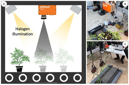
Figure 1.
Schematic diagram of the hyperspectral imaging system with a conveyor belt and two halogen light sources for measuring plants (A), potted potato (B), and potted wheat (C) plants being measured with the hyperspectral camera.
2.2. Preprocessing
The hyperspectral dataset was first corrected using a white reference scan (100% reflectance tile, Tec5 Technology for Spectroscopy, Germany) and a dark reference value (achieved by closing the camera shutter). The data were then subjected to Savitzky–Golay smoothing (polyorder 3, window 33) using the scikit-learn Python package [19]. To remove noisy bands with high, random variation in the measured reflectance, the first 20 and last 30 wavebands were removed from the wheat and potato datasets, resulting in 174 wavebands. The dataset was then normalised between 0 and 1 using the scikit-learn package. The normalisation step needed to be performed after removing noisy bands, since these bands adversely affect normalisation. Soil pixels were deleted based on the 718 nm band of the first derivative reflectance spectrum for the wheat dataset, and the 527 and 718 nm bands of the first derivative spectrum for the potato dataset. These bands were identified iteratively, selecting wavebands that appeared to differ between crops and soil, based on a plot of soil spectra versus plant spectra, and using threshold values for these bands to segment the image. This was possible by visually selecting soil pixels that were clear on the red, green, and blue (RGB) representation hyperspectral image and comparing their spectrum with that of plant pixels. The quality of soil pixel segmentation was assessed by visual inspection of the image and plotting of spectra belonging to the remaining pixels and comparing these to known soil spectra.
2.3. Training Set Construction
For the manually labelled dataset, the Lasso Selector functionality of the matplotlib Python package [20] was used to select the ROI and store the spectral signatures in separate datasets. A region containing clear disease symptoms surrounded by a relatively healthy leaf tissue was selected from the hyperspectral image (Figure 2A). From this region containing both healthy and infected leaves from one plant, five ROIs were selected at an increasing distance from the centre of the rust or P. infestans lesion (Figure 2B). These regions were labelled from stage 5 (most diseased) to stage 1 (least diseased) by hand using the Lasso Selector function in matplotlib. Note that apart from the most severe stages (stages 4 and 5), symptoms were not visible to the naked eye, and an estimation of disease intensity was made based on the distance from the centre of the lesion. The entire core of the clearly visible symptom (here, a durum wheat striped rust lesion with an orange color) was labelled as stage 5. The adjacent regions were progressively labelled as stages 4 to 2 with stage 1 being pixels from a neighbouring leaf that did not show clear rust symptoms.

Figure 2.
Red, green, and blue (RGB) representation of a hyperspectral image after preprocessing and soil and background removal. The red square (A) shows the region of interest (ROI) that was used to manually label a relatively small training dataset for a comparison with the automatic labelling algorithm. This ROI is enlarged in the image on (B).
These five datasets were then combined to form the hyperspectral training library. Note that in Figure 2, the striped rust disease progressed from the tip of the leaf in a striped pattern farther toward the centre of the plant. This indicated that the highest disease stage was at the tip of the wheat leaf, the lower at the centre of that leaf, and the healthy or stage 1 ROI was positioned on an adjacent leaf without rust symptoms. This resulted in the ‘manually labelled’ hyperspectral training library. The sizes of the training sets were comparable among classes so as to not affect the model training. Otherwise, the ‘class_weight’ feature of the logistic regression should be set to ‘balanced’ to adjust training set weights based on the difference in sample size.
For the automatic labelling algorithm, a series of wavebands was selected by plotting a cross section over a region of pixels containing the full development from healthy-looking wheat or potato tissue to clearly diseased pixels (Figure 3). This is based on the fact that the disease spreads from an initial infection site, growing throughout the leaf in a concentric pattern (P. infestans on potato) or a directional pattern (leaf rust on wheat). Therefore, the area surrounding the initial infection site represents gradually less and less diseased plant tissue farther from the initial infection site. This leads to the plot in Figure 3, which represents the change in the hyperspectral signature as disease progresses and shows regions of the spectrum that vary most during disease progression. Based on this cross-section plot, wavebands were identified where the reflectance appeared to vary with the disease progression. For each of the bands selected in this way, the minimum, standard deviation, and mean of the reflectance were calculated over the entire image (for wheat) or over a specific ROI containing the disease symptoms (for potatoes). To avoid outliers, the maximum value over the entire image was set to be equal to the mean plus two times the standard deviation. The difference between the maximum and minimum reflectance values for the band in question were then divided by 5 (or any other desired number of training classes) to obtain a step size. Using this step size, each pixel was assigned a label between 1 and 5, based on whether the reflectance value for that pixel was positioned between the minimum and the minimum + 1 * step size, between the minimum + 1 * step size and the minimum + 2 * step size, between the minimum + 2 * step size and the minimum + 3 * step size, and so on. If the maximum value for this band corresponded with diseased pixels, the pixels with the high reflectance values were automatically labelled ‘5’, whereas healthier pixels with a low reflectance were labelled ‘1’. For wavebands where a low reflectance corresponded with diseased pixels, the pixels with high reflectance values were labelled ‘1’, whereas healthier pixels with a higher reflectance were labelled ‘5’ (Figure 4).
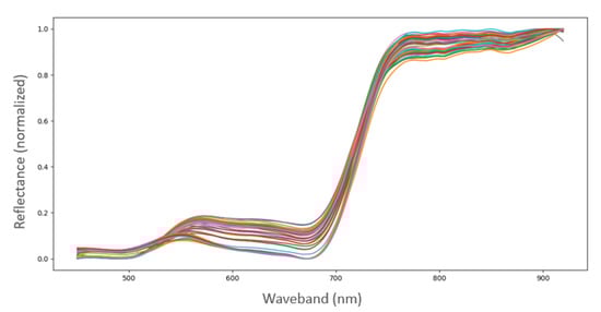
Figure 3.
Plot of the hyperspectral signatures spanning an area of the leaf containing healthy wheat tissue, rust disease, and the transition zone between the two. Spectral signatures are shown after preprocessing (cutting noisy bands, Savitzky–Golay smoothing and normalization). Each curve represents the spectral signature of a pixel in the cross section of the area, with pixels ranging from healthy to fully diseased.

Figure 4.
Example of the automatic labelling algorithm. The colour bar represents the label given by the automatic labelling algorithm.
Note that for the potato dataset, only an ROI (with healthy and diseased potato tissues) was used instead of using the full image because several pixels remained after the removal of the soil that interfered with the labelling process. It is possible that these pixels were the decaying plant tissue of older leaves present on the soil surface after being damaged during the experiment.
This automatic labelling process was repeated for all the bands selected (Figure 4A). Figure 4A shows the selection of bands that appeared interesting for disease detection after labelling with the automatic labelling process, based on a visual inspection of the changes in the hyperspectral signature as the disease progressed. Bands that after labelling appeared to show a similarity to the visual presence of the disease were averaged into one average label image. This was performed by, for each pixel, averaging the label value assigned by the automatic labelling algorithm based on each waveband (Figure 4B). The spectra and averaged band labels belonging to the pixels in Figure 4B were then extracted and organised in the automatically labelled hyperspectral training library. Bands that did not appear to match the visible disease pattern were excluded (760 nm band, Figure 4A). Red edge bands 2 and 3 are ratios of the 667 nm band to the 760 nm band and of the 667 nm band to the 550 nm band, respectively.
2.4. Modelling
After preprocessing and manual or automatic labelling, the resulting training datasets were used to train a logistic regression model using the LogisticRegressionCV function of the scikit-learn Python package [21]. The polyorder was set to 2, and the training window was set to 33. Seven C-values (0.1, 0.5, 1, 1.5, 2, 4, and 10) were provided for the model, which automatically selected the optimal C-value. To first compare the model performance between the automatic and manual labelling. The full spectrum was used for training based on both the manually and automatically labelled training sets.
To explore the potential of selecting a reduced number of wavebands on (a) improving the classification accuracy and (b) reducing data and processing needs, six classification scenarios were compared using the potato dataset (because clearer presence of visual disease symptoms made manual labelling more reliable). Variations in the training included:
- 1
- Training on an ROI spanning one infected leaf or a ‘composite’ image composed of a combination of hyperspectral images of the same plant obtained on different measurement days over the entire experiment duration;
- 2
- Training on the full spectrum or on two selected bands that appeared most promising during the automatic labelling process (760 and 550 nm);
- 3
- Training using the manual or automatic training label assignment.
The manually labelled training library was not altered. A new automatically labelled training library was constructed but based on a composite hyperspectral image. This composite image was created by combining the ROIs from hyperspectral images obtained during 0, 4, 7, 11, and 16 days postinfection. The automatic labelling algorithm was then used to label the entire composite using the 760 and 550 nm bands to create the average labels. This created a new composite automatically labelled training library.
The three training libraries (based on one image, manually labelled; based on one image, automatically labelled; and based on a composite image, automatically labelled) were then each used as an input for the logistic regression model with the same preprocessing steps using both the full spectrum and only two features (760 and 550 nm) instead of the full spectrum. The classification result was then compared based on the classification accuracy (with 70% of the training set used for model training and 30% used for validation), the confusion matrix the metrics (such as false-positive rate) calculated from the confusion matrix, and by visual assessment of symptom classification by comparing visible symptoms with the classification result.
3. Results
3.1. Wheat
For the soft wheat dataset, the automatic labelling algorithm provided three images of bands or band ratios with labels that matched the visual presence of the disease: the 667 nm band, red edge band 2 (a ratio of the 667 nm band to the 760 nm band), and red edge band 3 (a ratio of the 667 nm band to the 550 nm band) (Figure 4A). The reflectance in these three bands appeared to correlate well with the visual symptoms present in the hyperspectral image (Figure 2A).
For each of the trained models, a confusion matrix was calculated to assess the model performance (Figure 5). Note that only one confusion matrix is shown, but the analysis of the models was based on the confusion matrix of each model. The manually trained model showed a greater number of misclassifications compared with the automatically labelled model especially for disease stages 1 and 2. For disease stages 3 and 4, it performed with a slightly higher accuracy.
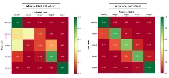
Figure 5.
Comparison of the confusion matrices showing the result of the manually labelled and automatically labelled disease detection models for rust disease on soft wheat. The values shown are normalised, showing the percentage of the true label that was classified as each of the five classes. Note that classes were renamed to healthy, stage 1, stage 2, stage 3, and stage 4 instead of numbers 1 to 5 to indicate that label 1 corresponded with the healthiest pixels, whereas label 5 corresponded with the most advanced disease stage.
The model trained on the labels of the averaged label image (Figure 4B) reached a training accuracy of 97.69%. The model trained on the manually labelled dataset (with the same parameters) achieved a lower accuracy of 96.33%. When comparing the classification results of both models with a new image (not used for model training), the manual model performed 1.36% less accurately compared with the automatic model and seemed to less clearly classify the visible rust symptoms (Figure 6).
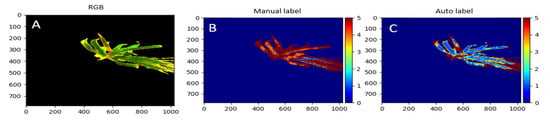
Figure 6.
Comparison for soft wheat of the performances of the manually labelled model (B) with the automatically labelled model (C) with the red, green, and blue (RGB) representation of the hyperspectral image (A). Both the manually and automatically labelled datasets were fed into a logistic regression model, obtaining classification accuracies of 96.33% and 97.69% for the manual and automatic models, respectively. The color bar represents the label given by the automatic labelling algorithm.
For durum wheat, the same three bands were selected during automatic labelling. The training accuracy achieved with this automatically labelled model was 96.66%. The manually labelled model had a lower accuracy of 86.42%. The manual labelling model also showed clear signs of misclassification where shaded areas were classified as disease (Figure 7).

Figure 7.
Comparison for durum wheat of the performances of the manually labelled model (B) with the automatically labelled model (C) with the red, green, and blue (RGB) representation of the hyperspectral image (A). Both the manually and automatically labelled datasets were fed into a logistic regression model, obtaining classification accuracies of 86.42% and 96.66% for the manual and automatic models, respectively. The color bar represents the label given by the automatic labelling algorithm.
3.2. Potato
For the potato dataset, the automatic labelling algorithm indicated two bands that showed labels matching the visible symptoms, namely, red edge band 2 and red edge band 3. Figure 8 shows the classification results of the manually labelled model and the automatically labelled model for potato. The manually labelled model achieved a classification accuracy of 79.45%, whereas the automatically labelled model achieved an accuracy of 98.80%. Not only was the classification accuracy of the manually labelled model lower than that of the automatically labelled model, but it also showed clear patterns where shading and angle effects affected the classification. These regions were even shown as a stage 3 disease in a few places.
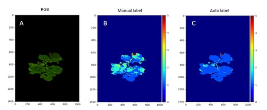
Figure 8.
Comparison of the performances of the manually labelled model (B) with the automatically labelled model (C) with the red, green, and blue (RGB) representation of the hyperspectral image (A). Both the manually and automatically labelled datasets were fed into a logistic regression model with classification accuracies of 79.45% and 98.80% for the manual and automatic models, respectively. The color bar represents the label given by the automatic labelling algorithm.
3.3. Model Performance Comparison
Figure 9 shows a comparison of the models trained using six different training sets. The model accuracies are shown in the figure caption and in Table 1. Note that the automatically trained models performed more accurately by around 20% compared with the manually trained models. None of the automatically trained models performed under 98% accuracy, and the composite image-trained automatically labelled model using the full spectrum performed best with 99.83% accuracy.
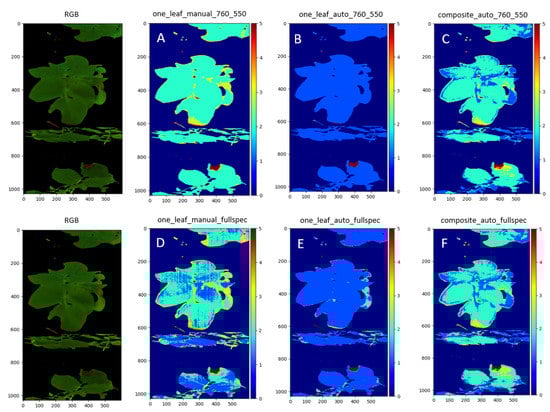
Figure 9.
Comparison of the performance of the manually labelled model with the automatically labelled model with the red, green, and blue (RGB) representation of the hyperspectral image. (A) to (F) represent the classification results of the models trained on six different training sets with variations between them in the number of features used, with two features (A–C) compared with the full spectrum (D–F), the training set being an automatically labelled training set based on a region of interest of one measurement day (B,E) or on a region of interest of a composite image spanning the duration of the experiment (C,F) or based on a manually labelled training set (A,D). Model accuracies: 72.10% (A), 98.06% (B), 99.48% (C), 79.45% (D), 99.80% (E), and 99.83% (F). The color bar represents the label given by the automatic labelling algorithm.

Table 1.
Model accuracies for each of the six tested models calculated on a 70/30 split for model training and validation, respectively. The full-spectrum models incorporated all 174 wavebands retained after cutting the noisy part of the spectrum (keeping the wavebands between 450 and 920 nm). The two-feature models incorporated only two wavebands: 760 and 550 nm. These models were both trained on each of three datasets: a dataset from a single ROI spanning one leaf that showed healthy and diseased tissues (one leaf dataset) that was either manually labelled or automatically labelled using the automatic labelling algorithm and a dataset from a composite image that combined several ROIs over the entire experiment duration.
4. Discussion
During the asymptomatic stage of disease development (incubation period), physiological processes (e.g., stomatal closure) can be affected at the cellular level. The bands used in this study are located in the visible/near-infrared wavelength range. The reflectance in this spectral zone is sensitive to the changes in foliar pigments (photosynthetically active plant components) according to Devadas et al. [22]. The destruction of these pigments directly influences the absorption and conversion of light energy [23]. Zubler and Jhon (2020) [24] noticed that cellular changes in the convexity of the epidermal cell, surface texture, thickness of the leaf cuticle, and cell wall elasticity can influence reflectance values. These changes affect stomatal processes, reducing stomatal conductance and CO2 concentration [25].
The finding that red edge band 2 and red edge band 3 were used in the labelling of P. infestans in potatoes and both rust diseases in wheat could suggest that these bands are possibly universally applicable for disease detection. This is logical as these ratio bands incorporate information from the 550, 667, and 760 nm bands. This is supported by the literature where reflectance measurements in 20 nm bands surrounding the 543, 630, 680, 725, 750, and 861 nm bands have been used to create models with 99% classification accuracy [26,27]. This is further supported by the fact that the 550, 667, and 760 nm bands are commonly used in vegetation indices [27,28]. For the labelling of the composite image, these bands performed well but worse than the pure 760 and 550 nm band combination without ratios.
Looking at the results in Figure 9, it is clear that the models trained on the automatically labelled composite image did not necessarily achieve higher classification accuracies than the models trained on the automatically labelled regions of interest spanning a single leaf with disease symptoms with accuracies of 99.80% for the autolabelled one leaf model and 99.83% for the autolabelled composite model (using the full spectrum). The results shown in Figure 9C,F also suggest that it is possible to reduce data storage and processing needs by selecting just two features (750 and 550 nm) with the classification accuracy dropping only slightly from 99.83% to 99.48% by reducing the number of features from 174 to 2.
Scientists have progressed in using semisupervised learning methods. One problem with these methods is that they are relatively complex and require expert knowledge, which is not always available to phytopathologists studying crop diseases. For example, Zhang et al. [29] developed a methodology based on multiple Inception-Resnet layers for detecting yellow rust in winter wheat, achieving an accuracy of 85%. More recent is the study carried out by Pan et al. [30], where a semantic segmentation model called pyramid scene parsing network (PSPNet) reached high accuracy (greater than 98%), identifying yellow rust as well. Both methods require costly computer resources, and the resolution at field level is also a factor that must be considered. The method proposed in the current work is less complex by comparison and is more intuitive. Semisupervised machine learning methods still require experts to label a small subset of the training data for the unsupervised learning process. In the case of active learning, expert input is needed throughout the process, which is costly and hard to automate. The method in the current work could potentially be used as an additional step to automatically create a relatively large starting training set, after which semisupervised machine learning methods could be used without the need for user input.
Looking at the comparison of classifications for all three diseases, it became clear that the automatically labelled classification always outperformed the manually labelled classification in terms of overall accuracy (Figure 6, Figure 7 and Figure 8). More importantly, a comparison of the confusion matrices of these classifications, such as the example in Figure 5, showed that there were fewer misclassifications in the moderate disease stages (labelled 2–4 in Figure 6, Figure 7 and Figure 8) for the models trained on automatically labelled data. This is important when the aim is to establish whether the pathogen is still actively growing in the crop because this signifies the transition stages of the disease. This can be an important factor in the decision-making process and can affect the decision to apply fungicides in the field.
The automation potential of the solution in the current work was further emphasised by the finding that red edge band 2 and red edge band 3 ratios seemed to be universally applicable. In theory, if a region of a field is known to have both diseased and healthy plants, it is possible to scan this area with a hyperspectral camera and use these data as the input for the automatic labelling algorithm. As this algorithm works based on the minimum and maximum (after the outlier removal) of these two bands, there is no need for human intervention to label the pixels from this scanned area and train the machine learning classifier. This could, in theory, automate the manner in which autonomous rovers can detect diseases in the field, regardless of the crop or pathogen. In such cases, the training set could be automatically constructed, used to train a machine learning classifier, and applied to map the spread of disease in the field without human intervention. However, many practical issues regarding the presence of combined sources of crop stress (both biotic and abiotic) would need to be overcome. Future experiments should therefore focus on testing the effectiveness of the method presented in this work in a variety of conditions.
5. Conclusions
The automatic labelling strategy proposed in this work presents a relatively simple and intuitive method of automating the construction of hyperspectral training sets. The effectiveness of this method was tested on hyperspectral images of potato and wheat plants infected with P. infestans and P. triticina, respectively. These datasets were subjected to manual labelling and automatic labelling and used as an input for a logistic regression machine learning model using Python. The modelling accuracies of the automatically labelled datasets were higher than those of the manually labelled ones for both potatoes and wheat, at 98.80% for P. infestans in potato, 97.69% for rust in soft wheat, and 96.66% for rust in durum wheat. When examining the final classified image, the automatically labelled models performed with a higher accuracy and fewer misclassifications due to shading and angle effects. This method could provide a supplementary step for semisupervised machine learning, eliminating the need for expensive expert labelling. The exclusion of human intervention opens further possibilities for automatic disease detection using robots in field conditions where a model could be trained directly on the hyperspectral measurements of the field. However, many practical constraints, such as the presence of mixed biotic and abiotic stresses, need to be examined in future studies.
Author Contributions
All authors contributed to the article and approved the submitted version. S.A. wrote the first draft of the paper, took the field measurements, prepared the hardware and software, and analysed the data; O.E.A.-A. took the field measurements and logistic procedures, prepared the hardware and software, and provided suggestions on the manuscript; J.N.R.-V. took the field measurements and conceived the wheat experiments; M.P.-R. conceived both experiments, supervised, and acquired funding; J.P. and A.M.M. provided suggestions on the structure of the manuscript, participated in the discussions of the results, and acquired funding. All authors have read and agreed to the published version of the manuscript.
Funding
The authors disclose receipt of the following financial support for the research, authorship, and/or publication of this article: this work was supported by the Research Foundation-Flanders (FWO) for Odysseus I SiTeMan Project (Nr. G0F9216N) and the Junta de Andalucía (PROJECT: US-1263678).
Acknowledgments
The authors want to thank the Predoctoral Research Fellowship for the development of the University of Seville R&D&I program (IV.3 2017) granted to O.E.A.-A.
Conflicts of Interest
The authors declare that the research was conducted in the absence of any commercial or financial relationships that could be construed as potential conflicts of interest.
References
- Chen, X. Pathogens which threaten food security: Puccinia striiformis, the wheat stripe rust pathogen. Food Secur. 2020, 12, 239–251. [Google Scholar] [CrossRef]
- Mahlein, A.K.; Oerke, E.C.; Steiner, U.; Dehne, H.W. Recent advances in sensing plant diseases for precision crop protection. Eur. J. Plant Pathol. 2012, 133, 197–209. [Google Scholar] [CrossRef]
- Nagaraju, M.; Chawla, P. Systematic review of deep learning techniques in plant disease detection. Int. J. Syst. Assur. Eng. Manag. 2020, 11, 547–560. [Google Scholar] [CrossRef]
- Bravo, C.; Moshou, D.; Oberti, R.; West, J.; McCartney, A.; Bodria, L.; Ramon, H. Foliar disease detection in the field using optical sensor fusion. Manuscript FP 04 008. Agric. Eng. Int. CIGR J. 2004, VI. [Google Scholar]
- Yuan, L.; Huang, Y.; Loraamm, R.W.; Nie, C.; Wang, J.; Zhang, J. Spectral analysis of winter wheat leaves for detection and differentiation of diseases and insects. F. Crop. Res. 2014, 156, 199–207. [Google Scholar] [CrossRef] [Green Version]
- Krishna, G.; Sahoo, R.N.; Pargal, S.; Gupta, V.K.; Sinha, P.; Bhagat, S.; Saharan, M.S.; Singh, R.; Chattopadhyay, C. Assessing wheat yellow rust disease through hyperspectral remote sensing. In Proceedings of the International Archives of the Photogrammetry, Remote Sensing and Spatial Information Sciences—ISPRS Archives, Hyderabad, India, 9 – 12 December 2014. [Google Scholar]
- Bravo, C.; Moshou, D.; West, J.; McCartney, A.; Ramon, H. Early disease detection in wheat fields using spectral reflectance. Biosyst. Eng. 2003, 84, 137–145. [Google Scholar] [CrossRef]
- Whetton, R.L.; Waine, T.W.; Mouazen, A.M. Hyperspectral measurements of yellow rust and fusarium head blight in cereal crops: Part 2: On-line field measurement. Biosyst. Eng. 2018, 167, 144–158. [Google Scholar] [CrossRef] [Green Version]
- Gold, K.M.; Townsend, P.A.; Chlus, A.; Herrmann, I.; Couture, J.J.; Larson, E.R.; Gevens, A.J. Hyperspectral measurements enable pre-symptomatic detection and differentiation of contrasting physiological effects of late blight and early blight in potato. Remote Sens. 2020, 12, 286. [Google Scholar] [CrossRef] [Green Version]
- Franceschini, M.H.D.; Bartholomeus, H.; van Apeldoorn, D.F.; Suomalainen, J.; Kooistra, L. Feasibility of unmanned aerial vehicle optical imagery for early detection and severity assessment of late blight in Potato. Remote Sens. 2019, 11, 224. [Google Scholar] [CrossRef] [Green Version]
- Sugiura, R.; Tsuda, S.; Tamiya, S.; Itoh, A.; Nishiwaki, K.; Murakami, N.; Shibuya, Y.; Hirafujia, M.; Nuske, S. Field phenotyping system for the assessment of potato late blight resistance using RGB imagery from an unmanned aerial vehicle. Biosyst. Eng. 2016, 148, 1–10. [Google Scholar] [CrossRef]
- Ray, S.S.; Jain, N.; Arora, R.K.; Chavan, S.; Panigrahy, S. Utility of Hyperspectral Data for Potato Late Blight Disease Detection. J. Indian Soc. Remote Sens. 2011, 39, 161–169. [Google Scholar] [CrossRef]
- Paulus, S.; Mahlein, A.K. Technical workflows for hyperspectral plant image assessment and processing on the greenhouse and laboratory scale. Gigascience 2020, 9, giaa090. [Google Scholar] [CrossRef]
- Appeltans, S.; Pieters, J.G.; Mouazen, A.M. Detection of leek rust disease under field conditions using hyperspectral proximal sensing and machine learning. Remote Sens. 2021, 13, 1341. [Google Scholar] [CrossRef]
- Rajadell, O.; García-Sevilla, P.; Dinh, V.C.; Duin, R.P.W. Improving hyperspectral pixel classification with unsupervised training data selection. IEEE Geosci. Remote Sens. Lett. 2014, 11, 656–660. [Google Scholar] [CrossRef] [Green Version]
- Joalland, S.; Screpanti, C.; Liebisch, F.; Varella, H.V.; Gaume, A.; Walter, A. Comparison of visible im-aging, thermography and spectrometry methods to evaluate the effect of Heterodera schachtii inoculation on sugar beets. Plant Methods 2017, 13, 73. [Google Scholar] [CrossRef]
- Wu, Y.; Mu, G.; Qin, C.; Miao, Q.; Ma, W.; Zhang, X. Semi-supervised hyperspectral image classification via spatial-regulated self-training. Remote Sens. 2020, 12, 159. [Google Scholar] [CrossRef] [Green Version]
- Ma, X.; Geng, J.; Wang, H. Hyperspectral image classification via contextual deep learning. EURASIP J. Image Video Process. 2015, 2015, 20. [Google Scholar] [CrossRef] [Green Version]
- Dópido, I.; Li, J.; Plaza, A.; Bioucas-Dias, J.M. A new semi-supervised approach for hyperspectral image classification with different active learning strategies. In Proceedings of the 4th Workshop on Hyperspectral Image and Signal Processing, Evolution in Remote Sensing (WHISPERS) (pp. 1–4). IEEE., Shanghai, China, 4–7 June 2012. [Google Scholar]
- Hunter, J.D. Matplotlib: A 2D graphics environment. Comput. Sci. Eng. 2007, 9, 90–95. [Google Scholar] [CrossRef]
- Pedregosa, F.; Varoquaux, G.; Gramfort, A.; Michel, V.; Thirion, B.; Grisel, O.; Blondel, M.; Prettenhofer, P.; Weiss, R.; Dubourg, V.; et al. Scikit-learn: Machine Learning in Python. JMLR 2011, 12, 2825–2830. [Google Scholar]
- Devadas, R.; Lamb, D.W.; Simpfendorfer, S.; Backhouse, D. Evaluating ten spectral vegetation indices for identifying rust infection in individual wheat leaves. Precis. Agric. 2009, 10, 459–470. [Google Scholar] [CrossRef]
- Marín-Ortiz, J.C.; Gutierrez-Toro, N.; Botero-Fernández, V.; Hoyos-Carvajal, L.M. Linking physiological parameters with visible/near-infrared leaf reflectance in the incubation period of vascular wilt disease. Saudi J. Biol. Sci. 2020, 27, 88–99. [Google Scholar] [CrossRef]
- Zubler, A.V.; Yoon, J.Y. Proximal Methods for Plant Stress Detection Using Optical Sensors and Machine Learning. Biosensors 2020, 10, 193. [Google Scholar] [CrossRef]
- Carretero, R.; Bancal, M.O.; Miralles, D.J. Effect of leaf rust (Puccinia triticina) on photosynthesis and related processes of leaves in wheat crops grown at two contrasting sites and with different nitrogen levels. Eur. J. Agron. 2011, 35, 237–246. [Google Scholar] [CrossRef]
- Moshou, D.; Bravo, C.; West, J.; Wahlen, S.; McCartney, A.; Ramon, H. Automatic detection of ‘yellow rust’ in wheat using reflectance measurements and neural networks. Comput. Electron. Agric. 2004, 44, 173–188. [Google Scholar] [CrossRef]
- Moshou, D.; Bravo, C.; Oberti, R.; West, J.; Bodria, L.; McCartney, A.; Ramon, H. Plant disease detection based on data fusion of hyper-spectral and multi-spectral fluorescence imaging using Kohonen maps. Real-Time Imaging 2005, 11, 75–83. [Google Scholar] [CrossRef]
- Franceschini, M.H.D.; Bartholomeus, H.; van Apeldoorn, D.; Suomalainen, J.; Kooistra, L. Intercomparison of unmanned aerial vehicle and ground-based narrow band spectrometers applied to crop trait monitoring in organic potato production. Sensors 2017, 17, 1428. [Google Scholar] [CrossRef]
- Zhang, X.; Han, L.; Dong, Y.; Shi, Y.; Huang, W.; Han, L.; González-Moreno, P.; Ma, H.; Ye, H.; Sobeih, T. A deep learning-based approach for automated yellow rust disease detection from high-resolution hyperspectral UAV images. Remote. Sens. 2019, 11, 1554. [Google Scholar] [CrossRef] [Green Version]
- Pan, Q.; Gao, M.; Wu, P.; Yan, J.; Li, S. A Deep-Learning-Based Approach for Wheat Yellow Rust Disease Recognition from Unmanned Aerial Vehicle Images. Sensors 2021, 21, 6540. [Google Scholar] [CrossRef]
Publisher’s Note: MDPI stays neutral with regard to jurisdictional claims in published maps and institutional affiliations. |
© 2021 by the authors. Licensee MDPI, Basel, Switzerland. This article is an open access article distributed under the terms and conditions of the Creative Commons Attribution (CC BY) license (https://creativecommons.org/licenses/by/4.0/).