Machine Learning Algorithms for Modeling and Mapping of Groundwater Pollution Risk: A Study to Reach Water Security and Sustainable Development (Sdg) Goals in a Mediterranean Aquifer System

Abstract

Groundwater pollution poses a severe threat and issue to the environment and humanity overall. That is why mitigative strategies are urgently needed. Today, studies mapping groundwater risk pollution assessment are being developed. In this study, five new hybrid/ensemble machine learning (ML) models are developed, named DRASTIC-Random Forest (RF), DRASTIC-Support Vector Machine (SVM), DRASTIC-Multilayer Perceptron (MLP), DRASTIC-RF-SVM, and DRASTIC-RF-MLP, for groundwater pollution assessment in the Saiss basin, in Morocco. The performances of these models are evaluated using the Receiver Operating Characteristic curve (ROC curve), precision, and accuracy. Based on the results of the ROC curve method, it is indicated that the use of hybrid/ensemble machine learning (ML) models improves the performance of the individual machine learning (ML) algorithms. In effect, the AUC value of the original DRASTIC is 0.51. Furthermore, both hybrid/ensemble models, DRASTIC-RF-MLP (AUC = 0.953) and DRASTIC-RF-SVM, (AUC = 0.901) achieve the best accuracy among the other models, followed by DRASTIC-RF (AUC = 0.852), DRASTIC-SVM (AUC = 0.802), and DRASTIC-MLP (AUC = 0.763). The results delineate areas vulnerable to pollution, which require urgent actions and strategies to improve the environmental and social qualities for the local population.

1. Introduction

Groundwater resources represent a precious source for the life of both humans and animals [1,2]. According to UNICEF [3], it is estimated that about 2.2 billion people globally still have no access to drinking water supply [4]. Groundwater pollution is a worldwide challenge, specifically in arid and semi-arid regions [5,6].

Groundwater pollution is associated with the uncontrolled and irrational use of agrochemicals for agricultural activities [7,8]. Therefore, the applicability of pesticides leads to dangerous effects on both human life and environmental ecosystems [9]. Thus, the use of pesticides for agricultural practices presents a double-edged sword and farmers should be sensitize about following an integrated approach of crop insurance and farmers’ selection of pesticide input [10]. This may be complicated by drought related to climate change impacts, which affect crop yields and decrease groundwater resources [10].

The uncontrolled use of nitrogen fertilizers catalyzes the nitrate leaching, leading to groundwater pollution [11]. The nitrates (NO₃−N) are the most popular indicator for assessing groundwater pollution due to their severe effect on the aquifer; furthermore, they can lead to many effects including methaemoglobinaemia. Ranking the risk of nitrate concentration pollution on a groundwater aquifer is done by the World Health Organization (WHO), i.e., an aquifer receiving a concentration of nitrate exceeding 50 mg/L, is considered polluted [12]. This situation forces researchers to develop a strategy to select areas with the highest risk to vulnerability. Thus, the establishment of spatial vulnerability tools constitutes a crucial opportunity to urgently and easily delineate areas that are highly vulnerable to groundwater pollution and, in doing so, to highlight a need for adequate strategies and decision-making actions to sustainably manage the groundwater resources.

A major portion of modeling studies is complex due to the processing of different data and their size. In this sense, with the many opportunities of the geographic information system (GIS) tools and spatial operations, GIS tools have shown its applicability as a useful space for preprocessing different kinds of spatiotemporal datasets [13,14]. These opportunities greatly assist researchers in achieving their purposes in environmental studies.

Numerous studies have been conducted to assess groundwater vulnerability to pollution based on different methods [15]. Among these, the DRASTIC approach developed by Aller et al. [16], based on seven parameters, including depth to water (D), recharge (R), aquifer media (A), soil media (S), topography (T), impact of the vadose zone (I), and hydraulic conductivity (C), has yielded promising outcomes in many research cases [17,18]. However, the original version of the DRASTIC method has its limitations [19]. As pointed out by Nadiri et al. [20], each aquifer, unconfined or confined, presents its own characteristics (i.e., the aquifer type in terms of geological composition and confined/unconfined nature and the water table depth). Thus, we argue that the applicability of the DRASTIC method in an area presenting both unconfined or confined aquifers becomes difficult regarding the assignments of vulnerability risk and it cannot be generalized.

The fact that each user adopts and adjusts the methodology based on the conditions of the background of the area studied may be another drawback of the applicability of the DRASTIC method. There is no conventional guideline to follow to decide whether the vulnerability index is “right” or “wrong” and the level of the exactitude of the vulnerability index remains unknown. Because of these uncertainties, many researchers have modified the original DRASTIC method to increase its accuracy using several techniques. These include frequency ratio [21], Analytical Hierarchy Process (AHP) [22], Fuzzy-AHP model [1], Single-Parameter Sensitivity Analysis [23], Mamdani Fuzzy Logic (MFL) model [24] and Supervised Committee with Fuzzy Logic model [24], projection pursuit dynamic clustering, and also anthropogenic influence, such as land cover/land use impacts [25].

More recently, hybrid ensemble machine learning (ML) models (i.e., a combination of single methods and statistical techniques) have been developed with promising results in different environmental hazard fields [26,27], such as flood [28,29], landslide [30,31], forest fire susceptibility [32], and groundwater level prediction [33].

To date, there has been no prior study on the use of hybrid machine learning (ML) algorithms (i.e., combination of machine algorithm models and statistical tests) as an opportunity for groundwater pollution studies. In the Saiss basin, where this research was conducted, the local population is largely dependant on agriculture to serve as a source of their livelihood. However, the unsustainable use of pesticides is increasingly affecting the quality and the quantity of water resources in this aquifer.

In this ecosystem, previous efforts have been made by other authors. For instance, Sadkaoui et al. [34] used the DRASTIC, GOD, and PRK methods to assess groundwater vulnerability. They reported the sensitivity of water resources due to the pollution coming from the ground surface. Moreover, a recent article developed by Lahjouj et al. [35] used random forest (RF) to map groundwater vulnerability with encouraging outcomes. With respect to the above cited articles, the work presented here takes a step further in the field of hybridization of machine learning (ML) models and statistical tests. In this case, we proposed five new ensemble models, DRASTIC-RF (random forest), DRASTIC-SVM (support vector machine), DRASTIC-MLP (multilayer perceptron), DRASTIC-RF-SVM, and DRASTIC-RF-MLP for groundwater vulnerability pollution risk assessment in the Saiss basin.

2. Materials and Methods

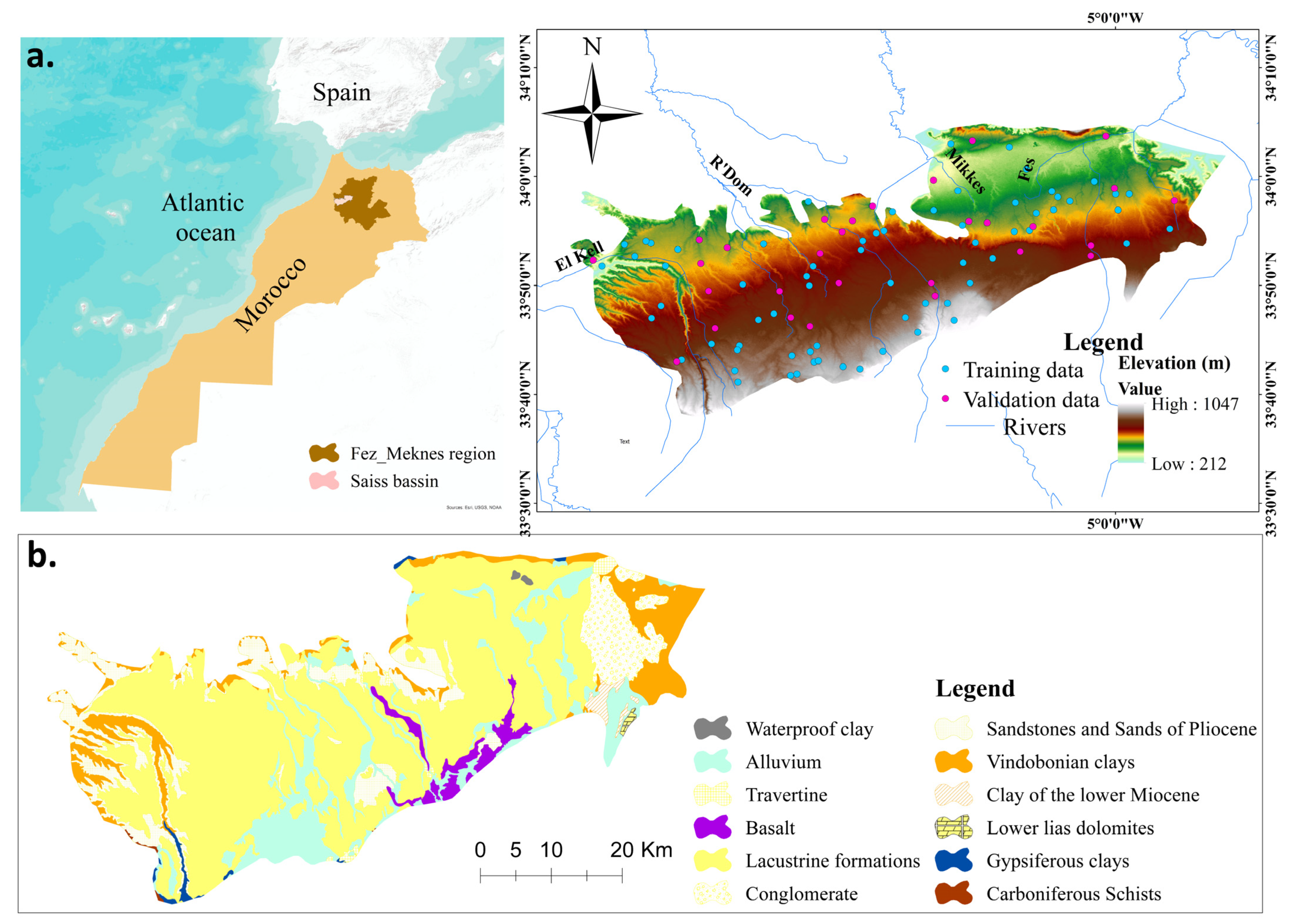
2.1. Study Area

This research was conducted in the Saiss basin, located in the Fez-Meknes region, Morocco (Figure 1), between latitudes 33°38′ N and 34°4′ N and longitudes 5°49′ W and 4°53′ W. The basin occupies an area of about 2100 km². The elevation ranges from 212 to 1047 m. According to Koppen Climate Classification, the study area is characterized by Mediterranean climate and it has an average annual temperature of 17.2 °C, recorded in Meknes station. The average annual precipitation is about 589.3 mm. According to the census report of 2014, the population is about 2.3 million inhabitants.

From the geological point of view, the Saiss comprises several formations extending from the Palaeozoic to the Quaternary, the majority of which are Pliocene Lake limestones and fawn sands [37]. The hydrographic network of the basin consists of four main wadis, which are Oued El Kell, Oued Mikkes, Oued R’Dom, and Oued Fes. According to Essahlaoui et al. [37], the Saiss aquifer system presents a complex structure of two aquifers: the Plioquaternary phreatic aquifer composed of Pliovillafranchian sandstone, conglomerated sand and lacustrine limestone, and the liassic aquifer composed of dolomitic limestone. In this aquifer, as agriculture is still going to be one of the main sources of the local population, to meet the livelihood’s resource requirements, more comprehensive studies should be carried out to promote the sustainable use of natural resources for the proper management and planning of them.

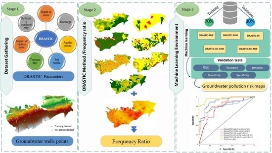
2.2. Data Used and Methodology

The methodology followed in this work is composed of the following stages. The first step of this study was the use of DRASTIC method to map and assess groundwater vulnerability to pollution. Next, the bivariate statistic frequency ratio was applied to modify the result of DRASTIC method. Then, five new hybrid/ensemble machine learning models, namely DRASTIC-RF, DRASTIC-SVM, DRASTIC-MLP, DRASTIC-RF-SVM, and DRASTIC-RF-MLP, were proposed and developed in Python and the Jupyter Notebook Environment. Finally, groundwater vulnerability pollution risk maps were carried out.

2.3. Assessment of Groundwater Vulnerability to Pollution Using DRASTIC Method

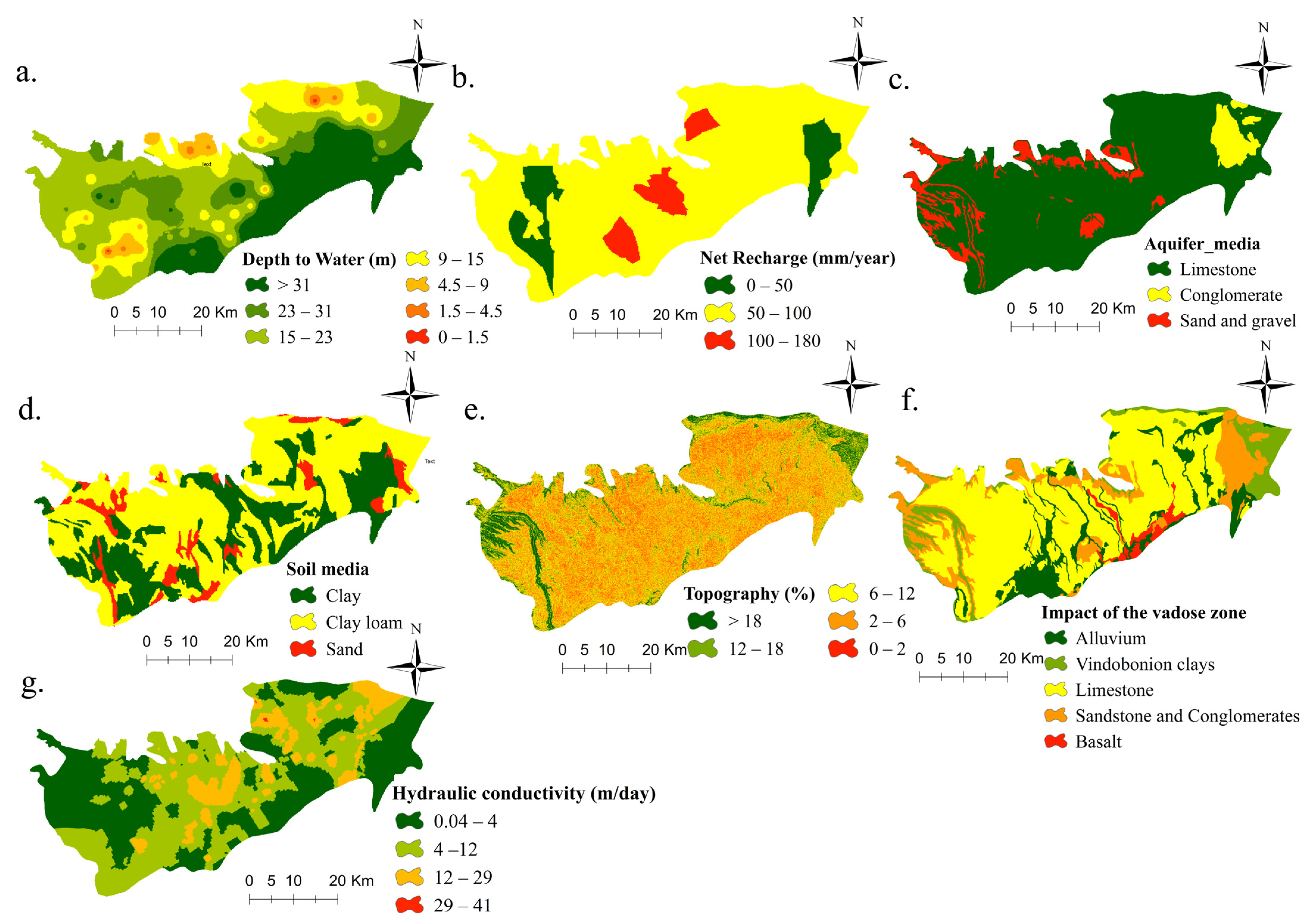
2.3.1. DRASTIC Method and Parameters Description

DRASTIC method is a widely applied approach to assess groundwater vulnerability [21]. It is based on seven factors (Figure 2), including depth to groundwater (D), net recharge (R), aquifer media (A), soil media (S), topography (T), impact of the vadose zone (I), and hydraulic conductivity (C). Following the classification established by Aller et al. [16], different rates (r) and weights (w) are assigned to each class of each DRASTIC parameter. The DRASTIC method was calculated using Equation (1):

$$\mathrm{DRASTIC}={\mathrm{D}}_{\mathrm{r}}{\mathrm{D}}_{\mathrm{w}}+{\mathrm{R}}_{\mathrm{r}}\mathrm{R}+{\mathrm{A}}_{\mathrm{r}}{\mathrm{A}}_{\mathrm{w}}+{\mathrm{S}}_{\mathrm{r}}\mathrm{S}+{\mathrm{T}}_{\mathrm{r}}{\mathrm{T}}_{\mathrm{w}}+{\mathrm{I}}_{\mathrm{r}}{\mathrm{I}}_{\mathrm{w}}+{\mathrm{C}}_{\mathrm{r}}\mathrm{C}$$

(1)

where r is the parameter rate and w is the parameter weight.

• Depth to groundwater (D)

According to Khosravi [21], the (D) parameter presents the distance measured from ground surface to water table. It is considered a limiting factor for groundwater vulnerability, because it conditions the transfer process of pollutant and its possibility of degradation [17]. The greater the depth of water level, the lower the risk of groundwater vulnerability to pollution [16]. In our case, the depth to water map (Figure 2a) was derived from the Digital Elevation Model (DEM) with a pixel size of 30 m and the piezometric map. Based on the DRASTIC framework range value, the map generated was classified into 7 classes, including 0–1.5 m, 1.5–4.5 m, 4.5–9 m, 9–15 m, 15–33 m, 23–31 m, and >31 m.

• Recharge (R)

The recharge is a hydrological process and corresponds to the amount of water that infiltrates through the surface of the ground and contributes to the recharge of the aquifer [16]. The increase in net recharge leads to an increase in the risk of contamination of groundwater. This parameter is related to the topography and the nature of the geological formations. Net Recharge of the Plio-Quaternary aquifer of the Saiss basin is mainly contributed by precipitation and infiltration of irrigation water, as well as by the drainage of the Liasic aquifer of the Middle Atlassic Causse in the southern part of the Saiss basin [34]. The equation for calculating the net recharge was given by Scanlon et al. [38] as:

$$\mathrm{R}=\mathrm{Sy}\frac{\mathrm{\Delta }\mathrm{h}}{\mathrm{\Delta }\mathrm{t}}$$

(2)

where ${\mathrm{S}}_{\mathrm{y}}$ represents the specific yield, $\mathrm{\Delta }\mathrm{h}$ represents the differences of the water-table height for the highest and lowest tables, and $\mathrm{\Delta }\mathrm{t}$ represents the interval time for those tables.

The net recharge map obtained was divided into 3 classes, including 0–50, 50–100, and 100–180 mm (Figure 2b).

• Aquifer media (A)

The aquifer environment or the saturated zone (see in Figure 2c) influences the vulnerability to pollution because its properties make it possible to control the concentration of pollutants by diluting them. The Saiss aquifer consists of lacustrine formations, conglomerates, sandstones, and sands. These formations are extracted from the Hydrogeological map of the Meknes-Fes basin obtained from Morocco’s National Irrigation Office, Directorate General of Studies (1/100,000).

• Soil (S)

Soil texture affects the amount of infiltration from ground surface. In this study, this parameter was constructed using the pedological map of central Morocco obtained from the national institute of agronomic research, physical environment department (1/500,000). The soils of this study area were divided into 3 classes (see Figure 2d): clay, clay loam, and sand. Areas with sand are characterized by high permeability, whereas clay areas are characterized by lower permeability.

• Topography (T)

Topography parameter plays an important role in the infiltration at the ground surface. A lower slope results in more infiltration and therefore a higher potential for contamination. The slope of the Saiss basin (see in Figure 2e) was extracted from Digital Elevation Model with pixel size 30 m and it ranges from 0% to 112%.

• Impact of Vadose zone (I)

The vadose zone (see in Figure 2f) represents the zone located between the surface of the earth and the upper part of the aquifer; using its property of permeability, it can determine the potential of groundwater contamination. In this research, this layer is constituted by Quaternary formation, such as: impermeable clays, alluviums, travertines, and basalts.

Geological data are obtained from the Hydrogeological map of the Meknes-Fes basin obtained from Morocco’s National Irrigation Office, Directorate General of Studies (1/100,000).

• Hydraulic conductivity (I)

Hydraulic conductivity or permeability presents the capacity of an aquifer to transmit water in a porous medium. The higher C is, the faster the pollutant will be transported. In our case, the hydraulic conductivity is given by Equation (3) [39]:

$$\mathrm{K}=\frac{\mathrm{t}}{\mathrm{b}},$$

(3)

where K represents the hydraulic conductivity (m/s), t represents the transmissivity (m²/s), and b is the aquifer thickness (m). The hydraulic conductivity values in the Sais basin ranged from 0 to 30 m/day (Figure 2g). These values were classified into 4 classes: 0.04–4, 4–12, 12–29, and 29–41 (m/s).

2.3.2. Frequency Ratio

Due to its ease of applicability and understanding [40], the bivariate statistic test frequency ratio is widely used in several hazard monitoring studies [41]. In this study, it was used to understand the spatial correlation between each parameter of DRASTIC method and the nitrate points.

$$\mathrm{FR}=\frac{\frac{{\mathrm{S}}_{\mathrm{f}}}{\mathrm{\Delta }{\mathrm{S}}_{\mathrm{f}}}}{\frac{{\mathrm{N}}_{\mathrm{f}}}{\mathsf{\epsilon }\mathrm{N}}},$$

(4)

where ${\mathrm{S}}_{\mathrm{f}}$ represent the area of each class for each DRASTIC parameter; $\mathrm{\Delta }{\mathrm{S}}_{\mathrm{f}}$ represent the total area of each parameter; ${\mathrm{N}}_{\mathrm{f}}$ represent concentration of nitrate occurrence in the class of each parameter; $\mathrm{\epsilon }$N represent the number of total nitrates in the study area. The correlation between the independent variable, i.e., DRASTIC parameter and the target, i.e., nitrate sample is highest if the FR is >1, whereas the correlation is low if the FR is <1.

The FR was calculated for the rate of each class of each DRASTIC parameter and reclassified using natural breaks method in spatial analyst tools in ArcGIS 10.5 (ESRI; Redlands, CA, USA). Thus, we proposed an improved result for groundwater vulnerability based on statistical approach (

Table 1. Frequency ratio of DRASTIC parameters.

DRASTIC Factors	Class	Weight	No of Nitrate Point	No. of Pixels in Class	FR
D: Depth to water table (m)	>31	5	11	684,246	0.20
	23–31		3	509,395	0.07
	15–23		15	1,051,753	0.18
	9–15		11	468,340	0.29
	4.5–9		3	139,093	0.27
	1.5–4.5		0	13,853	0
	0–1.5		0	994	0
R: Net Recharge (mm)	0–50	4	4	303,233	0.09
	50–100		38	2,371,682	0.88
	100–180		1	191,799	0.02
A: Aquifer media	Limestone	3	34	2,497,029	0.79
	Conglomerate		1	67,596	0. 02
	Sand and gravel		8	302,011	0.19
S: Soil	Clay	2	15	915,874	0.35
	Clay loam		26	1,712,526	0.60
	Sand		2	239,594	0.05
T: Slope (°)	>18	1	1	220,003	0.08
	12–18		2	267,960	0.14
	6–12		16	940,573	0.31
	2–6		22	1,148,493	0.35
	0–2		2	290,069	0.13
I: Impact of vadose zone	Alluvium	5	7	361,430	0.27
	Vindobonion clays		1	282,347	0.05
	Limestone		24	1,693,703	0.20
	Sandstone and Conglomerates		10	484,631	0.28
	Basalt		1	67,932	0.20
C: Hydraulic conductivity (m/day)	0.04–4	3	21	1,182,660	0.49
	4–12		14	1,255,673	0.33
	12–29		8	361,236	0.19
	29–41		0	1459	0

). The frequency ratio of each DRASTIC parameter was normalized between 0 and 1 using Equation (5):

$${\mathrm{x}}^{\prime }=\frac{\mathrm{x}-\min \mathrm{x}}{\max \left(\mathrm{x}\right)-\min \left(\mathrm{x}\right)},$$

(5)

where x is the current value of the variable and x’ is the normalized value.

In this study, these seven FR-DRASTIC parameters served as the explicative variables for groundwater vulnerability modeling. Thus, the dataset was randomly split into 70 points which served as training sample (70%) and 30 points which served as validation sample (30%). The seven DRASTIC parameters were applied as the model inputs and the nitrate values used as the target of the model after normalization process were randomly split into 70% training data and 30% validation data.

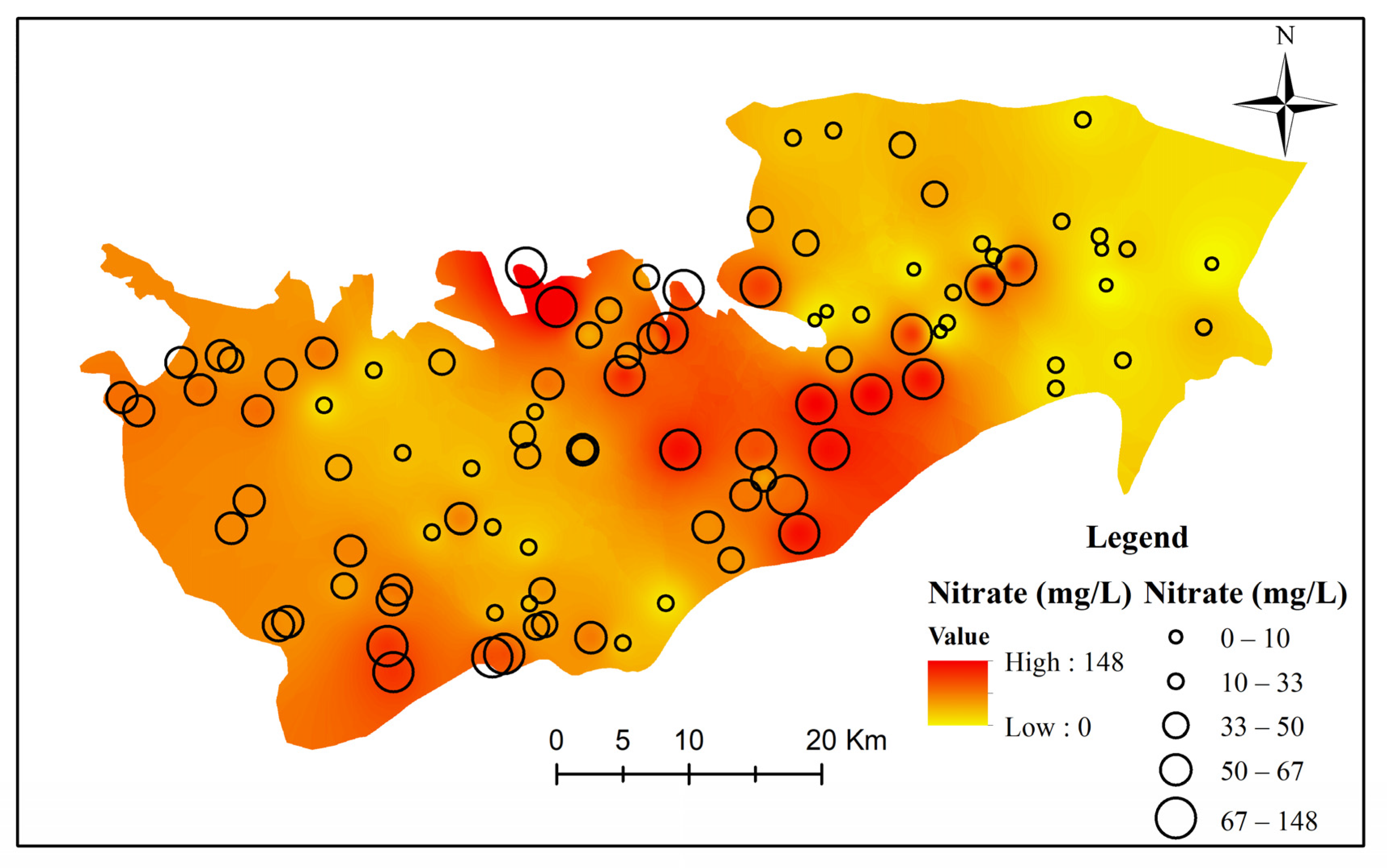
2.4. Preparation of Nitrate Locations’ Data and Validation

In this study, a total of 100 well samples (Figure 3) were selected to collect nitrate concentration. They were taken from the Sebou Hydraulic Basin Agency (SHBA). For the analysis, the inverse distance weighted (IDW) interpolation was performed for the samples. The result of nitrate mapping is presented in Figure 3. Following the recommendations of the WHO, i.e., an aquifer receiving a concentration of nitrate exceeding 50 mg/L is considered polluted. To validate the machine learning models, nitrate concentration data, which served as target in this study, were divided into 2 groups: locations with nitrate concentrations higher than 50 mg/L were classified as polluted areas, whereas those with nitrate concentrations less than 50 mg/L were classified as unpolluted areas. We randomly separated groundwater polluted areas and groundwater unpolluted areas; out of 100 samples of nitrate concentrations, 70% were used as training dataset and 30% were used as validation dataset.

2.5. Algorithm Background and Implementations

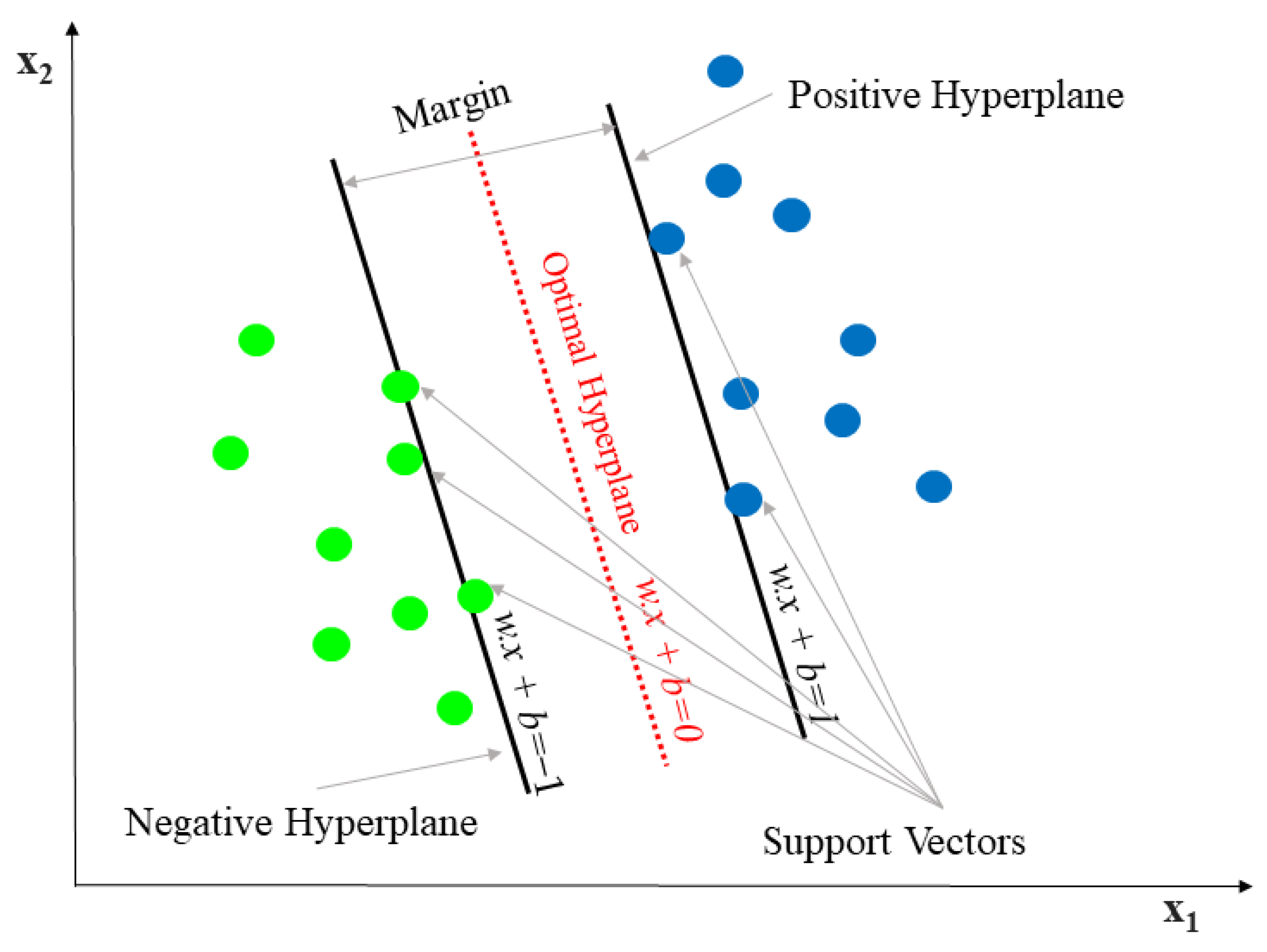
2.5.1. Support Vector Machine (SVM)

SVM was developed for the first time by Vapnik with colleagues [42,43]. It is used for classification and problems. The goal of SVM algorithm is to find a hyperplane in an N-dimensional space (Figure 4). SVM is widely used with successful results in groundwater potential mapping [44,45], landslide mapping [46], and flood susceptibility assessment [47,48]. In this study, the kernel function was used due to its robustness in previous studies [49,50].

2.5.2. Random Forest (RF)

Developed for the first time by Breiman [51], RF is a supervised machine learning algorithm, based on ensemble technique [52], used for both regression and classification tasks [47]. According to Rahmati et al. [6], running the RF algorithm requires two optimized parameters: the number of variables/factors to be used in each tree-building process (mtry) and the number of trees to be built in the forest to run it (ntree).

In this research, the number of trees was considered as 123 with one random division variable, which led to the highest precision.

RF algorithm was used to evaluate many natural environmental hazard studies, because of its reliability and efficiency [29,53]. RF algorithm was used to evaluate many natural environmental hazards studies, such as gully erosion modelling [54], forest fire mapping [53], and flood susceptibility prediction [55,56].

2.5.3. Multilayer Perceptron-Neural Network (MLP-NN)

Multilayer Perceptron-Neural network MLP-NN is a class of Neural Networks algorithms (ANN) with a structure similar to biological neurons. The structure of MLP-NN models consists of three layers: an input layer, an output layer, and a hidden layer [57,58]. The input layers represent the factors conditioning the risk of pollution, the output layers are considered as classified results that infer the classes of pollution or non-pollution by nitrates, whereas the hidden layer is located between these two, in which the function applies weights. Meanwhile, the hidden layers perform non-linear transformations by applying weights to the inputs and directing them through an activation function as output. The training of this algorithm takes place in three steps: feedforward, backpropagation, and weight adjustment [59,60].

In the current study, in order to achieve the highest performance and to avoid the overfitting problem, two hidden layers were used with 37 neurons in each layer, the Linear Unit Rectification (Relu) was used as activation function, and the optimizer was set to Adam, which was developed by Kingma and Ba [61].

2.6. Validation of Groundwater Vulnerability Models

Evaluating the performance of machine learning models is a mandatory step in the modeling research [52,62]. Common statistical approaches were used by several researchers in related studies [15,55].

In this article, using the training and validation datasets, the receiver operating curve (ROC) was applied to evaluate the performance of the groundwater pollution risk models developed in this study. The ROC is a graphical presentation in which the specificity is plotted on the X-axis and the sensitivity is plotted on the Y-axis at different cut-off thresholds classifications [15,63]. To quantitatively validate the models, the area under the curve (AUC) is often used. It is defined as “the probability of a classifier to correctly anticipate the occurrence or non-occurrence of predefined events”.

In addition, other statistical measures were used, including Sensitivity, Specificity, Accuracy (ACC), and Precision:

$$\mathrm{Accuarcy}=\frac{\mathrm{TP}+\mathrm{TN}}{\mathrm{TP}+\mathrm{TN}+\mathrm{FP}+\mathrm{FN}},$$

(6)

$$\mathrm{Sensitivity}=\frac{\mathrm{TP}}{\mathrm{TP}+\mathrm{FN}},$$

(7)

$$\mathrm{Specificity}=\frac{\mathrm{TN}}{\mathrm{TN}+\mathrm{FP}},$$

(8)

$$\mathrm{Precision}=\frac{\mathrm{TP}}{\mathrm{TP}+\mathrm{FP}},$$

(9)

where FP (false positive) is the number of groundwater points incorrectly predicted and considered as polluted and FN (false negative) is the number of groundwater points considered and predicted as non-polluted; TP (true positive) is the number of nitrate pollution samples classified correctly; and TN (true negative) is the number of non-pollution samples classified correctly.

According to Pham et al. [64], to measure the quality of the model, a threshold classification can be applied to classify the area under the ROC curve (AUC) into five classes, including: values ranging from 0.5 to 0.6, indicating that the prediction of the model is poor, 0.6 to 0.7, indicating a fair quality of prediction, 0.7 to 0.8, indicating a good quality of prediction, 0.8 to 0.9, indicating a very good quality of prediction, and 0.9 to 1, indicating an excellent quality of prediction.

3. Results

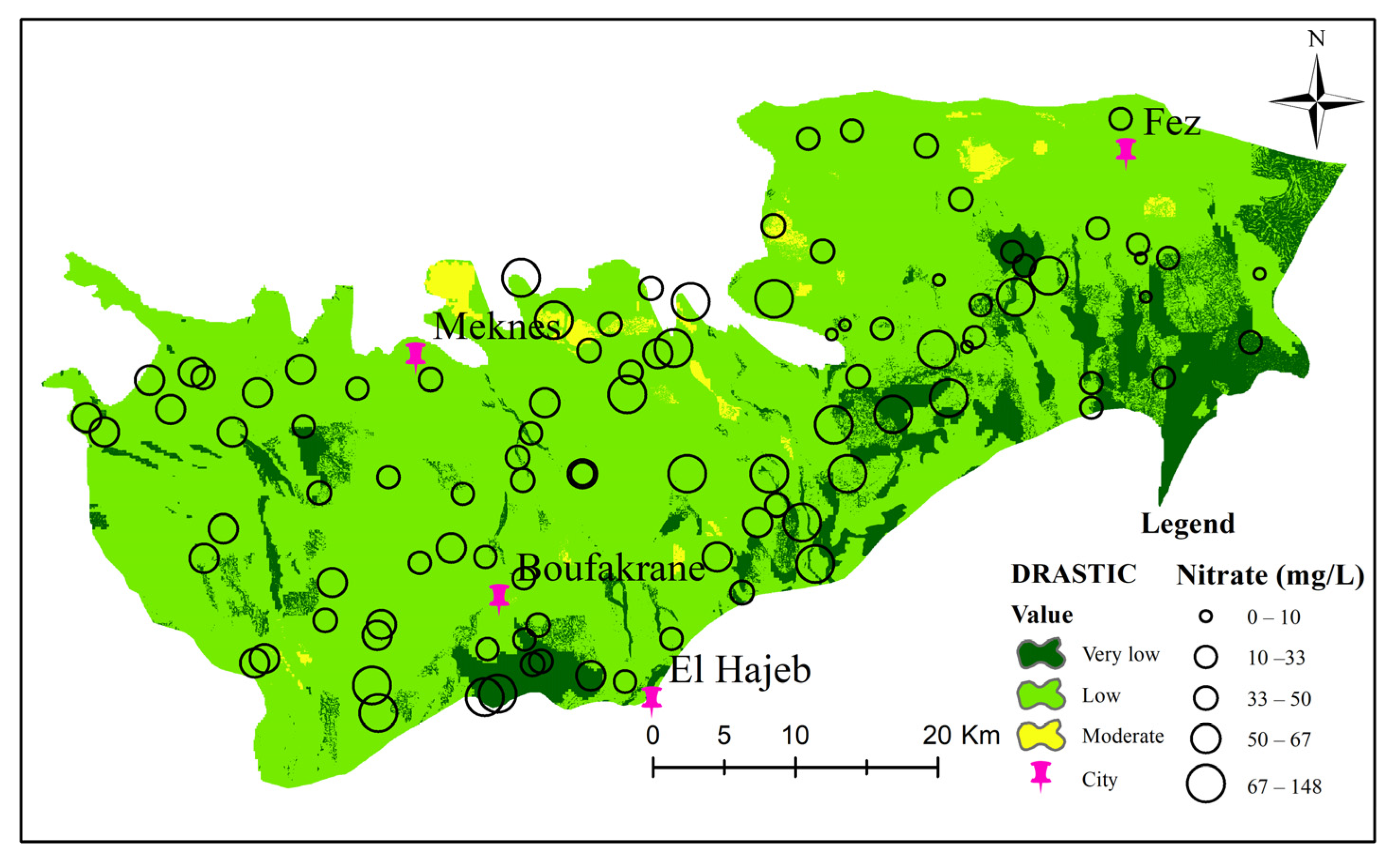
3.1. DRASTIC Vulnerability

After multiplying each of the seven DRASTIC index maps by their standard ratings and weights, the overlays of these seven parameters of the DRASTIC index using Equation (1) were observed to range from 53 to 143.

Following the classification provided by Aller et al. [16], the generated map was divided into three classes of groundwater vulnerability, including very low (14%), low (83%), and medium (3%) (Figure 5).

It can be seen from Figure 5 that the least vulnerable areas are located in the eastern part of the study area. Whereas the south and the west parts of the study area were considered to be without risk, probably due to the high depth (>15) and clay soil, the northeast and the center parts of the basin were considered to be the most vulnerable areas. Due to the low slope (0–12), low depth (0–4.5 m), and high hydraulic conductivity (12–41 m/day), the vadose zone in this area is represented by sandstone and conglomerate.

3.2. Frequency Ratio

Using the frequency ratio bivariate statistic test, the correlations between groundwater pollution risk and each DRASTIC parameter were calculated. As can be seen from Table 1, the net recharge class, ranging from 50 to 100 mm, has the highest FR (0.88). The classes 0–1.5 and 1.5–4.5 of depth to water table and the class 29–41 of hydraulic conductivity present the FR value of zero, i.e., no probability of groundwater pollution with nitrate.

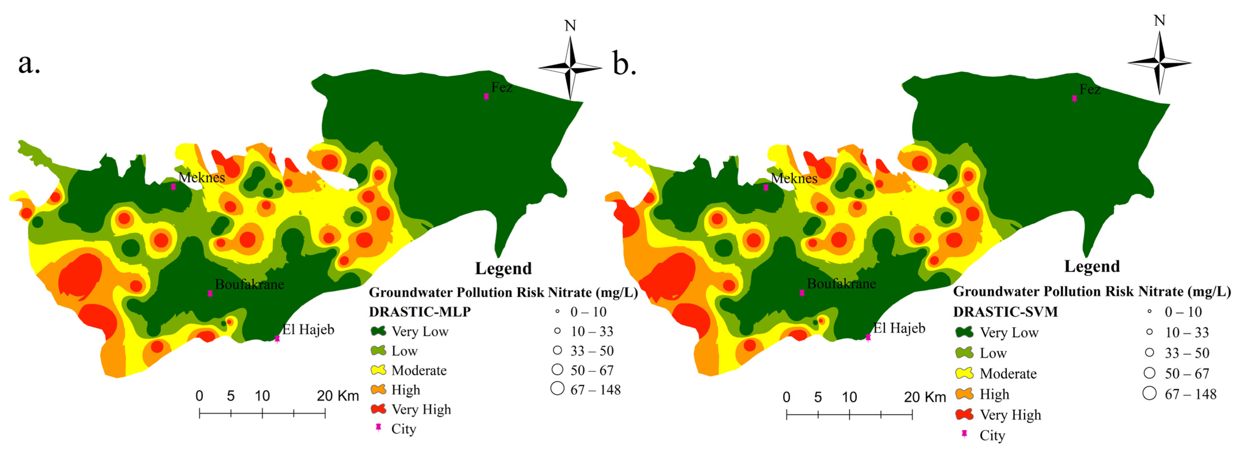
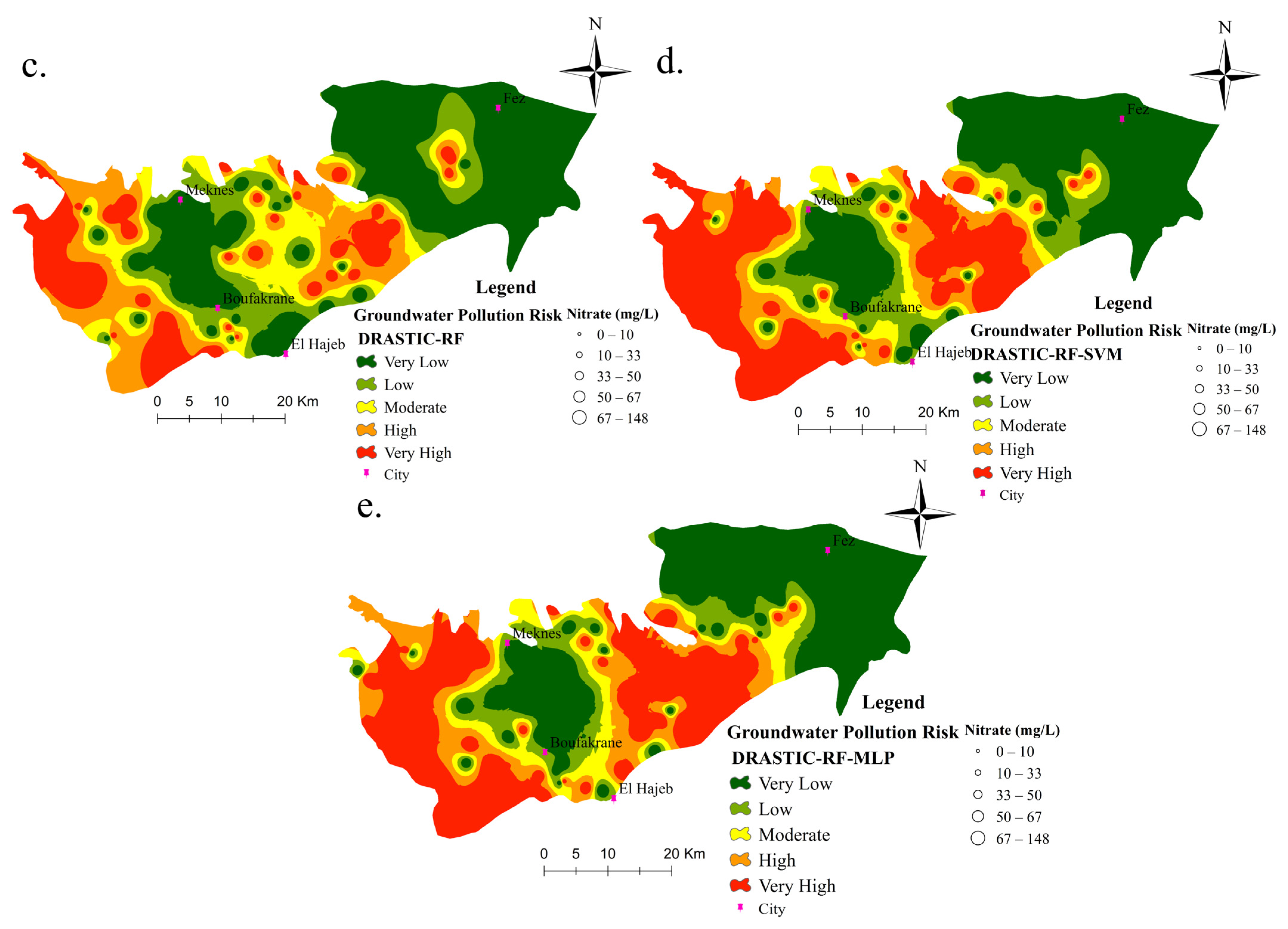
3.3. Groundwater Pollution Risk Maps

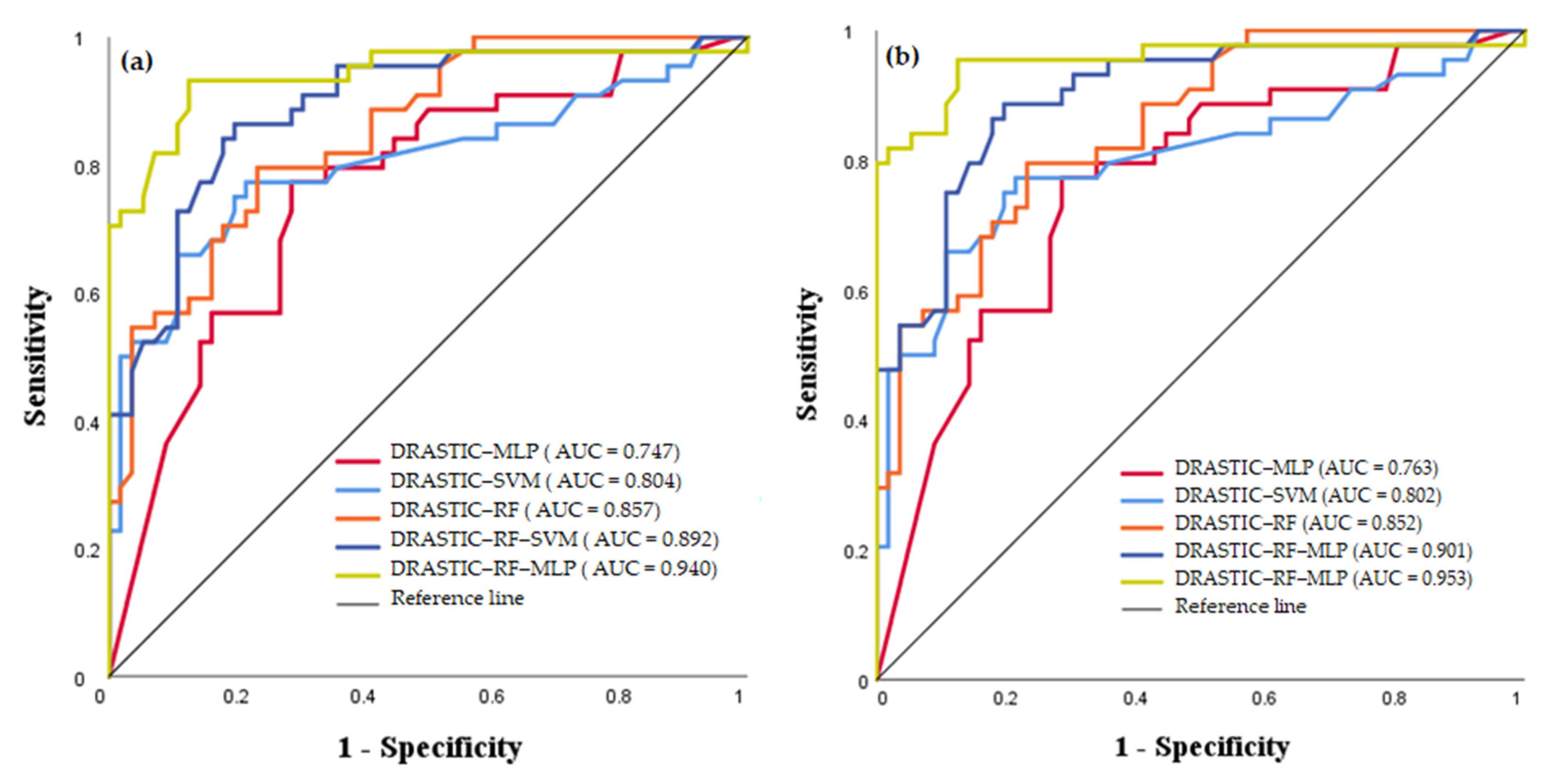
The spatial distribution of groundwater pollution risk maps (GPRMs) for the study area were produced by the DRASTIC method and the applied machine learning models. Using equal interval reclassification within the ArcGIS environment, the generated maps were categorized into five different classes, including very high, high, moderate, low, and very low (Figure 6 and Figure 7).

It can clearly be seen from Figure 7 that the west and the center parts of the basin are at risk of being more contaminated, whereas the eastern part is considered an unpolluted area. For the DRASTIC-MLP model, the pollution risk map (GPRM) elaborated showed that 53% of the basin was characterized as having very low vulnerability risk. Whereas low, medium, high, and very high contributed 15%, 15%, 12%, and 6%, respectively (Figure 7a). For the DRASTIC-SVM model, the GPRM elaborated showed that 52% of the basin was characterized as having very low vulnerability risk. Whereas low, medium, high, and very high contributed 13%, 15%, 12%, and 7%, respectively (Figure 7b). As can be seen from Figure 7c, the generated groundwater pollution risk map (GPRM) produced by RF model showed that 41% of the study area was classified as very low vulnerability, followed by the class of low vulnerability (15%). Whereas medium, high, and very high contributed 13%, 17%, and 14%, respectively. The GPRM generated by the DRASTIC-FR-SVM was divided into five classes: very low vulnerability (38%), low vulnerability (12%), moderate vulnerability (9%), high vulnerability (11%), and very high vulnerability (30%) (Figure 7d). The GPRM generated by the DRASTIC-FR-MLP was divided into five classes: very low vulnerability (36%), low vulnerability (10%), moderate vulnerability (9%), high vulnerability (15%), and very high vulnerability (30%) (Figure 7e).

3.4. Validation

Using the training and the validation datasets, the performance of the developed models in this study was evaluated. The DRASTIC-RF-MLP ensemble outperformed all other models developed in this study. Thus, based on the training dataset (

Table 2. Model statistical measures assigned to training and validation datasets.

Models	Sample	Accuracy	Precision	Sensitivity	Specificity
DRASTIC-SVM	Training	0.743	0.718	0.800	0.686
	Validation	0.733	0.706	0.800	0.667
DRASTIC-MLP	Training	0.786	0.750	0.857	0.733
	Validation	0.767	0.750	0.800	0.681
DRASTIC-RF	Training	0.886	0.865	0.914	0.875
	Validation	0.871	0.857	0.875	0.867
DRASTIC-RF-SVM	Training	0.914	0.892	0.943	0.886
	Validation	0.900	0.933	0.875	0.929
DRASTIC-RF-MLP	Training	0.957	0.943	0.971	0.944
	Validation	0.952	0.969	0.939	0.966

), the following values were obtained: Accuracy = 0.957, Precision = 0.943, Sensitivity = 0.971, and Specificity = 0.944. Based on the validation dataset, the following statistical values were obtained: Accuracy = 0.7952, Precision = 0.969, Sensitivity = 0.939, and Specificity = 0.966.

The DRASTIC-RF-SVM ensemble performed second best, with the training dataset revealing the following values shown in Table 2: Accuracy = 0.914, Precision = 0.892, Sensitivity = 0.943, and Specificity = 0.886; whereas the implication of the validation dataset yields the following statistical values: Accuracy = 0.900, Precision = 0.933, Sensitivity = 0.875, and Specificity = 0.929.

Based on the training dataset, the performances obtained by the DRASTIC-RF model revealed: Accuracy = 0.886, Precision = 0.865, Sensitivity = 0.914, and Specificity = 0.875 (Table 2). Thus, for the validation dataset: Accuracy= 0.871, Precision= 0.857, Sensitivity = 0.875, and Specificity = 0.867.

The performances obtained by the DRASTIC-SVM ensemble were as follows for the training dataset (Table 2): Accuracy (0.743), Precision (0.718), Sensitivity (0.840), and Specificity (0.686). Thus, the validation dataset achieved the following statistical values: Accuracy (0.733), Precision (0.706), Sensitivity (0.800), and Specificity (0.667). The DRASTIC-MLP model has the lowest performance in comparison to the other developed models. Thus, for the training dataset, as shown in Table 2, the following statistical values were obtained: Accuracy (0.786), Precision (0.750), Sensitivity (0.857), and Specificity (0.733). For the validation dataset, our results show: Accuracy (0.767), Precision (0. 750), Sensitivity (0.800), and Specificity (0.681).

The AUC value of the original DRASTIC method was equal to 0.53. However, the applied machine learning models, including DRASTIC-MLP, DRASTIC-SVM, DRASTIC-RF, DRASTIC-RF-SVM, and DRASTIC-RF-MLP performed better with AUC values of 0.747, 0.804, 0.857, 0.892, and 0.940, respectively, in term of Success Rate (Figure 8a). In addition, based on the prediction rate (Figure 8b), the AUCs values were as follows: 0.763, 0.803, 0.852, 0.901, and 0.953 for DRASTIC-MLP, DRASTIC-SVM, DRASTIC-RF, DRASTIC-RF-SVM, and DRASTIC-RF-MLP, respectively. It should be noted that the DRASTIC-RF-MLP ensemble model had the highest performance. Our results indicate that both in terms of success and prediction rate, the use of machine learning algorithms improves the performance of the DRASTIC method.

3.5. Variable Importance

In all modeling research purposes, variables’ importance should be applied to find the suitable predictive variables for the modelling research [65,66]. In this study, the RF model was used to evaluate the importance of the DRASTIC parameters. Our findings showed that both the depth of groundwater (1.8) and the hydraulic conductivity (1.6) had the highest importance in groundwater vulnerability assessment, followed by net recharge (1.49), aquifer media (1.38), topography (1.27), soil (1.21), and the impact of the vadose zone (0.97).

4. Discussion

Groundwater pollution is one of the challenging issues in the world, especially in arid and semi-arid ecosystems [20]. To overcome this issue, researchers have deployed great efforts to prevent and manage water contamination. The DRASTIC method is a widely applied approach to assess groundwater pollution.

Our results showed that the north and central parts tended to have a moderate risk of pollution, whereas the least vulnerable areas are located in the eastern parts of the study area. The south and west parts of the study area are considered to be without risk. This could be due to the hydrological background of the study area (i.e., low slope, lowest depth, highest hydraulic conductivity, and the lithological nature) [67]. Similar to our results, previous research reported that a higher groundwater vulnerability was observed in downslope areas [68], meaning the higher the hydraulic conductivity, the higher the risk of groundwater [67]. According to Baghapour et al. [68], the slope has an important impact. In addition, [21] indicated that the lowest depth is more affected by groundwater vulnerability.

Due to its uncertainty, many researchers have modified the original DRASTIC method using statistical techniques and machine learning models to increase its accuracy. In this study, five new individual models and their ensemble machine learning models were developed, namely DRASTIC-RF, DRASTIC-SVM, DRASTIC-MLP, DRASTIC-RF-SVM, and DRASTIC-RF-MLP, for groundwater pollution risk assessment in the Saiss basin, in Morocco.

Through its ability to handle large datasets, its low aptitude to overfitting, and its ability to learn non-linear relationships between the nitrate polluted samples and the input layers [15], random forest has shown greater accuracy in previous studies [26,53]. In addition, Ref. [44] confirms that RF is one of the successful machine learning models for groundwater mapping.

Hybrid/ensemble approaches have been proposed recently to improve the performance of both individual machine learning models and bivariate statistical techniques [24,42,51]. In the current research, RF was used to improve the accuracy of the other applied models. In term of the accuracy, our results show that the DRASTIC-RF-MLP hybrid model provided the best accuracy in comparison to the other models. MLP has been used in several studies with successful results because of its ability to deal with complex non-linear problems and ease in processing large numbers of input data [24].

In terms of the DRASTIC-RF-SVM model, the SVM algorithm has significant advantages in solving linear and non-linear problems and works well in high dimensional spaces [48]. It has already revealed great potential for groundwater mapping [45,52].

It should be highlighted that selecting the best model is not an easy task because all the aforementioned models present their own advantages and drawbacks. In addition, we can add that the outcomes of this research are limited and related to the study area background and the data used. Thus, it can be concluded that all the above discussed models can be used for any hazard environment monitoring studies, including groundwater pollution risk mapping, for other environment backgrounds with promising results.

Our findings showed that both depth of groundwater and hydraulic conductivity had the highest importance in groundwater vulnerability assessment, followed by net recharge, aquifer media, topography, soil, and impact of the vadose zone. Similar findings were also found by [52,69]. From our results, depth of groundwater is the most important variable; this is because the groundwater could easily be contaminated by surface runoff and contaminants. These findings agree with Pham et al. [52], who also confirm that depth of groundwater is the most significant factor for groundwater potential mapping. Hydraulic conductivity is considered an important factor for groundwater management strategies because it controls the contaminants’ migration rate from the source to the aquifer.

With the rapid population growth in the Fes-Meknes region, urbanization and extensive use of soils for agriculture activities have become serious challenges for environmental agency, leading to the groundwater quality deterioration in the Saiss basin. In the same geographical area, in a recent work El Hafyani et al. [70] reported that the increase in water consumption is linked to Meknes city’s urban growth and the agricultural activities’ system adopted. In addition, the impact of climate change on natural resources has been investigated in this study area [71]. Laraichi et al. [72] demonstrated a weakening in the transmission of information and communication about groundwater, which might lead to several issues including overexploitation and pollution. For instance, Benaabidate et al. [73] reported in their study a decrease in piezometric level, which is mainly due to several factors, including the decrease in precipitation, the reduced natural aquifer recharge, and the increased pumping, mainly for irrigation. Likewise, a recent work by Berni et al. [9] highlighted that a negative effect of pesticides in the Saiss basin was explained by farmers’ safety behavior. Additionally, expert interpretations confirmed that a clear link between groundwater vulnerability risk and geological background of the Saiss basin was shown, highlighting that Meknes city is more susceptible to groundwater pollution, which is probably due to the existence of permeable Paleocene sands in this area.

Our results indicate that the most vulnerable areas are located in the northeast and the center of the basin, because of low depth, low slope, high recharge, and high hydraulic conductivity, whereas the high depth, low recharge, and low conductivity of the western areas of the Saiss cause this part to be considered as without risk. These findings are in line with previous works [9,35]. Thus, the delineation of highly affected areas to pollution is urgently needed to avoid the deterioration of groundwater resources. In this aquifer, as agriculture is still going to be one of the main sources of the local population, to meet the livelihood’s resource requirements, more comprehensive studies should be carried out to promote the sustainable use of natural resources for the proper management and planning of them. Therefore, the proposed methodology could be a newer, effective tool and an emergent path to decision making for assessing groundwater pollution based on the performance accuracy of hybrid machine learning algorithms.

Marking vulnerable areas to pollution based on the opportunities of the developed models will be very helpful in encouraging the ongoing efforts to develop a geoportal platform in the framework of the VLIR-UOS project through a collaborative effort with scientists and different environmental agencies (https://www.vliruos.be/en/projects/project/ (accessed on 14 December 2021).Furthermore, this work contributes to the aim of the Sustainable Development Goals (SDGs) framework on its sixth goal, which is dedicated to water sustainability and different indicators related to water quality.

5. Conclusions

In this study, five new hybrid models were developed based on the modified DRASTIC method by the frequency ration bivariate statistic test and the random forest machine learning algorithm, namely DRASTIC-RF, DRASTIC-SVM, DRASTIC-MLP, DRASTIC-RF-SVM, and DRASTIC-RF-MLP, for groundwater pollution assessment in the Saiss basin. Furthermore, three conclusions can be highlighted.

-

The results obtained indicate that the most vulnerable areas are located in the west and the center parts of the basin, because of the low depth, low slope, and high hydraulic conductivity, whereas the high depth, low recharge, and low conductivity of the western areas of the Saiss basin mean that this area is considered to be without risk;

-

As expected, the locations subject to high vulnerability risk are associated with a high concentration of nitrate;

-

The spatial distribution of groundwater pollution risk maps (GPRMs) for the study area show that the west and the center parts of the basin are the most vulnerable areas;

-

The results highlight that the hybrid/ensemble machine learning (ML) model outperforms the individual based model.

It should be noted that the overall goal beyond this research is to implement a machine learning algorithm to understand groundwater pollution. Furthermore, the output will help the authorities and government agencies in designing appropriate decision-making strategies.

Finally, in a vision to protect our environment, the methodology developed here could be applied in other case studies with similar background.

References

1. Jesiya, N.P.; Gopinath, G. A Fuzzy Based MCDM–GIS Framework to Evaluate Groundwater Potential Index for Sustainable Groundwater Management—A Case Study in an Urban-Periurban Ensemble, Southern India. Groundw. Sustain. Dev. 2020, 11, 100466. [Google Scholar] [CrossRef]
2. Naghibi, S.A.; Pourghasemi, H.R.; Dixon, B. GIS-Based Groundwater Potential Mapping Using Boosted Regression Tree, Classification and Regression Tree, and Random Forest Machine Learning Models in Iran. Environ. Monit. Assess. 2016, 188, 44. [Google Scholar] [CrossRef] [PubMed]
3. Organisation Mondiale de la Santé; UNICEF. Progress on Drinking Water, Sanitation and Hygiene: 2017 Update and SDG Baselines; World Health Organization: Geneva, Switzerland, 2017; ISBN 978-92-4-151289-3. [Google Scholar]
4. Omarova, A.; Tussupova, K.; Hjorth, P.; Kalishev, M.; Dosmagambetova, R. Water Supply Challenges in Rural Areas: A Case Study from Central Kazakhstan. Int. J. Environ. Res. Public. Health 2019, 16, 688. [Google Scholar] [CrossRef] [PubMed] [Green Version]
5. Kammoun, S.; Trabelsi, R.; Re, V.; Zouari, K.; Henchiri, J. Groundwater Quality Assessment in Semi-Arid Regions Using Integrated Approaches: The Case of Grombalia Aquifer (NE Tunisia). Environ. Monit. Assess. 2018, 190, 87. [Google Scholar] [CrossRef] [PubMed]
6. Rahmati, O.; Melesse, A.M. Application of Dempster–Shafer Theory, Spatial Analysis and Remote Sensing for Groundwater Potentiality and Nitrate Pollution Analysis in the Semi-Arid Region of Khuzestan, Iran. Sci. Total Environ. 2016, 568, 1110–1123. [Google Scholar] [CrossRef] [PubMed]
7. Chen, R.; Teng, Y.; Chen, H.; Hu, B.; Yue, W. Groundwater Pollution and Risk Assessment Based on Source Apportionment in a Typical Cold Agricultural Region in Northeastern China. Sci. Total Environ. 2019, 696, 133972. [Google Scholar] [CrossRef] [PubMed]
8. Serio, F.; Miglietta, P.P.; Lamastra, L.; Ficocelli, S.; Intini, F.; De Leo, F.; De Donno, A. Groundwater Nitrate Contamination and Agricultural Land Use: A Grey Water Footprint Perspective in Southern Apulia Region (Italy). Sci. Total Environ. 2018, 645, 1425–1431. [Google Scholar] [CrossRef]
9. Berni, I.; Menouni, A.; El Ghazi, I.; Godderis, L.; Duca, R.-C.; Jaafari, S.E. Health and Ecological Risk Assessment Based on Pesticide Monitoring in Saïss Plain (Morocco) Groundwater. Environ. Pollut. 2021, 276, 116638. [Google Scholar] [CrossRef]
10. Möhring, N.; Dalhaus, T.; Enjolras, G.; Finger, R. Crop Insurance and Pesticide Use in European Agriculture. Agric. Syst. 2020, 184, 102902. [Google Scholar] [CrossRef]
11. Sanchezperez, J.; Antiguedad, I.; Arrate, I.; Garcialinares, C.; Morell, I. The Influence of Nitrate Leaching through Unsaturated Soil on Groundwater Pollution in an Agricultural Area of the Basque Country: A Case Study. Sci. Total Environ. 2003, 317, 173–187. [Google Scholar] [CrossRef] [Green Version]
12. Biddau, R.; Cidu, R.; Da Pelo, S.; Carletti, A.; Ghiglieri, G.; Pittalis, D. Source and Fate of Nitrate in Contaminated Groundwater Systems: Assessing Spatial and Temporal Variations by Hydrogeochemistry and Multiple Stable Isotope Tools. Sci. Total Environ. 2019, 647, 1121–1136. [Google Scholar] [CrossRef] [PubMed]
13. Meng, L.; Zhang, Q.; Liu, P.; He, H.; Xu, W. Influence of Agricultural Irrigation Activity on the Potential Risk of Groundwater Pollution: A Study with Drastic Method in a Semi-Arid Agricultural Region of China. Sustainability 2020, 12, 1954. [Google Scholar] [CrossRef] [Green Version]
14. Oliveira, A.; Lopes, A.; Niza, S. Local Climate Zones in Five Southern European Cities: An Improved GIS-Based Classification Method Based on Copernicus Data. Urban Clim. 2020, 33, 100631. [Google Scholar] [CrossRef]
15. Rodriguez-Galiano, V.; Mendes, M.P.; Garcia-Soldado, M.J.; Chica-Olmo, M.; Ribeiro, L. Predictive Modeling of Groundwater Nitrate Pollution Using Random Forest and Multisource Variables Related to Intrinsic and Specific Vulnerability: A Case Study in an Agricultural Setting (Southern Spain). Sci. Total Environ. 2014, 476–477, 189–206. [Google Scholar] [CrossRef] [PubMed]
16. Aller, L.; Lehr, J.H.; Petty, R.; Bennett, T. DRASTIC: A Standardized System for Evaluating Ground Water Pollution Potential Using Hydrogeologic Settings; Robert, S., Ed.; Kerr Environmental Research Laboratory, Office of Research and Development, U.S. Environmental Protection Agency: Ada, OK, USA, 1987. [Google Scholar]
17. Arya, S.; Subramani, T.; Vennila, G.; Roy, P.D. Groundwater Vulnerability to Pollution in the Semi-Arid Vattamalaikarai River Basin of South India Thorough DRASTIC Index Evaluation. Geochemistry 2020, 80, 125635. [Google Scholar] [CrossRef]
18. Sinan, M.; Razack, M. An Extension to the DRASTIC Model to Assess Groundwater Vulnerability to Pollution: Application to the Haouz Aquifer of Marrakech (Morocco). Environ. Geol. 2009, 57, 349–363. [Google Scholar] [CrossRef]
19. Arshad, A.; Zhang, Z.; Zhang, W.; Dilawar, A. Mapping Favorable Groundwater Potential Recharge Zones Using a GIS-Based Analytical Hierarchical Process and Probability Frequency Ratio Model: A Case Study from an Agro-Urban Region of Pakistan. Geosci. Front. 2020, 11, 1805–1819. [Google Scholar] [CrossRef]
20. Nadiri, A.A.; Sedghi, Z.; Khatibi, R.; Gharekhani, M. Mapping Vulnerability of Multiple Aquifers Using Multiple Models and Fuzzy Logic to Objectively Derive Model Structures. Sci. Total Environ. 2017, 593–594, 75–90. [Google Scholar] [CrossRef]
21. Khosravi, K.; Sartaj, M.; Tsai, F.T.-C.; Singh, V.P.; Kazakis, N.; Melesse, A.M.; Prakash, I.; Tien Bui, D.; Pham, B.T. A Comparison Study of DRASTIC Methods with Various Objective Methods for Groundwater Vulnerability Assessment. Sci. Total Environ. 2018, 642, 1032–1049. [Google Scholar] [CrossRef]
22. Sarkar, T.; Mishra, M. Soil Erosion Susceptibility Mapping with the Application of Logistic Regression and Artificial Neural Network. J. Geovisualization Spat. Anal. 2018, 2, 8. [Google Scholar] [CrossRef]
23. Neshat, A.; Pradhan, B. An Integrated DRASTIC Model Using Frequency Ratio and Two New Hybrid Methods for Groundwater Vulnerability Assessment. Nat. Hazards 2015, 76, 543–563. [Google Scholar] [CrossRef] [Green Version]
24. Fijani, E.; Nadiri, A.A.; Asghari Moghaddam, A.; Tsai, F.T.-C.; Dixon, B. Optimization of DRASTIC Method by Supervised Committee Machine Artificial Intelligence to Assess Groundwater Vulnerability for Maragheh–Bonab Plain Aquifer, Iran. J. Hydrol. 2013, 503, 89–100. [Google Scholar] [CrossRef]
25. Asfaw, D.; Mengistu, D. Modeling Megech Watershed Aquifer Vulnerability to Pollution Using Modified DRASTIC Model for Sustainable Groundwater Management, Northwestern Ethiopia. Groundw. Sustain. Dev. 2020, 11, 100375. [Google Scholar] [CrossRef]
26. Hosseini, F.S.; Choubin, B.; Mosavi, A.; Nabipour, N.; Shamshirband, S.; Darabi, H.; Haghighi, A.T. Flash-Flood Hazard Assessment Using Ensembles and Bayesian-Based Machine Learning Models: Application of the Simulated Annealing Feature Selection Method. Sci. Total Environ. 2020, 711, 135161. [Google Scholar] [CrossRef] [PubMed]
27. Wang, Y.; Feng, L.; Li, S.; Ren, F.; Du, Q. A Hybrid Model Considering Spatial Heterogeneity for Landslide Susceptibility Mapping in Zhejiang Province, China. CATENA 2020, 188, 104425. [Google Scholar] [CrossRef]
28. Chapi, K.; Singh, V.P.; Shirzadi, A.; Shahabi, H.; Bui, D.T.; Pham, B.T.; Khosravi, K. A Novel Hybrid Artificial Intelligence Approach for Flood Susceptibility Assessment. Environ. Model. Softw. 2017, 95, 229–245. [Google Scholar] [CrossRef]
29. Costache, R. Flash-Flood Potential Assessment in the Upper and Middle Sector of Prahova River Catchment (Romania). A Comparative Approach between Four Hybrid Models. Sci. Total Environ. 2019, 659, 1115–1134. [Google Scholar] [CrossRef]
30. Pham, B.T.; Prakash, I.; Singh, S.K.; Shirzadi, A.; Shahabi, H.; Tran, T.-T.-T.; Bui, D.T. Landslide Susceptibility Modeling Using Reduced Error Pruning Trees and Different Ensemble Techniques: Hybrid Machine Learning Approaches. CATENA 2019, 175, 203–218. [Google Scholar] [CrossRef]
31. Pham, B.T.; Tien Bui, D.; Prakash, I.; Dholakia, M.B. Hybrid Integration of Multilayer Perceptron Neural Networks and Machine Learning Ensembles for Landslide Susceptibility Assessment at Himalayan Area (India) Using GIS. CATENA 2017, 149, 52–63. [Google Scholar] [CrossRef]
32. Tien Bui, D.; Bui, Q.-T.; Nguyen, Q.-P.; Pradhan, B.; Nampak, H.; Trinh, P.T. A Hybrid Artificial Intelligence Approach Using GIS-Based Neural-Fuzzy Inference System and Particle Swarm Optimization for Forest Fire Susceptibility Modeling at a Tropical Area. Agric. For. Meteorol. 2017, 233, 32–44. [Google Scholar] [CrossRef]
33. Yadav, B.; Gupta, P.K.; Patidar, N.; Himanshu, S.K. Ensemble Modelling Framework for Groundwater Level Prediction in Urban Areas of India. Sci. Total Environ. 2020, 712, 135539. [Google Scholar] [CrossRef] [PubMed]
34. Sadkaoui, N.; Boukrim, S.; Bourak, A.; Lakhili, F.; Mesrar, L.; Chaouni, A.-A.; Lahrach, A.; Jabrane, R.; Akdim, B. Groundwater pollution of SAÏS basin (Morocco), vulnerability mapping by drastic, god and PRK methods, involving geographic information system (GIS). Present Environ. Sustain. Dev. 2013, 7, 298–308. [Google Scholar]
35. Lahjouj, A.; El Hmaidi, A.; Bouhafa, K.; Boufala, M. Mapping Specific Groundwater Vulnerability to Nitrate Using Random Forest: Case of Sais Basin, Morocco. Model. Earth Syst. Environ. 2020, 6, 1451–1466. [Google Scholar] [CrossRef]
36. Margat, J. Hydrogeological Map of the Meknes-Fes Basin; Edition of the Office of Irrigation: Rabat, Morocco, 1960. [Google Scholar]
37. Essahlaoui, A.; Sahbi, H.; Bahi, L.; El-Yamine, N. Reconnaissance de la structure géologique du bassin de saïss occidental, Maroc, par sondages électriques. J. Afr. Earth Sci. 2001, 32, 777–789. [Google Scholar] [CrossRef]
38. Scanlon, B.R.; Healy, R.W.; Cook, P.G. Choosing Appropriate Techniques for Quantifying Groundwater Recharge. Hydrogeol. J. 2002, 10, 18–39. [Google Scholar] [CrossRef]
39. Khosravi, K.; Sartaj, M.; Karimi, M.; Levison, J.; Lotfi, A. A GIS-Based Groundwater Pollution Potential Using DRASTIC, Modified DRASTIC, and Bivariate Statistical Models. Environ. Sci. Pollut. Res. 2021, 28, 50525–50541. [Google Scholar] [CrossRef]
40. Tehrany, M.S.; Jones, S.; Shabani, F.; Martínez-Álvarez, F.; Tien Bui, D. A Novel Ensemble Modeling Approach for the Spatial Prediction of Tropical Forest Fire Susceptibility Using LogitBoost Machine Learning Classifier and Multi-Source Geospatial Data. Theor. Appl. Climatol. 2019, 137, 637–653. [Google Scholar] [CrossRef]
41. Pradhan, B.; Lee, S. Landslide Risk Analysis Using Artificial Neural Network Model Focussing on Different Training Sites. Int. J. Phys. Sci. 2009, 4, 1–15. [Google Scholar]
42. Guyon, I.; Weston, J.; Barnhill, S. Gene selection for cancer classification using support vector machines. Mach. Learn. 2002, 46, 389–422. [Google Scholar] [CrossRef]
43. Boser, B.E.; Guyon, I.M.; Vapnik, V.N. A Training Algorithm for Optimal Margin Classifiers | Proceedings of the Fifth Annual Workshop on Computational Learning Theory. Available online: https://dl.acm.org/doi/abs/10.1145/130385.130401 (accessed on 6 May 2022).
44. Naghibi, S.A.; Ahmadi, K.; Daneshi, A. Application of Support Vector Machine, Random Forest, and Genetic Algorithm Optimized Random Forest Models in Groundwater Potential Mapping. Water Resour. Manag. 2017, 31, 2761–2775. [Google Scholar] [CrossRef]
45. Yousefi, S.; Sadhasivam, N.; Pourghasemi, H.R.; Ghaffari Nazarlou, H.; Golkar, F.; Tavangar, S.; Santosh, M. Groundwater Spring Potential Assessment Using New Ensemble Data Mining Techniques. Measurement 2020, 157, 107652. [Google Scholar] [CrossRef]
46. Han, H.; Shi, B.; Zhang, L. Prediction of Landslide Sharp Increase Displacement by SVM with Considering Hysteresis of Groundwater Change. Eng. Geol. 2021, 280, 105876. [Google Scholar] [CrossRef]
47. Costache, R.; Hong, H.; Pham, Q.B. Comparative Assessment of the Flash-Flood Potential within Small Mountain Catchments Using Bivariate Statistics and Their Novel Hybrid Integration with Machine Learning Models. Sci. Total Environ. 2020, 711, 134514. [Google Scholar] [CrossRef] [PubMed]
48. Tehrany, M.S.; Pradhan, B.; Jebur, M.N. Flood Susceptibility Analysis and Its Verification Using a Novel Ensemble Support Vector Machine and Frequency Ratio Method. Stoch. Environ. Res. Risk Assess. 2015, 29, 1149–1165. [Google Scholar] [CrossRef]
49. Kavzoglu, T.; Colkesen, I. A Kernel Functions Analysis for Support Vector Machines for Land Cover Classification. Int. J. Appl. Earth Obs. Geoinf. 2009, 11, 352–359. [Google Scholar] [CrossRef]
50. Pourghasemi, H.R.; Jirandeh, A.G.; Pradhan, B.; Xu, C.; Gokceoglu, C. Landslide Susceptibility Mapping Using Support Vector Machine and GIS at the Golestan Province, Iran. J. Earth Syst. Sci. 2013, 122, 349–369. [Google Scholar] [CrossRef] [Green Version]
51. Breiman, L. Random Forests. Mach. Learn. 2001, 45, 5–32. Available online: https://link.springer.com/article/10.1023/A:1010933404324 (accessed on 17 April 2021). [CrossRef] [Green Version]
52. Rahmati, O.; Choubin, B.; Fathabadi, A.; Coulon, F.; Soltani, E.; Shahabi, H.; Mollaefar, E.; Tiefenbacher, J.; Cipullo, S.; Ahmad, B.B.; et al. Predicting Uncertainty of Machine Learning Models for Modelling Nitrate Pollution of Groundwater Using Quantile Regression and UNEEC Methods. Sci. Total Environ. 2019, 688, 855–866. [Google Scholar] [CrossRef]
53. Mohajane, M.; Costache, R.; Karimi, F.; Bao Pham, Q.; Essahlaoui, A.; Nguyen, H.; Laneve, G.; Oudija, F. Application of Remote Sensing and Machine Learning Algorithms for Forest Fire Mapping in a Mediterranean Area. Ecol. Indic. 2021, 129, 107869. [Google Scholar] [CrossRef]
54. Jiang, T.; Gradus, J.L.; Lash, T.L.; Fox, M.P. Addressing Measurement Error in Random Forests Using Quantitative Bias Analysis. Am. J. Epidemiol. 2021, 190, 1830–1840. [Google Scholar] [CrossRef]
55. Chen, W.; Li, Y.; Xue, W.; Shahabi, H.; Li, S.; Hong, H.; Wang, X.; Bian, H.; Zhang, S.; Pradhan, B.; et al. Modeling Flood Susceptibility Using Data-Driven Approaches of Naïve Bayes Tree, Alternating Decision Tree, and Random Forest Methods. Sci. Total Environ. 2020, 701, 134979. [Google Scholar] [CrossRef] [PubMed]
56. Schoppa, L.; Disse, M.; Bachmair, S. Evaluating the Performance of Random Forest for Large-Scale Flood Discharge Simulation. J. Hydrol. 2020, 590, 125531. [Google Scholar] [CrossRef]
57. Kavzoglu, T.; Mather, P.M. The Use of Backpropagating Artificial Neural Networks in Land Cover Classification. Int. J. Remote Sens. 2003, 24, 4907–4938. [Google Scholar] [CrossRef]
58. Rosenblatt, F. The Perceptron: A Probabilistic Model for Information Storage and Organization in the Brain. Psychol. Rev. 1958, 65, 386–408. [Google Scholar] [CrossRef] [PubMed] [Green Version]
59. Basheer, I.A.; Hajmeer, M. Artificial Neural Networks: Fundamentals, Computing, Design, and Application. J. Microbiol. Methods 2000, 43, 3–31. [Google Scholar] [CrossRef]
60. Fausett, L. Fundamentals Of Neural Networks: Architectures, Algorithms, and Applications; Prenctice-Hall: Hoboken, NJ, USA, 1994. [Google Scholar]
61. Kingma, D.P.; Ba, J. Adam: A Method for Stochastic Optimization. arXiv 2017, arXiv:1412.6980. [Google Scholar]
62. Yen, H.P.H.; Pham, B.T.; Phong, T.V.; Ha, D.H.; Costache, R.; Le, H.V.; Nguyen, H.D.; Amiri, M.; Tao, N.V.; Prakash, I. Locally Weighted Learning Based Hybrid Intelligence Models for Groundwater Potential Mapping and Modeling: A Case Study at Gia Lai Province, Vietnam. Geosci. Front. 2021, 12, 101154. [Google Scholar] [CrossRef]
63. Costache, R.; Bui, D.T. Spatial prediction of flood potential using new ensembles of bivariate statistics and artificial intelligence: A case study at the Putna river catchment of Romania. Sci. Total Environ. 2019, 691, 1098–1118. [Google Scholar] [CrossRef]
64. Pham, B.T.; Jaafari, A.; Prakash, I.; Singh, S.K.; Quoc, N.K.; Bui, D.T. Hybrid Computational Intelligence Models for Groundwater Potential Mapping. CATENA 2019, 182, 104101. [Google Scholar] [CrossRef]
65. Costache, R.; Popa, M.C.; Tien Bui, D.; Diaconu, D.C.; Ciubotaru, N.; Minea, G.; Pham, Q.B. Spatial Predicting of Flood Potential Areas Using Novel Hybridizations of Fuzzy Decision-Making, Bivariate Statistics, and Machine Learning. J. Hydrol. 2020, 585, 124808. [Google Scholar] [CrossRef]
66. Hong, H.; Pourghasemi, H.R.; Pourtaghi, Z.S. Landslide Susceptibility Assessment in Lianhua County (China): A Comparison between a Random Forest Data Mining Technique and Bivariate and Multivariate Statistical Models. Geomorphology 2016, 259, 105–118. [Google Scholar] [CrossRef]
67. Bera, A.; Mukhopadhyay, B.P.; Chowdhury, P.; Ghosh, A.; Biswas, S. Groundwater Vulnerability Assessment Using GIS-Based DRASTIC Model in Nangasai River Basin, India with Special Emphasis on Agricultural Contamination. Ecotoxicol. Environ. Saf. 2021, 214, 112085. [Google Scholar] [CrossRef] [PubMed]
68. Baghapour, M.A.; Fadaei Nobandegani, A.; Talebbeydokhti, N.; Bagherzadeh, S.; Nadiri, A.A.; Gharekhani, M.; Chitsazan, N. Optimization of DRASTIC Method by Artificial Neural Network, Nitrate Vulnerability Index, and Composite DRASTIC Models to Assess Groundwater Vulnerability for Unconfined Aquifer of Shiraz Plain, Iran. J. Environ. Health Sci. Eng. 2016, 14, 13. [Google Scholar] [CrossRef] [Green Version]
69. Knoll, L.; Breuer, L.; Bach, M. Large Scale Prediction of Groundwater Nitrate Concentrations from Spatial Data Using Machine Learning. Sci. Total Environ. 2019, 668, 1317–1327. [Google Scholar] [CrossRef] [PubMed]
70. El Hafyani, M.; Essahlaoui, A.; Van Rompaey, A.; Mohajane, M.; El Hmaidi, A.; El Ouali, A.; Moudden, F.; Serrhini, N.-E. Assessing Regional Scale Water Balances through Remote Sensing Techniques: A Case Study of Boufakrane River Watershed, Meknes Region, Morocco. Water 2020, 12, 320. [Google Scholar] [CrossRef] [Green Version]
71. Brouziyne, Y.; Abouabdillah, A.; Bouabid, R.; Benaabidate, L. SWAT Streamflow Modeling for Hydrological Components’ Understanding within an Agro—Sylvo—Pastoral Watershed in Morocco. J. Mater. Environ. Sci. 2018, 9, 128–138. [Google Scholar] [CrossRef]
72. Laraichi, S.; Hammani, A. How Can Information and Communication Effects on Small Farmers’ Engagement in Groundwater Management: Case of SAISS Aquifers, Morocco. Groundw. Sustain. Dev. 2018, 7, 109–120. [Google Scholar] [CrossRef]
73. Benaabidate, L.; Cholli, M. Groundwater stress and vulnerability to pollution of SAISS basin shallow aquifer, Morocco. In Proceedings of the Fifteenth International Water Technology Conference, Alexandria, Egypt, 28–30 May 2011. [Google Scholar]
Figure 1. Location and geological map of the Saiss basin, (a) location of the study area, Fes-Meknes region, Morocco. (b) Geological map of the studied area (modified from [36]).
Remotesensing 14 02379 g001
Figure 2. Maps of groundwater vulnerability conditioning factors: (a) depth to groundwater, (b) net recharge, (c) aquifer media, (d) Soil, (e) topography, (f) impact of vadose zone, (g) hydraulic conductivity.
Remotesensing 14 02379 g002
Figure 3. Spatial distribution of nitrate concentrations in the Saiss aquifer.
Remotesensing 14 02379 g003
Figure 4. Representation of the SVM Margin.
Remotesensing 14 02379 g004
Figure 5. Vulnerability map using original DRASTIC method.
Remotesensing 14 02379 g005
Figure 6. Percentages of groundwater pollution risk classes for the applied models in this study.
Remotesensing 14 02379 g006
Figure 7. Groundwater pollution risk maps using the ML models: (a) DRASTIC-MLP, (b) DRASTIC-SVM, (c) DRASTIC-RF, (d) DRASTIC-RF-SVM and (e) DRASTIC-RF-MLP.
Remotesensing 14 02379 g007aRemotesensing 14 02379 g007b
Figure 8. (a) ROC curves of success rate; (b) ROC curves of prediction rate.
Remotesensing 14 02379 g008