Using UAV Photogrammetry and Automated Sensors to Assess Aquifer Recharge from a Coastal Wetland

Abstract

Novel data-acquisition technologies have revolutionized the study of natural systems, allowing the massive collection of information in situ and remotely. Merging these technologies improves the understanding of complex hydrological interactions, such as those of wetland–aquifer systems, and facilitates their conservation and management. This paper presents the combination of UAV technology with water level dataloggers for the study of a coastal temporary wetland linked to an underlying sandy aquifer and influenced by the tidal regime. Wetland morphology was defined using UAV imagery and SfM algorithms during the dry period. The DTM (6.9 cm resolution) was used to generate a flood model, which was subsequently validated with an orthophoto from a wet period. This information was combined with water stage records at 10-min intervals from a network of dataloggers to infer the water balance of the wetland and the transfers to the aquifer. Inflows into the pond were around 6200 m³ (40% direct precipitation over the pond, 60% surface runoff). Outputs equalled the inputs (41% direct evaporation from water surface, 59% transfers into the aquifer). The proposed methodology has demonstrated its suitability to unravel complex wetland–aquifer interactions and to provide reliable estimations of the elements of the water balance.

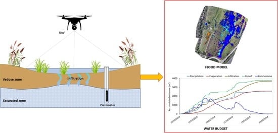
1. Introduction

Coastal wetlands are transitional environments characterised by their complexity, dynamism and large gradients of abiotic variables given their shared features between freshwater and marine ecosystems. Although wetlands only occupy 5–6% of the Earth’s surface [1], their value substantially exceeds their modest share of land-use owing to the many ecosystem services they provide [2]. These enclaves not only underpin great primary production and biodiversity, but also play an important role in nutrient cycling, carbon sequestration, water purification and storage, flood control and local climate regulation, among others. Besides, wetlands provide a range of cultural, recreational and educational resources that contribute to human wellbeing and enrich urban and peri-urban areas [3,4,5].

Once considered insalubrious and unproductive areas, these ecosystems have undergone a sharp decline since the 19th century owing to resource exploitation, eutrophication, land reclamation and fragmentation or drainage with developmental purposes. However, the second half of the 20th century witnessed notable changes in the management policies of these spaces, whose importance started to be recognized internationally. This led to the enactment of longstanding conventions and instruments, such as the Ramsar Convention [6], the Habitats Directive [7], the Convention of Biological Diversity [8] and the European Water Framework [9]. Since then, numerous wetland restoration initiatives have been carried out internationally with promising results [10,11,12]. However, despite these efforts, the global rate of wetland loss has continued to increase in the 20th and early 21st centuries, especially in the case of coastal wetlands, with overall rates 4.2 times faster than those recorded in the long term since 1700 [13]. In this scenario, the creeping hazard of climate change adds up to the disturbances directly induced by human activity. Studies on the impacts of climate change in Mediterranean regions, one of the planet´s hot spot for this phenomenon, consistently point to warmer and drier conditions, substantial reductions in precipitation and freshwater inflows in arid and semiarid areas and to sea level rise [14,15]. In addition, the shift in species distribution is expected to alter the structures of biological communities and the inter and intraspecific interactions between organisms [16,17].

Wetlands are products of their hydrological regime; changes in a wetland´s water table, hydroperiod and flood pulses condition the type of water body and affect many processes, such as groundwater recharge, biogeochemical cycles, heat exchange and gas emissions [18,19]. Hence, the sustainable management of wetlands and protection of their values largely depend on the knowledge of their water budget and its seasonal/multi-year fluctuations. The water budget represents the balance between inflows and outflows within the system, which is controlled by the interactions between different environmental compartments: atmosphere (precipitation, evaporation and evapotranspiration), groundwater (infiltration, discharge), surface water (runoff) and the ocean (tidal/storm flooding), in the case of coastal wetlands. Although many of these hydrological components can be estimated directly using a range of tools, such as precipitation and stream gages, evaporation pans, infiltrometers, automated sensors or the use of environmental tracers, there is still a great deal of uncertainty in the quantification of the water budget owing to the complex and heterogeneous nature of these systems and the inaccuracies of the techniques used to collect data [20]. Moreover, it is crucial to have an accurate picture of the system´s bathymetry as it determines wetland storage and influences the residence time, sediment trapping and flood retention [21]. The available methods for bathymetric mapping of wetlands are diverse in terms of applicability, costs and sophistication, ranging from meter sticks, lasers, total stations, or handheld GPS devices to ground-based LiDAR or satellite imagery. In this regard, the recent development of UAV (Unmanned Aerial Vehicle) photogrammetry and LiDAR (Light Detection and Ranging) techniques is revolutionizing the field of topography, allowing us to produce digital terrain models (DTMs) with very high resolution. Although UAV remote sensing is especially suitable for small scale systems, the accuracy of the topographical products can be greatly influenced by the presence of vegetation, what makes necessary the application of tailored ground-filtering algorithms [22,23].

In recent years, novel approaches based on the combination of remote and in situ observations have been developed to quantify and monitor the interactions between surface water and groundwater systems. For instance, Refs. [24,25] analysed the interactions between wetlands and groundwater and quantified the elements of the water budget by combining airborne LiDAR cartography for the morphometrical definition of the basins, water stage measurements and continuous piezometric records from automatic level loggers. On the other hand, Ref. [26] merged UAV-borne imagery and SfM (Structure from Motion) algorithms with resistivity tomography to assess storage in a Brazilian savanna wetland and to propose a model of wetland–aquifer interaction. In [27], information from LiDAR sensors, photogrammetric surveys and satellite images were integrated with in-situ water level records to investigate the historical variations in water storage and the water budget of an intermittent wetland in Australia.

The objective of this paper is to estimate the elements of the water budget of a small ephemeral coastal wetland and their temporal evolution over a flooding episode, including its interactions with the underlying aquifer through an innovative combination of UAV imagery and in situ observations from a hydrogeological monitoring network. The application of SfM algorithms enabled to define wetland morphology through the generation of a high-resolution DTM, which has been subsequently validated using RGB images of a flood episode. Additionally, the use of automated water level sensors from the control network allowed us to monitor the temporal evolution of wetland stage, the piezometric level and tidal fluctuations on a 10-min basis. This work evidence that the combination of remote sensing with conventional hydrogeological techniques allows us to improve the knowledge on the functioning of complex hydrogeological systems and opens new horizons for the estimation of variables that are difficult to quantify through traditional methodologies.

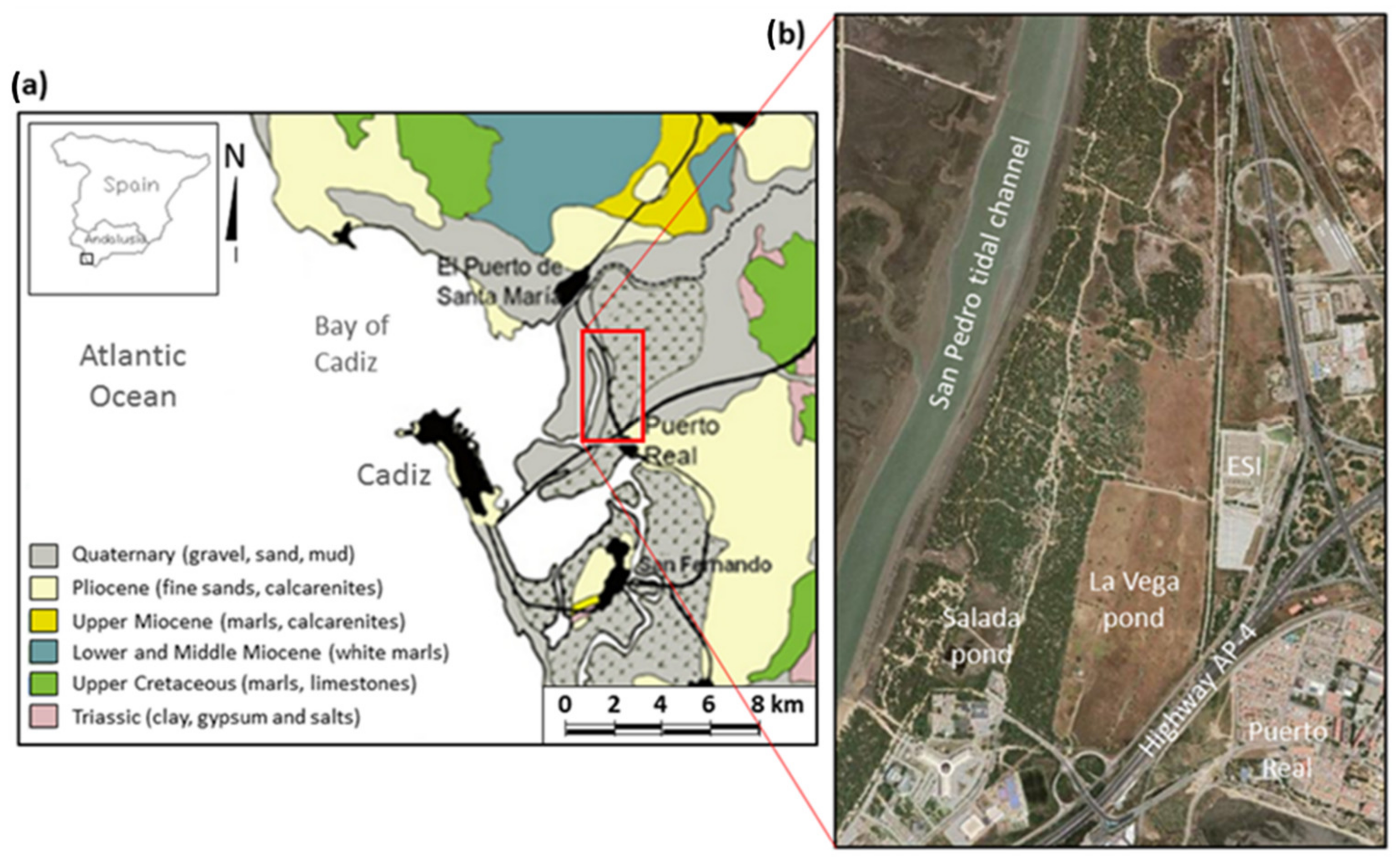
2. Characterization of the Study Area

The study area is located on the SW Atlantic coast of the Iberian Peninsula that shapes the Gulf of Cadiz (Figure 1a). The geological context of this region comprises the eastern end of the Baetic mountain ranges and the south of the Guadalquivir River depression. Its proximity to the margin between the African and Eurasian plates has led to an intense tectonic activity that affects the coastal and seabed physiography and controls the distribution of sedimentary media.

The Bay of Cadiz is located in the SE sector of the Gulf of Cadiz. The bay´s sedimentary environments are controlled by a complex system of barrier islands that limit a wide area of ponds and salt marshes, where a vast tidal flat develops. Tidal deltas, streams and tidal channels abound in this area. Specifically, the study area is located on the left bank of San Pedro tidal channel, in the sector known as the Metropolitan Park of Toruños and Pinar de la Algaida, next to the estuary of the Guadalete River [28] (Figure 1b).

The region displays a very smooth orography (altitude < 4 m above sea level, henceforth m.a.s.l) and its coastal strip is characterized by a semi-diurnal, mesotidal hydrodynamic regime with maximum tidal ranges of 3.7 m, which determines the type and characteristics of the sedimentary deposits.

The climatic context of the study area is Mediterranean with Atlantic influence. The average annual precipitation is around 600 mm and rainfall shows a marked seasonal distribution concentrating mainly at the end of autumn and winter months, with very dry summers [29]. The average annual temperature is 18.2 °C with mild winters (monthly average of 12.8 °C in January) and warm summers (monthly average of 24.5 °C in August), especially when the eastern winds (locally known as Levante) blow. These predominant and persistent winds produce important increases in temperature and reduce air moisture notably.

2.1. Geology

From a geological point of view, the study area is constituted by recent post-orogenic detrital materials of Quaternary age and fine granulometry (fine sand), typical of beach-type environments and dunes with aeolian and fluvial influence. There are also muddy materials typical of marsh environments. Sedimentation during the Holocene is highly controlled by sea level fluctuations, tectonic structure, and late tectonic readjustments of the Baetic Cordillera [30]. Specifically, the geotechnical drilling columns collected in the area show a superficial formation of fine sand, with levels with bioclasts from marine organisms and levels with a silt fraction between 7 and 27%, about 6 m thick. As a whole, this formation behaves like a free aquifer with intergranular porosity and medium–low permeability. The previous formation is located on a level between 5 and 15 m thick, depending on the sector, of dark muddy clays, very plastic and with a soft consistency, formed by sedimentation in low-energy media (marsh). The latter functions as the impermeable base of the aquifer. Beneath these materials appear Pliocene–Pleistocene detrital materials consisting of sands, silty sands, sandstones, and conglomerates (Figure 2).

2.2. Soils

Soils in this area are scarcely developed with poorly differentiated horizons; however, a variety of soil types representative of different edaphic processes and various formation factors can be found locally (Figure 3).

Specifically, a low evolution soil with an AC profile appears under the areas with the greatest accumulations of beach sand and dunes, and also under the thin leaf-litter layer from an old pine forest, with broom, juniper and rockrose shrub among other species. The thin, light-coloured epipedion with a low organic matter content is not diagnostic. The high percentage of sands (82–92%) and its horizons constitute a typical arenosol profile (Figure 3a).

There are also topographically depressed areas partially connected to the sea through the San Pedro tidal channel that lead to the formation of saline lagoons where salt concentrates when disconnected from the tidal channel. On the margins of these water bodies grow halophytic vegetation and salt efflorescence appears during the dry periods. The shallow water table causes temporary hydromorphic features that are permanent at depth. The dominant feature is the presence of salts that rise and concentrate on the surface due to evaporation. These soils present Az, Cgz, Cg, Cr1 and Cr2 horizons and are classified as gleyc Solonchak (Figure 3b).

During rainy winters/springs, a set of temporary freshwater ponds of great singularity have formed since the construction of the highway AP-4, which interrupted the surface drainage. The influence of these ponds enables the accumulation of clay and silt over the sands of the depocenters, which are washed towards deeper areas. The nearby water table favours pseudogleyzation processes, generating a mottled horizon with oxidized and reduced zones and leading to the formation of gleyc Cambisols (Figure 3c). The colonization by meadows during winter favours the accumulations of organic matter in the surface horizon at certain areas and the formation of mollic-type surface horizons, leading to their classification as haplic Phaeozems.

2.3. Environmental Values

The study area belongs to the Cadiz Bay Natural Park, a protected area of 10,500 ha approximately that has been included since 2002 in the RAMSAR List of Wetlands of International Importance. Furthermore, in 2003, this area was designated a Special Protection Area for Birds due to its relevance for the maintenance of habitats and species of interest [31].

Although the study area is located in a highly anthropized environment, surrounded by roads and urban, service and industrial areas, it presents a high environmental singularity due to its variety of environmental units, namely salt marshes, fixed dunes with coastal pine–juniper forest, meadows, and temporary or permanent wetlands with fresh or brackish water with different ranges of salinity. The latter characteristic enables the development of a great variety of aquatic habitats that change over time and favours the ecological community richness.

There are up to six temporary ponds with very different characteristics in terms of chemical quality of water and hydroperiod, despite their proximity. In [32] the authors report electrical conductivities between 870 µS/cm in La Vega pond and 4095 µS/cm in Salada pond. The same authors carried out a detailed species inventory in this small area, some of which are endemic, rare or threatened. They identified up to 118 flora species and a large number of invertebrate species that support large seasonal communities of birds. La Vega pond showed the highest vegetation richness, some of them rare or threatened (Frankenia boissieri, Damasonium alisma subs. bourgaei, D. polyspermum, Armeria gaditana and Polypogon maritimus subsp. subspathaceus). Among invertebrates, it is worth mentioning Branchipus cortesi (Branchiopoda, Anostraca), which is endemic from the Iberian Peninsula, Ceriodaphnia reticulata, Macrothrix hirsuticornis, Macrothrix rosea, Scapholeberis rammneri, Moina brachiata, Moina salina, Ephemeroporus phintonicus, Dunhevedia crassa, Alona azorica, Pleuroxus letournexi and Leydigia acanthocercoides (Branchiopoda, Anomopoda). The concentration of this variety of species, some of them highly specialized and adapted to harsh environmental conditions, with functional diversity and ecophysiological capacities, confers special interest to the study area from the conservation, scientific and educational points of view [33].

These temporary ponds are a good example of how the hydrodynamic regime of an area conditions its ecosystems and therefore the land planning and management. The protection of the ecological values of this area even led to the modification of the construction project of an important building of the University of Cádiz (ESI: Higher School of Engineering) at the beginning of the 21st century, whose initial location was planned on one of these floodable areas. Owing to previous environmental studies and to social pressure from conservation groups, the building site was eventually relocated to neighbouring areas.

3. Materials and Methods

Three sources of information have been used in this work: meteorological data, UAV-borne data and records from a hydrological monitoring network. The study period comprised 72 days (1 March to 12 May 2018) and the analyses were conducted at a daily level. The workflow followed is detailed in Figure 4, along with the information sources and data treatments.

3.1. Estimation of Meteorological Variables

The local precipitation in the wetland area was measured using a network of 5 rain gauges that were controlled on a daily basis during the first 54 days of the study period (03/1/18 to 4/23/18). This enabled the obtention of a daily rainfall series highly representative of the study area. In addition, precipitation data from the closest meteorological station (located 6 km from the wetland, in similar geographic conditions) were used to fix anomalies in the rainfall series and for the rest of the study period. This station, operated by the company APEMSA (Aguas de El Puerto, Empresa Municipal), records precipitation automatically in 15-min intervals, along with other meteorological variables. In this regard, it should be pointed out that a low correlation coefficient (r = 0.62) was found between the mean daily precipitation values from the rain gauges located in the wetland and those from the meteorological station of APEMSA.

For the estimation of the daily evaporation rate, the well-known Penman method [34] was used. Penman´s evaporation equation requires daily data on maximum and minimum daily temperature, maximum and minimum daily relative humidity, solar radiation and mean wind speed at 2 m from the ground. These data were obtained from the aforementioned weather station.

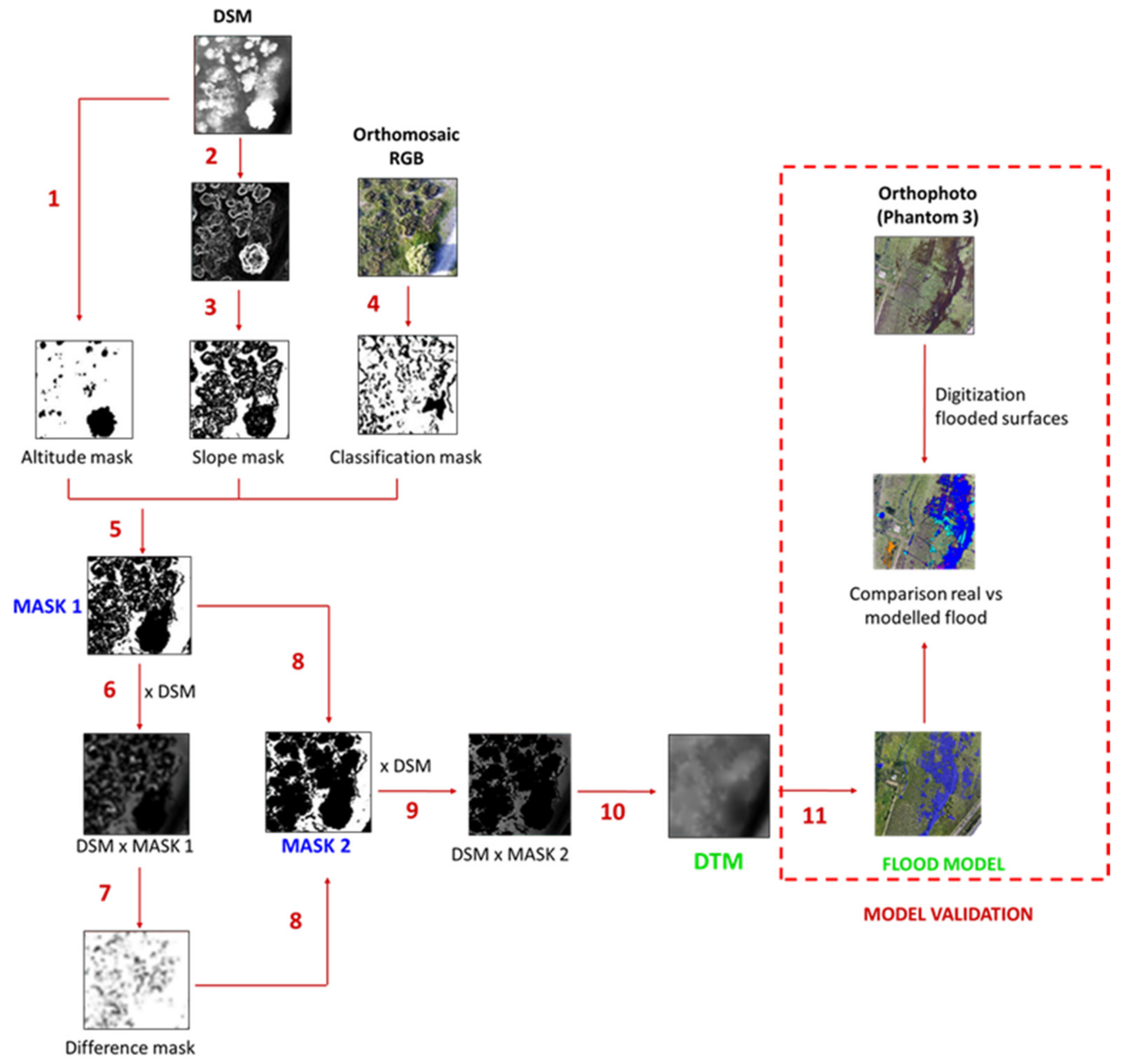
3.2. UAV Photogrammetry

3.2.1. Data Acquisition

Two photogrammetric flights were carried out under contrasting hydrological situations, dry and wet seasons, with different objectives and equipment. The first flight was aimed at defining the morphology of the bottom of the empty pond basin and the subsequent generation of a flood model. The flight was conducted on 17 April of 2017 and data were acquired using an octocopter ATYGES FV-8 (payload of 5 kg) equipped with a Sonny Alpha 7 RGB camera of 24.3 MP and a gimbal stabilisation system. The focal length of the camera is adjustable between 28 and 70 mm and was set at 34 mm and the flight height at 60 m. The flight lasted 13 min and 305 vertical images were captured. To georeference these data, 11 ground control points (GCP) were uniformly distributed throughout the wetland prior to the flight. The three-dimensional coordinates of these GCPs were acquired using a GNSS (Global Navigation Satellite System) model Leica 900 and the reference ground-based station UCA1-13455M002, from the regional GNSS network. The precisions obtained were 0.5 cm in X and Y, and 0.8 cm in Z. For further geometric control and assessment of the accuracy of the 3D model before post-processing, 29 additional checkpoints were selected in the orthomosaic, and their coordinates established using the same GNSS system. These checkpoints ranged in altitude between 1.6 and 2.5 m and consisted of features clearly identifiable both on the ground and in the orthomosaic. Additionally, another 30 checkpoints were selected to assess the accuracy of the model after the post-processing tasks. Both the spatial distribution of GCPs and checkpoints can be consulted in [35].

The second mission was carried out on 20 March 2018, after a period of intense rains that caused the lagoon to partially fill. The objective of this flight was to verify the flood model and readjust the origin of the Z coordinate of the datalogger placed in the pond, in order to make it coincide with the one of the flood models. In this case, data were acquired with a lightweight DJI Phantom 3 Professional quadcopter (payload < 0.5 kg) equipped with a Sony RGB camera with a 12.8 MP EXMOS sensor and a focal length of 3.1 mm, stabilized by a gimbal system. The flight height was 60 m and lasted for 4 min, capturing 91 images. In this case, no control or verification points were used.

3.2.2. Photogrammetric Processing and Accuracy Assessment

The photogrammetric processing of the images obtained in both missions was carried out by applying SfM (Structure from Motion) algorithms, a technique that allows for reconstructing the 3D structures from its projections into a series of images taken from different viewpoints [36]. One of its advantages is that SfM does not require prior knowledge of the camera exposure locations and attitudes. SfM incorporates simultaneous, highly redundant, iterative bundle adjustment procedures based on a database of features automatically extracted from a set of multiple overlapping images [37]. The parameters of the camera and characteristic elements of photographs are solved automatically with very little user interaction [38].

The processing was performed using Pix4D version 3.2 software with the template for 3Dmaps. The Pix4D workflow basically consists of three steps: initial processing, point cloud densification, and DSM (Digital Surface Model) and orthomosaic generation. The user-defined properties which guide the quality, accuracy, and format of the final output are all handled through the processing options dialogue box which must be set up prior to any processing steps.

Table 1. Processing results obtained with Pix4D software.

	First Mission (17 April 2017)	Second Mission (20 March 2018)
System	ATYGES FV-8	Phantom 3
Number of images	305	91
Average GSD (cm)	1.38	3.26
Key points per image (median)	88,241	45,897
Matches per calibrated images (median)	43,077	24,242
Number of GCP	11	0
Number of 2D key points observations for bundle block adjustment	12,709,676	2,143,762
Number of 3D points for bundle block adjustment	4,595,853	797,045
Mean reprojection error (pixels)	0.133	0.179

shows the main characteristics of the processing results.

The cartographic products obtained from the first flight were an RGB orthomosaic and a DSM with spatial resolutions of 1.38 and 6.90 cm, respectively. In the second flight, only one RGB orthomosaic with resolution 3.26 cm was generated.

In the first mission the GCPs were used to transform the image coordinates to an absolute coordinate system (WGS84, UTM29N, EPSG 32629). In the second mission such transformation was not necessary because the orthomosaic was transformed and forced to geometrically match with the orthomosaic from the first mission, which had better geometric quality. This transformation was performed with the software ENVI 4.3, specifically the module “Map-Registration”, applying a 3rd degree polynomial function whose coefficients were adjusted using the control point method. A total of 31 GCPs distributed throughout the image were considered, and the total root mean square error (RMSE) was 1.5 cells.

As for the DSM obtained, the altimetric accuracy was evaluated by comparing the Z value with the Z-coordinate of the checkpoints, obtaining an RMSE_Z of 3.5 cm before post-processing [35] with a slight positive deviation of about 2 cm, which implies a slight underestimation of the DSM values in the vertical axis Z. This positive deviation is similar to the one found by [39].

3.2.3. Post-Processing

As stated in Section 2.3, the study area is partially occupied by shrubs of different species, which hinders the observation of the terrain. To remove the effect of vegetation and transform the DSM into a DTM, a combination of criteria was applied throughout the treatment of the images, which was carried out in a GIS environment (software gvSIG version 2.2). The criteria adopted, fully detailed in [30], are as follow: (1) Cells without significant influence of vegetation keep their Z values unaltered. (2) Cells where the Z value is altered due to the presence of vegetation are cancelled and incorporated into the vegetation mask. (3) The identification and isolation of cells influenced by vegetation is performed by a combination of geometric (elevation and slope thresholds) and spectral criteria, and (4) the final product is obtained by filling the cells corresponding to vegetated areas through a procedure that considers the Z values of the edges around the gaps without modifying the rest of cells. The scheme of operations performed is detailed in Figure 5.

In the first stage, an elevation-filtering mask was applied to eliminate pixels with elevations greater than 2.4 m, which clearly correspond to shrub-type vegetation. Afterwards, the topography was modelled by computing slopes with kernel 7 × 7 (48.3 × 48.3 cm), and slopes above 10° were removed using a second mask. Then, the application of the parallelepiped supervised classification method allowed us to recognize the pixels corresponding to vegetation and shadows, which were subsequently eliminated using a third mask. The three masks were multiplied to combine their effects; this new product is referred as “Mask 1” henceforth. Then, Mask 1 was overlapped to the original DSM and, subsequently, a filtering of minima was applied and a new mask was generated for the removal of cells that exceed a given value; the product of these operations will be referred as “Difference mask”. Then, “Mask 1” was combined with the “Difference mask” to obtain “Mask 2”, a product that includes all the cells identified as vegetation. Mask 2 was multiplied by the original DSM and the final DTM was obtained by filling the cells attributed to vegetation using splines [40].

Once generated, the quality of the DTM at vegetated areas was verified using the three-dimensional coordinates of 30 additional checkpoints measured in situ, as indicated in the previous section. In this case, the RMSE_Z was somewhat higher (7.5 cm) than that obtained for non-vegetated areas.

Afterwards, the DTM´s histogram was used to extract the surface below each water level stage and subsequently to infer the volume stored from the surfaces in a GIS environment. This was performed by applying Equation (1):

$$V_i=\frac{1}{3}h\left(A_i+A_{i-1}+\sqrt{A_i\ast A_{i-1}}\right)$$

(1)

where:

• V_i: volume between elevation i and i−1.
• A_i: number of pixels with elevation ≤ i (obtained from the histogram) multiplied by the area of each cell.
• A_i−1: number of pixels with elevation ≤ i − 1 (obtained from the histogram) multiplied by the area of each cell.
• h: Difference of elevation between i and i − 1.

This enabled us to generate the rating curve of the wetland, which defines the relationship between the water stage and the area/volume stored in the pond.

Finally, the orthomosaic generated in the second flight was used to delineate the flooded area on 20 March of 2018 at 10:00 a.m. and compare it with the prediction of the flood model. Thus, the flooded surface on the orthomosaic was compared with the flooded surfaces of the model for a narrow range of heights around the value recorded by the datalogger placed in the pond in that instant. This allowed us, on the one hand, to identify the extent of coincidences and discrepancies between the model and real, in situ data. On the other hand, this enabled us to readjust by 1.8 cm the origin of the Z coordinate of the datalogger placed in the wetland, in order to improve its matching.

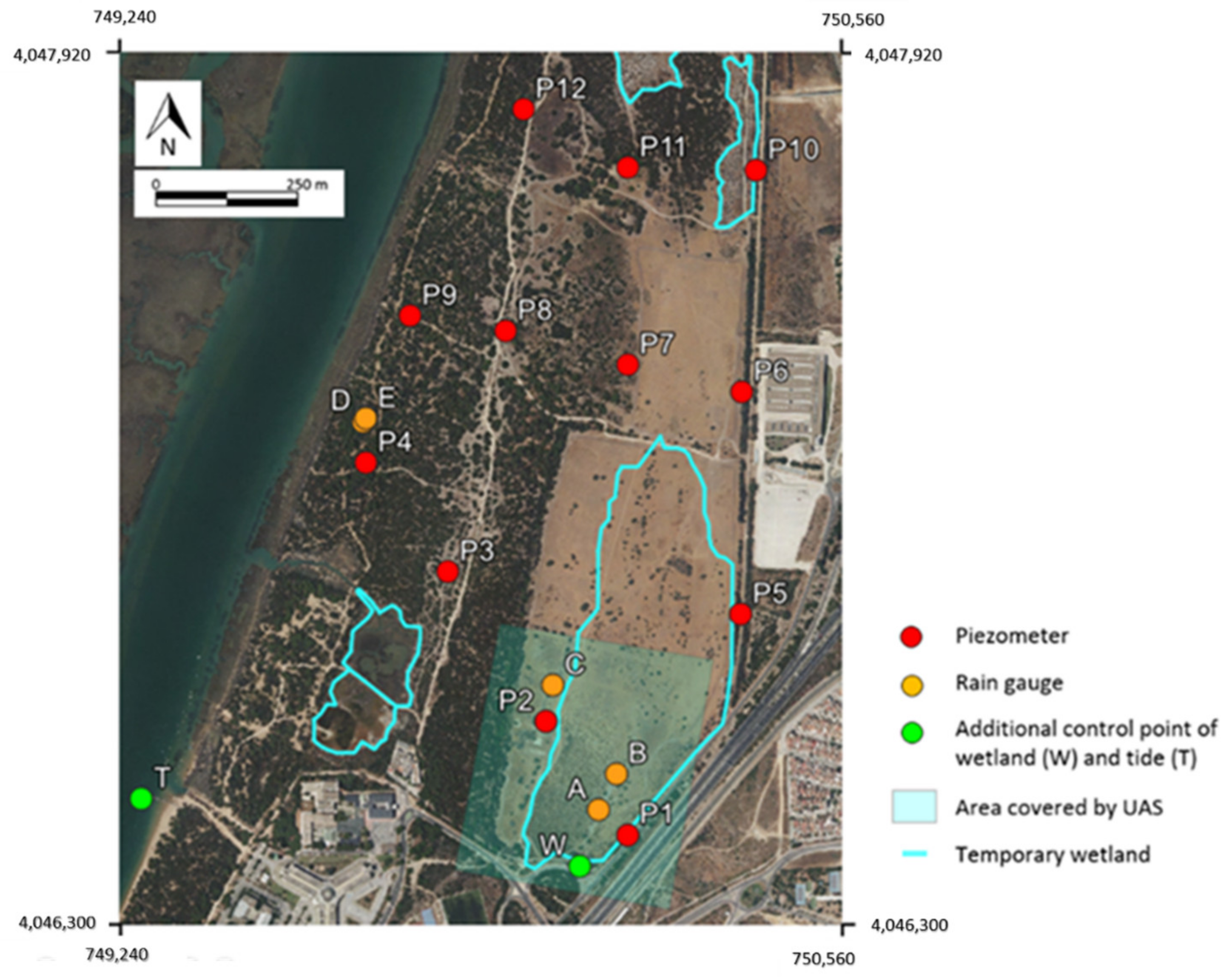
3.3. Hydrological Monitoring Network

A network of piezometers built by the authors [41] in 2015 has been used to collect data from the sandy aquifer underneath the wetland (Figure 6). The network consists of 12 shallow perforations (diameter 75 mm, 3 m deep) that have been adapted as observation piezometers. These piezometers are distributed in an area of 1500 × 750 m and are arranged in 3 transects approximately transversal to the left bank of the San Pedro tidal channel, which constitutes the main discharge zone. The groundwater observation network was completed with a control point of the water stage of La Vega pond and with another point to monitor the tidal fluctuations in the San Pedro tidal channel.

Depending on the season, the hydrological network was equipped with up to 8 dataloggers. This work considers the records obtained between 1 March and 12 May 2018, a particularly rainy period that led to a large accumulation of water in the pond. During this period, data on water stage and piezometric level at P1, P4 and P5 were obtained at 10-min intervals. This allowed the precise identification of the response of the pond and the underlying aquifer to rainfall events. Additionally, previous records (11/28/2015 to 12/26/2015) of tidal fluctuations at the tidal channel and at piezometer P4 were used to identify the influence of tides on the discharge area of the aquifer.

The dataloggers used were of two models: (i) Solinst model Edge 3001 (accuracy 0.05%) and (ii) LevelSCOUT CT2X from Seametrics (accuracy 0.05%). The variables measured were hydrostatic pressure and temperature, although in this work we only refer to the first. The processing stage involved two successive operations: (i) barometric correction of the datalogger records using the readings of an additional continuous pressure measurement device (barologger), and (ii) data calibration through manual measurements of piezometric level depth and water stage in the pond, with respect to previously levelled points.

3.4. Budget Adjustment and Estimation of Pond–Aquifer Transfers

The final data-processing stage consisted of the estimation of the elements of the balance on a daily level. The flooded surface and the stored volume of the pond were calculated using the pond stage, which was measured with a datalogger in the monitoring network, and the rating curve generated from photogrammetry (see Section 3.2.3). Both variables were estimated for the same hour of each day of the study period, concretely for 12:00 pm. The combination of this information with the meteorological variables calculated as described in Section 3.1, enabled us to define the following elements of the balance, expressed in m³: (i) rainfall input owing to direct precipitation on the pond, (ii) output due to direct evaporation from the pond, and (iii) storage variation, as the difference between the volume stored and that of the previous day.

Afterwards, the rainless periods with absence of surface and subsurface runoff were identified. To achieve this, the criteria applied were that precipitation should be zero or less than 1 mm during the 48 h prior to a given date. Under these conditions, it was assumed that the input by surface and subsurface runoff was negligible and therefore it was possible to calculate the only unknown term from the balance equation: infiltration from the pond to the aquifer. This was achieved according to Equation (2):

Inf_i = (P_i · A_i) − DV_i − (Ev_i · A_i)

(2)

where:

• Inf_i: Infiltration volume on day “i” (m³).
• P_i: Precipitation on day “i” (m).
• A_i: Flooded area on day “i” (m²).
• DV_i: Volume stored on day “i” minus the volume stored on day “i − 1” (in m³).
• Ev_i: Evaporation on day “i” (m).

A total of 30 days met this condition and enabled us to establish a statistical model that relates infiltration to other variables, such as the position of the piezometric level, the pond stage or its average depth. This model has also allowed estimating infiltration during rainy periods, so a second element of the balance could be cleared; surface and subsurface runoff. This was performed by applying Equation (3):

Rf_i = DV_i − (P_i · A_i) + Inf_i + (Ev_i · A_i)

(3)

where:

Rf_i: Runoff volume on day “i” (m³).

The remaining variables are as indicated in Equation (2).

The consideration of the accumulated values throughout the study period enabled us to quantify the volumes involved in each element of the water budget.

4. Results and Discussion

4.1. Validation of the Photogrammetry-Derived Flood Model

The second photogrammetric mission, which took place during a flooding event, enabled us to visually identify the limits of the flood (Figure 7b) and compare them with the flood model obtained from the first photogrammetric mission. Despite some limitations associated with vegetation patches and the difficulty of differentiating flooded from saturated soil, the delineated perimeter can be considered the actual flooded area, with a total surface of 23,467 m².

The rating curve derived from photogrammetry evidenced that the water stage of 1.911 m was the level with greatest concordance with the real flooded area (Figure 7a). This enabled us to readjust the datum of the datalogger from the hydrological monitoring network (point W, Figure 6) and unify the reference system of the recording device (datalogger) and the flood model. This readjustment consisted of a correction of 18 mm, which was justified by the uncertainty inherent to datalogger levelling and the altimetric control points used for georeferencing the DTM.

The simulated flooded surface for a stage of 1.911 m was 23,296 m², which differs from the real flooded area by less than 1%. This ensures an excellent quality in the estimates of volumes and surfaces derived from the model, which are necessary to adjust the water budget of the system, as explained in Section 3.4.

It should be noted that, albeit the agreement between surfaces is very high in absolute terms, there are local mismatches by excess and defect that are eventually compensated. These differences, which are displayed in Figure 7c, evidence local errors in the model attributable to the post-processing applied to eliminate the effect of the vegetation in the DTM and to the subsequent height estimation in areas covered by shrub. These procedures led to an increase in the model´s error, as pointed out in Section 3.2.3. Nevertheless, such errors are countervailed and do not produce a significant deviation in the estimation of the variables involved.

4.2. Analysis of the Tidal Influence on the Aquifer

Figure 8 displays the evolution of the tide level in the Río San Pedro channel, along with the evolution of the piezometric level in the piezometer P4, which is located 100 m approximately from the shore. This record corresponds to a 4-week period in 2015 that, despite being prior to this work, is useful to understand the behaviour of the aquifer in the main discharge area.

The mean tide height (marked as a red dotted line) over that 4-week period was 0.475 m higher that the general altimetry datum of the GNSS measurements, which is a relevant aspect for the definition of the average height of aquifer discharge in that sector.

The temporal evolution of the tide shows high-frequency fluctuations that correspond to the semi-diurnal oscillations typical of the region. In addition, a low-frequency fluctuation with a period of about 2 weeks is observed, which is attributable to the succession of spring tides (amplitude up to 3.0 m) and neap tides (amplitude below 1.6 m).

The piezometric level in P4 shows a general downward trend during these 4 weeks, going from 1.10 m to 0.99 m, as it would be expected in a point close to the discharge zone of an aquifer that did not receive recharge over such a period. The tidal influence is evident through two mechanisms:

(i)

Small oscillations of the piezometric level (<2 cm) caused by semi-diurnal tidal cycles. These oscillations display certain delay with respect to the low tide. Such delay varies depending on tide amplitude and the previous history, and may even occur during high tides, as happened on December 2 and 3 of 2015. The low amplitude of these oscillations is justified by the low transmissivity of the aquifer. Such low transmissivity is the result of the thin saturated zone (whose thickness was estimated at about 3.5 m through geotechnical surveys in the study area) and the low permeability of the materials, which was estimated in laboratory at 3.3 m/day for fine sands with silt and clay contents <7.5%. These data are consistent with the results of a low-flow injection test (0.08 l/s) under transient regime carried out by the authors on the piezometer P4, which displayed a transmissivity of 15 m/day.

(ii)

The stabilization of the piezometric levels owing to spring tides, which makes the aforementioned general downward trend to cease. This phenomenon produces a low frequency oscillation (twice a month approximately) with an estimated amplitude of around 3 cm on the piezometric level. This can be explained by the inversion of hydraulic gradients during the part of the tidal cycle when the water stage in the channel is above the piezometric level, forcing a flux of seawater towards the aquifer. These inputs would compensate over several days the aquifer´s discharge towards the tidal channel when the tide level is below the piezometric level. When neap tides occur again, the piezometric level shows a downward trend with certain delay that evidences discharge into the tidal channel. Therefore, there is a discontinuous entry of seawater that constitutes a saline input into the coastal sector of the aquifer when the piezometric levels are significantly below the high spring tides.

At the beginning of the period covered by this study (1 March 2018), the hydrodynamic situation of the aquifer in the sector near the San Pedro tidal channel was similar to that previously described. Initially, P4 presented a piezometric level of 1.06 m. Later, the piezometric level progressively rose and reached 1.68 m on 23 March 2018, reducing the effect of the inversion of hydraulic gradients in the discharge zone and leading to greater discharge towards that sector.

In any case, the tidal influence on the piezometric level in the vicinity of the wetland through these two mechanisms can be considered negligible (less than 1 cm) owing to aquifer´s low transmissivity and the distance from the piezometers to the shoreline, which dampens the effect of tides on groundwater. This can be justified by the fact that the mean value of the piezometric level around the wetland has been averaged from the records of three piezometers (P1, P4 and P5), as will be described in Section 4.3. Whilst piezometer P4 is located about 100 m from the shoreline, P1 and P5 are more than 500 m away, which evidently exerts a damping effect. In this regard, ref [42] reports that a typical damping distance for the tidal fluctuations in an unconfined aquifer is a couple of hundred meters and [43] notes that the damping rates for tidal fluctuations in phreatic aquifers can be 10–20 times higher than in confined aquifers.

4.3. Estimation of Groundwater Recharge from the Pond

Figure 9 displays the temporal distribution of precipitation and its effect on the wetland–aquifer system during the study period. At first, the pond was dry and the piezometric levels were low, around 1 m.a.s.l. (40–50 cm below the pond bottom). During the first 4 days, there were intense rains that added up 101 mm and caused the pond to start flooding. Piezometer P1 (the closest to the pond) experienced a rapid rise of 75 cm in the piezometric level within 4 days, while P4 and P5 (furthest from the pond) showed a slight rise with increases between 10 and 30 cm. These differences are justified by differences in the thickness of the vadose zone.

Rainfall continued until 18 March, reaching 213 mm, which represents 35% of the mean annual rainfall. On 20 March, when the second flight took place, the pond reached its maximum stage, with a maximum depth of 43 cm. The piezometric level in P1 was similar to the one of the pond, while in P4 and P5 the level was lower but kept displaying an upward trend. A few days later, the piezometric levels and the pond stage began to drop. This trend was again interrupted by the rains that occurred between April 7 and 13 and by subsequent episodes of scarcer precipitation. In total, rainfall during the study period added up 315 mm, which accounts for 52.5% of the average annual rainfall in the area, so that spring season was extraordinarily wet.

The selection of three rainless periods (27 March–6 April, 17–21 April and 30 April–11 May) when surface and subsurface runoff had ceased and there was an absence of inflows into the pond, allowed for estimating the daily volume infiltrated and the daily infiltration rates (in mm) by applying Equation (2) (see Section 3.4). The infiltration rate ranged between 3 and 25 mm/day, with a mean value of 11.6 mm/day. The existence of variable infiltration rates is justified by different hydrodynamic situations (Figure 10). Initially, when the piezometric level is below the bottom of the pond, percolation occurs as a vertical flow through an unsaturated medium and is influenced by the depth of the water column in the pond and the vertical hydraulic conductivity of the detrital formation. When the piezometric surface bulges, the hydraulic gradient becomes progressively reduced and water acquires a horizontal, divergent radial flow. As the piezometric level rises and becomes closer to the pond stage, the flow per unit section decreases. This finding is in line with other studies that point out a decline of soil infiltration capacity as the water table rises and the vadose zone shrinks [44,45,46,47].

In order to find an empirical law that describes the variability of the infiltration rate as a function of other variables, a multiple regression analysis was carried out. The infiltration rate was considered the dependent variable. The independent variables considered were the mean piezometric level, pond stage, average water column depth and average thickness of the vadose zone. The analysis evidenced that all these variables are not independent, instead, they are strongly conditioned by the water stage in the pond. Thus, a single variable, pond stage, can explain most of the variability of the infiltration rate.

Figure 11 shows the relationship between the pond stage and other variables. The orange points correspond to the pond stage at the central furrow, which presents a different behaviour, as will be explained later. Figure 11a displays a very high correlation between the water stage and the piezometric level. The rise in the pond stage results in an increase in the flooded surface and, therefore, in an increase in the filtering surface, which leads to a progressive rise in the piezometric level until the saturated zone reaches the bottom of the pond. Subsequently, during the emptying stage, the lowering in the piezometric level enhances the decrease in the level of the pond.

In general, deeper water columns in a water body implies greater hydraulic pressures over their bottom, which favours higher infiltration rates. Figure 11b presents the relationship between the average water column depth and the water stage in the pond. In this case, the relationship between the variables shows an upward, linear trend up to a stage of 1.80 m; however, if the stage exceeds 1.80 m, the trend reverses and the average depth tend to decrease. This can be explained by the morphology of the pond´s basin, whose relief above 1.80 m has extraordinarily gentle slopes that favour the flooding of large areas with a very low thickness of water column.

Figure 11c shows a more complex relationship between the pond stage and the vadose zone thickness underneath. Those points located where the water stage is lower than 1.80 m display an increasing trend in the thickness of the vadose zone as the water stage keeps rising. Conversely, the vadose zone thickness tends to stabilize and to show greater dispersion when the water stage exceeds 1.80 m. This way, the evolution of the vadose zone thickness in a given moment will depend on the preceding hydrological condition of the pond, that is, the water stage. Finally, Figure 11d shows the relationship between the daily infiltration rate and the stage of the pond. Among the independent variables analysed, the water stage showed the highest correlation with the infiltration rate (R² = 0.84). Therefore, these two variables have been the ones used in this work to estimate the infiltration rate from the water stage. It should be noted that the orange points corresponding to the rating curve of the central furrow (depocenter) have been excluded from this adjustment because this zone tends to accumulate larger proportions of silt and clay that reduce the permeability of the material, as was stated in Section 2.2.

The cited empirical law is Equation Y = −80.09X + 155.52, which has an estimation error of ±3.2 mm/day. This equation allows for estimating the infiltration rate when the existence of unknown inflows into the system hinders the calculation of infiltration. Once the infiltration rate is determined for each of the days of the month, it is possible to apply Equation (3) to estimate the inputs by surface and subsurface runoff in such periods.

Once all the elements of the balance were calculated, the evolution of the accumulated volumes of inflows and outflows from La Vega pond could be represented (Figure 12). The total volume of inflows into the pond accounts for 6244 m³, of which 39.8% correspond to direct precipitation over the pond and 60.2% to surface runoff. The outputs were of the same magnitude as the inputs and 41.2% corresponded to direct evaporation from the water surface and the remaining 58.8% to transfers into the aquifer, which is equivalent to an average rate of infiltration of 43 mm during the study period considering the mean area of the wetland.

5. Applicability of the Method, Limitations and Future Research

The application of the proposed methodology requires taking into account several limitations and practical considerations.

The results of this study constitute an initial approximation to the evaluation of the different elements of the water budget of the wetland–aquifer system. In this regard, the precise measurement of precipitation in the vicinity of the wetland is essential for determining the inputs into a system. Precipitation displays great spatial variability, which can lead to notable discrepancies between the daily data recorded “in situ” and the records from the nearest meteorological station available (in this case study, it was located 6 km from the pond). Therefore, the use of precipitation data that does not correspond to the immediate surroundings of the wetland introduces an additional source of error.

Likewise, the estimation of evaporation requires the application of semi-empirical methods (such as Penman, the one used in this work) that require measurements of various meteorological variables that are not always available. In addition, the uncertainty inherent to these methods is usually difficult to establish due to the nature of the variable itself.

Another crucial aspect for the adjustment of the water balance is the quality of the DTM, since the rating curve of the wetland is extracted from this cartographic product. Although the use of SfM photogrammetric techniques has enabled the generation of a high-resolution DTM whose geometric quality has been evaluated through checkpoints, in the areas covered by dense shrub vegetation the altimetric error is greater and constitutes an additional source of error. It is thus advisable to monitor the wetland´s dynamic over several flooding episodes, in order to corroborate the results achieved to date. The proposed methodology and in particular the obtention of orthophotographs under different flooding conditions, allows us to verify the quality of the DTM used for the estimation of flood surfaces and stored volumes. However, the methodology described has several limitations, such as the difficulty of identifying the water surface in the orthophoto in densely vegetated sectors or where the water column depth is very shallow, making it difficult to differentiate between saturated soil from flooded soil. This means that the product obtained, which is considered the “ground truth” flood, is also an approximation.

In this respect, the recent development of small-sized LiDAR sensors compatible with UAVs along with the recent advancements in vegetation filtering algorithms, may represent a significant advance in this field and enable the obtention of more accurate DTMs. For instance, in the Bay of Cádiz (SW Spain) [48] has demonstrated that the use of LiDAR can generate accurate DTMs in salt marsh areas, suggesting that these types of sensors can penetrate dense vegetation to some extent. Nevertheless, as this is not always the case, and these authors suggest merging LiDAR photogrammetry with additional techniques, such as multispectral data, which significantly improves the autoclassification of the bare ground and vegetation surfaces. Currently, the authors are working in this line of research, with the aim of contrasting the results obtained with the photogrammetric techniques.

Another aspect to consider is that the origin of the Z coordinate between the two measurement systems used must match. In other words, the measurements of terrain elevation obtained from UAV-based SfM photogrammetry and the measurements of water surface elevation in the wetland obtained from dataloggers, should have the same exact datum. This work has demonstrated that even a vertical displacement of just 2 cm between the datum of both measurement systems can lead to discrepancies in the flood surface of more than 15%, increasing the error associated to the estimation of volume fluctuations and the components of the balance that depend on the flooded surface (such direct precipitation and evaporation from the pond). Thus, the adjustment of both measurement systems is essential, especially when the wetland basin morphology is extremely flat, such as the study case.

In addition, the influence of tides on the piezometric levels should be analysed in coastal wetlands, especially when continuous piezometric level records are not available, since tidal fluctuations can hinder the identification of the relationships between the variables involved. In this case study, albeit the tidal amplitude can exceed 3 m, its influence on the piezometric level is very limited owing to the hydraulic properties of the aquifer. In this regard, the definition of the terrain morphology with a high-resolution DTM is also crucial to identify potential surface inflows of seawater into the pond during spring tides. In this case, although the spring tides exceed the elevation of the wetland basin, the existence of a high dune ridge between the lagoon and the nearest tidal channel prevents their connection on the surface and enables the maintenance of a freshwater pond of meteoric origin.

Finally, the piezometric control of the aquifer is necessary to establish the hydraulic relationship between the wetland and the hydrogeological system, which is very dynamic and changes over time. Remote sensing techniques has serious limitations for the acquisition of data below the ground surface. Although some advances have been recently made in this field with methodologies devised for determining the piezometric level in shallow aquifers through the observation of large-diameter wells using UAVs [49], it is still essential to integrate remote information with records from hydrogeological monitoring networks to achieve a systematic control of the aquifers over time.

6. Conclusions

The combined use of dataloggers and UAV-borne photogrammetry has enabled us to unravel the functioning of a temporary coastal wetland and its complex interactions with the underlying aquifer and the local tidal regime with very high spatiotemporal resolution. The main conclusions that can be drawn from this case study are as follows:

• The understanding of the hydrogeological and topographical context is critical to define groundwater–surface water interactions and the dynamics of seasonal water bodies. In this regard, the DTM obtained through SfM and ground-filtering treatments provided an accurate representation of the basin morphology with a cell size of 6.9 cm and a RMSEz of 5.9 cm. This product combined with water stage records at 10-min intervals, enabled to calculate pond´s stage and volume stored, as well as estimating the balance between water inputs and outputs over a rainy period of 70 days.
• A detailed hydrological analysis requires in situ precipitation records over the studied system since rainfall episodes display high spatial heterogeneity in narrow time windows. In fact, the correlation between the daily rainfall collected in the pond´s rain gauge network and that from the meteorological station located 6 km from the study area was weak.
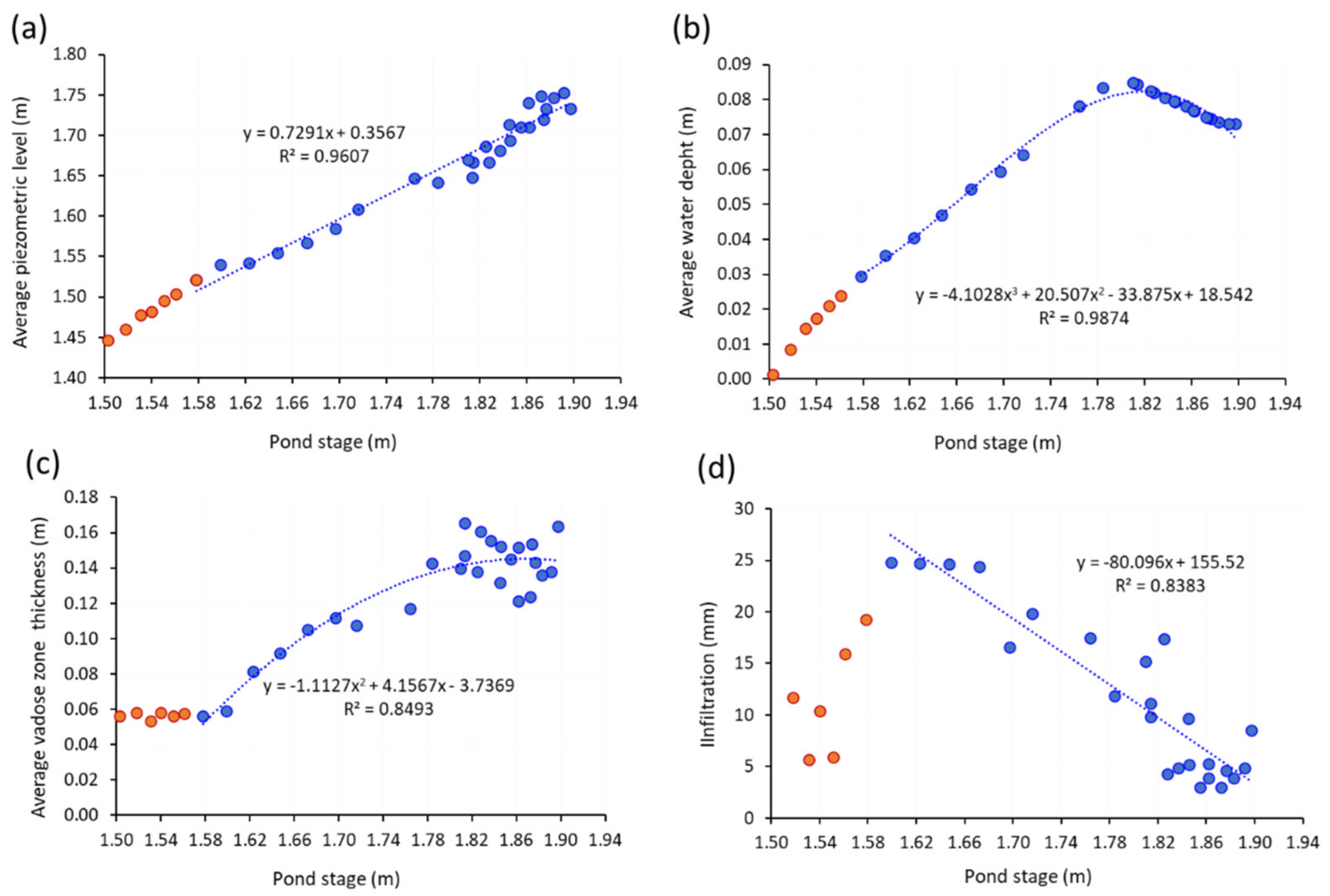
• In this case study, the variable “pond stage” determines the variability of the infiltration rate over time. An empirical law was established between the infiltration rate and the hydrological variable with which the correlation is better: the water stage. This relationship enables us to calculate the infiltration rate under hydrological conditions that do not allow its determination by means of a water balance.
• The application of the proposed methodology has enabled us to quantify the elements of the water budget. During the study period, inflows into the pond accounted for 6200 m³ approximately, of which 40% corresponded to direct precipitation over the pond and 60% to surface runoff. Outputs equalled the inputs, with 41% attributable to direct evaporation from water surface and 59% to transfers into the aquifer.
• The precise definition of the local datum is fundamental to define the marine influence on the aquifer–wetland system, underground flows and flooding during spring tides or storms.
• The proposed methodology constitutes an efficient and economical alternative for elucidating and monitoring the functioning of complex groundwater–surface water systems located in similar hydrological contexts, where high spatial and temporal resolutions are required.

This work evidences that merging remote sensing techniques with conventional hydrogeological approaches allows us to improve knowledge on the functioning of wetland–aquifer systems and opens new horizons for the estimation of hydrological variables that are difficult to quantify through traditional methodologies.

References

- Salimi, S.; Almuktar, S.A.; Scholz, M. Impact of climate change on wetland ecosystems: A critical review of experimental wetlands. J. Environ. Manag. 2021, 286, 112160. [Google Scholar] [CrossRef] [PubMed]
- Janse, J.H.; van Dam, A.A.; Hes, E.M.; de Klein, J.J.; Finlayson, C.M.; Janssen, A.B.; van Wijk, D.; Mooij, W.; Verhoeven, J.T. Towards a global model for wetlands ecosystem services. Curr. Opin. Environ. Sustain. 2018, 36, 11–19. [Google Scholar] [CrossRef]
- Banerjee, O.; Crossman, N.D.; De Groot, R.S. Ecological Processes, Functions and Ecosystem Services: Inextricable Linkages between Wetlands and Agricultural Systems. In Ecosystem Services in Agricultural and Urban Landscapes, 1st ed.; Wratten, S., Sandhu, H., Cullen, R., Costanza, R., Eds.; John Wiley & Sons: Hoboken, NJ, USA, 2013. [Google Scholar] [CrossRef]
- Mitsch, W.J.; Bernal, B.; Hernandez, M.E. Ecosystem services of wetlands. Int. J. Biodivers. Sci. Ecosyst. Serv. Manag. 2015, 11, 1–4. [Google Scholar] [CrossRef]
- Zedler, J.B.; Kercher, S. WETLAND RESOURCES: Status, Trends, Ecosystem Services, and Restorability. Annu. Rev. Environ. Resour. 2005, 30, 39–74. [Google Scholar] [CrossRef]
- Ramsar Convention Secretariat. The Ramsar Convention Manual: A Guide to the Convention on Wetlands (Ramsar, Iran, 1971), 6th ed.; Ramsar Convention Secretariat: Gland, Switzerland, 2013. [Google Scholar]
- Council Directive 92/43/EEC of 21 May 1992 on the Conservation of Natural Habitats and of Wild Fauna and Flora. Available online: https://eur-lex.europa.eu/legal-content/EN/TXT/?uri=celex%3A31992L0043 (accessed on 15 July 2022).
- 93/626/EEC: Council Decision of 25 October 1993 Concerning the Conclusion of the Convention on Biological Diversity. Available online: https://www.eumonitor.eu/9353000/1/j9vvik7m1c3gyxp/vitgbghrkszt (accessed on 15 July 2022).
- Directive 2000/60/EC of the European Parliament and of the Council Establishing a Framework for the Community Action in the Field of Water Policy. Available online: https://eur-lex.europa.eu/legal-content/EN/TXT/?uri=celex%3A32000L0060 (accessed on 15 July 2022).
- Gumiero, B.; Mant, J.; Hein, T.; Elso, J.; Boz, B. Linking the restoration of rivers and riparian zones/wetlands in Europe: Sharing knowledge through case studies. Ecol. Eng. 2013, 56, 36–50. [Google Scholar] [CrossRef]
- Staszak, L.A.; Armitage, A.R. Evaluating Salt Marsh Restoration Success with an Index of Ecosystem Integrity. J. Coast. Res. 2013, 287, 410–418. [Google Scholar] [CrossRef]
- Sullivan, P.L.; Gaiser, E.; Surratt, D.; Rudnick, D.T.; Davis, S.E.; Sklar, F.H. Wetland Ecosystem Response to Hydrologic Restoration and Management: The Everglades and its Urban-Agricultural Boundary (FL, USA). Wetlands 2014, 34, 1–8. [Google Scholar] [CrossRef]
- Davidson, N.C. How much wetland has the world lost? Long-term and recent trends in global wetland area. Mar. Freshw. Res. 2014, 65, 934–941. [Google Scholar] [CrossRef]
- Spencer, T.; Schuerch, M.; Nicholls, R.J.; Hinkel, J.; Lincke, D.; Vafeidis, A.; Reef, R.; McFadden, L.; Brown, S. Global coastal wetland change under sea-level rise and related stresses: The DIVA Wetland Change Model. Glob. Planet. Change 2016, 139, 15–30. [Google Scholar] [CrossRef]
- Manzoni, S.; Maneas, G.; Scaini, A.; Psiloglou, B.E.; Destouni, G.; Lyon, S.W. Understanding coastal wetland conditions and futures by closing their hydrologic balance: The case of the Gialova lagoon, Greece. Hydrol. Earth Syst. Sci. 2020, 24, 3557–3571. [Google Scholar] [CrossRef]
- Borji, M.; Malekian, A.; Salajegheh, A.; Ghadimi, M. Multi-time-scale analysis of hydrological drought forecasting using support vector regression (SVR) and artificial neural networks (ANN). Arab. J. Geosci. 2016, 9, 725. [Google Scholar] [CrossRef]
- Lowe, K.; Castley, J.G.; Hero, J.-M. Resilience to climate change: Complex relationships among wetland hydroperiod, larval amphibians and aquatic predators in temporary wetlands. Mar. Freshw. Res. 2015, 66, 886–899. [Google Scholar] [CrossRef]
- Zhang, L.; Thomas, S.; Mitsch, W.J. Design of real-time and long-term hydrologic and water quality wetland monitoring stations in South Florida, USA. Ecol. Eng. 2017, 108, 446–455. [Google Scholar] [CrossRef]
- Helton, A.M.; Ardón, M.; Bernhardt, E.S. Hydrologic Context Alters Greenhouse Gas Feedbacks of Coastal Wetland Salinization. Ecosystems 2019, 22, 1108–1125. [Google Scholar] [CrossRef]
- Healy, R.W.; Winter, T.C.; LaBaugh, J.W.; Franke, L.O. USGS Circular 1308: Water Budgets: Foundations for Effective Water-Resources and Environmental Management. US Geol. Surv. Circ. 2007, 1308, 90. [Google Scholar]
- Anderson, J.T.; Davis, C.A. Wetland techniques. In Wetland Techniques, 1st ed.; Springer: Dordrecht, The Netherlands, 2013; Volume 3. [Google Scholar] [CrossRef]
- Anders, N.; Valente, J.; Masselink, R.; Keesstra, S. Comparing Filtering Techniques for Removing Vegetation from UAV-Based Photogrammetric Point Clouds. Drones 2019, 3, 61. [Google Scholar] [CrossRef]
- Chen, S.; Johnson, F.; Drummond, C.; Glamore, W. A new method to improve the accuracy of remotely sensed data for wetland water balance estimates. J. Hydrol. Reg. Stud. 2020, 29, 100689. [Google Scholar] [CrossRef]
- Brannen, R.; Spence, C.; Ireson, A. Influence of shallow groundwater-surface water interactions on the hydrological connectivity and water budget of a wetland complex. Hydrol. Process. 2015, 29, 3862–3877. [Google Scholar] [CrossRef]
- Gil-Márquez, J.; Andreo, B.; Mudarra, M. Comparative Analysis of Runoff and Evaporation Assessment Methods to Evaluate Wetland–Groundwater Interaction in Mediterranean Evaporitic-Karst Aquatic Ecosystem. Water 2021, 13, 1482. [Google Scholar] [CrossRef]
- Furlan, L.M.; Rosolen, V.; Salles, J.; Moreira, C.A.; Ferreira, M.E.; Bueno, G.T.; Coelho, C.V.D.S.; Mounier, S. Natural superficial water storage and aquifer recharge assessment in Brazilian savanna wetland using unmanned aerial vehicle and geophysical survey. J. Unmanned Veh. Syst. 2020, 8, 224–244. [Google Scholar] [CrossRef]
- Chen, S.; Johnson, F.; Glamore, W. Integrating Remote Sensing and Numerical Modeling to Quantify the Water Balance of Climate-Induced Intermittent Wetlands. Water Resour. Res. 2021, 57. [Google Scholar] [CrossRef]
- Muñoz Pérez, J.J.; Jofré, J.M.; Pérez-Fortis, M.J.; De la Casa, Á. Procesos de inundabilidad en la zona marismal de Los Toruños (Cádiz). Tecnoambiente Rev. Prof. Tecnol. Equip. Ing. Ambient. 1999, 9, 35–38. [Google Scholar]
- Consejería de Medio Ambiente, Junta de Andalucía. Decreto 79/2004, de 24 de febrero, por el que se aprueban el Plan de Ordenación de los Recursos Naturales y el Plan Rector de Uso y Gestión del Parque Natural Bahía de Cádiz. 2004. Available online: https://www.juntadeandalucia.es/boja/2004/71/2 (accessed on 23 August 2022).
- Gutiérrez-Mas, J.M.; García-López, S. Recent evolution of the river mouth intertidal zone at the Río San Pedro tidal channel (Cádiz Bay, SW Spain): Controlling factors of geomorphologic and depositional changes. Geol. Acta 2015, 13, 123–136. [Google Scholar] [CrossRef]
- Junta de Andalucía. DECRETO 79/2004, de 24 de febrero, por el que se aprueban el Plan de Ordenación de los Recursos Naturales y el Plan Rector de Uso y Gestión del Parque Natural Bahía de Cádiz. 2013. Available online: https://www.juntadeandalucia.es/medioambiente/portal/landing-page-planificacion/-/asset_publisher/Jw7AHImcvbx0/content/porn-y-prug-del-parque-natural-bah-c3-ada-de-c-c3-a1diz-incluye-los-parajes-naturales-isla-del-trocadero-y-marismas-de-sancti-petri-/20151 (accessed on 15 August 2022).
- García de Lomas, J.; García, C.M.Y.; Canca, I. Caracterización y fenología de las lagunas temporales del Pinar de La Algaida (Puerto Real, Cádiz). Rev. Soc. Gaditana Hist. Nat. 2004, 4, 105–124. [Google Scholar]
- Pérez Hurtado, A.; García-Jiménez, C. Estudio de la adecuación y acondicionamiento para instalaciones y actuaciones de investigación y uso público de los terrenos colindantes al Río San Pedro, Puerto Real, Cádiz. Unpublished Report. 2004; 89p. [Google Scholar]
- Penman, H.L. Natural evaporation from open water, bare soil and grass. In Proceedings of the Royal Society of London Series A–Mathematical and Physical Sciences; The Royal Society: London, UK; Volume 193, p. 120.
- García-López, S.; Ruiz-Ortiz, V.; Barbero, L.; Sánchez-Bellón, Á. Contribution of the UAS to the determination of the water budget in a coastal wetland: A case study in the natural park of the Bay of Cádiz (SW Spain). Eur. J. Remote Sens. 2018, 51, 965–977. [Google Scholar] [CrossRef]
- Schönberger, J.L.; Frahm, J.M. Structure from motion revisited. In Proceedings of the IEEE Conference on Computer Vision and Pattern Recognition (CVPR), Las Vegas, NV, USA, 27–30 June 2016; Institute of Electrical and Electronics Engineers (IEEE): New York, NY, USA, 2016. [Google Scholar]
- Snavely, N.; Seitz, S.M.; Szeliski, R. Skeletal graphs for efficient structure from motion. In Proceedings of the IEEE Computer Society Conference on Computer Vision and Pattern Recognition (CVPR 2008), Anchorage, AK, USA, 24–26 June 2008; pp. 1–8. [Google Scholar]
- Madden, M.; Jordan, T.; Bernardes, S.; Cotten, D.; O’Hare, N.; Pasqua, A. Unmanned Aerial Systems and Structure from Motion Revolutionize Wetlands Mapping. In Remote Sensing of Wetlands: Applications and Advances, 1st ed.; CRC Press: Boca Raton, FL, USA, 2015; 28p. [Google Scholar]
- Contreras-De-Villar, F.; García, F.J.; Muñoz-Perez, J.J.; Contreras-De-Villar, A.; Ruiz-Ortiz, V.; Lopez, P.; Garcia-López, S.; Jigena, B. Beach Leveling Using a Remotely Piloted Aircraft System (RPAS): Problems and Solutions. J. Mar. Sci. Eng. 2020, 9, 19. [Google Scholar] [CrossRef]
- Schweikert, D.G. An interpolation curve using spline in tension. J. Math. Phys. 1966, 45, 312–313. [Google Scholar] [CrossRef]
- García-López, S.; Ruiz-Ortiz, V.; Sánchez-Bellón, A.; Muñoz-Arroyo, G.; Luján, M. Creación de un laboratorio natural de Hidrología en el Parque Metropolitano de Los Toruños y su Aplicación Docente; III Jornadas de Innovación Docente Universitaria, Universidad de Cádiz: Puerto Real, Spain, 2017; pp. 445–448. ISBN 978-84-697-4354-6. [Google Scholar]
- Nielsen, P. Tidal dynamics of the water table in beaches. Water Resour. Res. 1990, 26, 2127–2134. [Google Scholar] [CrossRef]
- Li, L.; Jeng, D.S.; Barry, D.A. Tidal fluctuations in a leaky confined aquifer: Localised effects of an overlying phreatic aquifer. J. Hydrol. 2002, 265, 283–287. [Google Scholar] [CrossRef]
- Ramberg, L.; Wolski, P.; Krah, M. Water balance and infiltration in a seasonal floodplain in the Okaying Delta Botswana. Wetlands 2006, 26, 677–690. [Google Scholar] [CrossRef]
- Mangangka, I.M. The Decline of Soil Infiltration Capacity Due To High Elevation Groundwater. Civ. Eng. Dimens. 2008, 10, 35–39. [Google Scholar]
- Brunner, P.; Simmons, C.T.; Cook, P.G. Spatial and temporal aspects of the transition from connection to disconnection between rivers, lakes and groundwater. J. Hydrol. 2009, 376, 159–169. [Google Scholar] [CrossRef]
- Shadab, M.A.; Hesse, M.A. Analysis of Gravity-Driven Infiltration With the Development of a Saturated Region. Water Resour. Res. 2022, 58, 27. [Google Scholar] [CrossRef]
- Curcio, A.C.; Peralta, G.; Aranda, M.; Barbero, L. Evaluating the Performance of High Spatial Resolution UAV-Photogrammetry and UAV-LiDAR for Salt Marshes: The Cádiz Bay Study Case. Remote Sens. 2022, 14, 3582. [Google Scholar] [CrossRef]
- García-López, S.; Vélez-Nicolás, M.; Zarandona-Palacio, P.; Curcio, A.; Ruiz-Ortiz, V.; Barbero, L. UAV-borne LiDAR revolutionizing groundwater level mapping. Sci. Total Environ. 2023, 859, 16. [Google Scholar] [CrossRef]